Parton Distributions in Impact Parameter Space

Abstract

Fourier transform of the generalized parton distributions (GPDs) at zero skewness with respect to the transverse momentum transfer gives the distribution of partons in the impact parameter space. We investigate the GPDs as well as the impact parameter dependent parton distributions (ipdpdfs) by expressing them in terms of overlaps of light front wave functions (LFWFs) and present a comparative study using three different model LFWFs.

I Introduction

Deeply virtual Compton scattering (DVCS) $\gamma^{*}(q)+p(P)\rightarrow\gamma(q^{\prime})+p(P^{\prime})$, where the virtuality of the initial photon $Q^{2}=-q^{2}$ is much large compared to the squared momentum transfer $t=-(p-p^{\prime})^{2}$, provides a valuable probe to the structure of the proton near the light cone. At leading twist, QCD factorization holds and DVCS amplitude can be expressed as a convolution in $x$ of the hard $\gamma^{*}q\rightarrow\gamma q$ Compton amplitude with the generalized parton distributions (GPDs) GPD . Here $x$ is the light cone momentum fraction of the active quark. The skewness $\zeta={Q^{2}\over 2P\cdot q}$ measures the longitudinal momentum transfer in the process.

GPDs are richer in content about the hadron structure than ordinary parton distributions (pdfs). On one hand, $x$ moment of the GPDs give hadron form factors measurable in exclusive $ep\rightarrow ep$ scattering, on the other hand in the forward limit, i. e. for zero momentum transfer, they reduce to ordinary pdfs measurable in inclusive processes. Thus they provide a unified picture of the hadron.

GPDs are off-diagonal overlaps of light-front bilocal operators and unlike ordinary pdfs, they do not have an interpretation of probability densities. It has been shown in bur that a Fourier transform (FT) of the GPDs with respect to the transverse momentum transfer $\Delta_{\perp}$ at zero skewness $\zeta$ gives the distribution of partons in the transverse position or impact parameter space. They are called impact parameter dependent parton distributions (ipdpdfs) $q(x,b_{\perp})$. The impact representation of pdfs on the light front was first introduced by Soper soper in the context of the FT of the elastic form factor. $q(x,b_{\perp})$ give simultaneous information on the distribution of quarks as a function of $x$ and the transverse distance $b_{\perp}$ of the parton from the center of the proton in the transverse plane. Ipdpdfs obey certain positivity constraints and thus, it is legitimate to physically interpret them as probability densities. In fact, this interpretation is not limited by relativistic effects in the infinite momentum frame. $q(x,b_{\perp})$ are defined for a hadron state at sharp momentum $P^{+}$ localized in the transverse plane such that the transverse center of momentum is at $R_{\perp}=0$ (one can also work with a wave packet state localized in the transverse position space in order to avoid the state to be normalized to a delta function). When the target is transversely polarized, the distribution of partons in the impact space is no longer axially symmetric and the deformation is described by the FT of the GPD $E(x,0,t)$. This distortion has been shown to be connected with Sivers effect metz ; burk1 . A 3-D picture of the quarks and gluons in the proton has been proposed in ji in terms of reduced Wigner distributions which are related to the FT of the GPDs in the rest frame of the proton. In skew it has been shown that a FT in the skewness $\zeta$ provides a boost invariant longitudinal position space picture of the proton and is analogous to optical diffraction obtained in single slit experiment. Thus, GPDs provide a unique picture of the hadron in transverse and longitudinal position space.

GPDs can be expressed in the light-front gauge as overlaps of the light-front wave functions (LFWFs) of the target hadron. These are off-forward overlaps in general and one requires not only a particle number conserving $n\to n$ overlap similar to forward pdfs but also an $n+1\to n-1$ overlap, when the parton number is decreased by two. When $\zeta$ is zero, the second contribution vanishes. GPDs and the ipdpdfs have been investigated in several phenomenological models, for example in chiral quark model for the pion model1 , in the constituent quark model model2 , in terms of a power law ansatz of the light cone wave function for the pion model3 , in the context of investigating the color transparency phenomena model4 , in the transverse lattice framework for the pion model5 and in the lattice framework lattice .

In this work we present a comparative study of the GPDs as well as the ipdpdfs using using several phenomenological models of hadron LFWFs. In orbit DVCS amplitude at one loop in QED has been computed for a fermion. In effect, one represents a spin ${1/2}$ system as a composite of a spin ${1/2}$ fermion and a spin-$1$ vector boson, with arbitrary masses drell . Similar models have been used in dip ; marc . This one loop model is self consistent since it has the correct correlation of different Fock components of the state as given by the light-front eigenvalue equation. In skew a simulated model for the meson has been derived from the above LFWF, by taking a derivative with respect to (wrt) the bound state mass square $M^{2}$, which appears in the denominator of the wave function, thus improving the behaviour of it near the end points at $x=0,1$. In this model, DVCS amplitude is purely real. A similar power law behaviour has been used in power ; model3 to construct the GPDs for a meson. Differentiating once wrt $M^{2}$ generates a mesonlike $k_{\perp}$ behaviour and differentiating wrt internal fermion mass $m^{2}$ and the arbitrary gauge boson mass $\lambda^{2}$ simulates a protonlike behaviour of the LFWFs. We present results in both these models. Models for LFWFs of hadrons in $3+1$ dimensions displaying confinement at large distances and conformal symmetry at short distances have been obtained using ADS/CFT method. We also present ipdpdfs in this model.

II Generalized parton distributions

The kinematics of DVCS process is given in detail in skew . We work in the frame of overlap . We take skewness $\zeta$ to be zero. Momentum transfer is purely transverse;

$$t=(P-P^{\prime})^{2}=-{\Delta_{\perp}}^{2}.$$ (1)

The generalized parton distributions $H$, $E$ are defined through matrix elements of the bilinear vector currents on the light-cone:

$$\int\frac{dy^{-}}{8\pi}\;e^{ixP^{+}y^{-}/2}\;\langle P^{\prime}|\bar{\psi}(0)\,\gamma^{+}\,\psi(y)\,|P\rangle\Big{|}_{y^{+}=0,y_{\perp}=0}$$ (2)

$$= {1\over 2\bar{P}^{+}}\ {\bar{U}}(P^{\prime})\left[\,H(x,\zeta,t)\ {\gamma^{+}}+E(x,\zeta,t)\ {i\over 2M}\,{\sigma^{+\alpha}}(-\Delta_{\alpha})\right]U(P)\ ,$$

here $\bar{P}={1\over 2}(P^{\prime}+P)$ is the average momentum of the initial and final hadron.

The off-forward matrix elements can be expressed as overlaps of the light front wave functions overlap . For non-zero skewness $\zeta$ there are diagonal parton number conserving contributions in the kinematical region $\zeta<x<1$ and $\zeta-1<x<0$. There are off diagonal parton number changing contributions in the region $0<x<\zeta$. In our case $\zeta=0$ and the only relevant kinematical region is $0<x<1$. These correspond to the target helicity non-flip ($++$) and helicity flip ($+-$) contributions, respectively. If we consider a spin $1/2$ target state consisting of a spin $1$ particle and a spin $1/2$ particle, these contributions can be expressed in terms of the $2$-particle LFWFs overlap ,

$$H_{(2\to 2)}(x,0,t) = \int\frac{{\mathrm{d}}^{2}{\vec{k}}_{\perp}}{16\pi^{3}}\Big{[}\psi^{\uparrow*}_{+\frac{1}{2}+1}(x,{\vec{k}^{\prime}}_{\perp})\psi^{\uparrow}_{+\frac{1}{2}+1}(x,{\vec{k}}_{\perp})+\psi^{\uparrow*}_{+\frac{1}{2}-1}(x,{\vec{k}^{\prime}}_{\perp})\psi^{\uparrow}_{+\frac{1}{2}-1}(x,{\vec{k}}_{\perp})$$ (3)

$$~{}~{}~{}~{}~{}~{}~{}~{}~{}~{}~{}~{}~{}~{}~{}~{}~{}~{}~{}~{}~{}~{}~{}~{}~{}~{}+\psi^{\uparrow\ *}_{-\frac{1}{2}+1}(x,{\vec{k}^{\prime}}_{\perp})\psi^{\uparrow}_{-\frac{1}{2}+1}(x,{\vec{k}}_{\perp})\Big{]},$$

$${(\Delta^{1}-{i}\Delta^{2})\over 2M}E_{(2\to 2)}(x,0,t)$$ (4)

$$= \int\frac{{\mathrm{d}}^{2}{\vec{k}}_{\perp}}{16\pi^{3}}\Big{[}\psi^{\uparrow*}_{+\frac{1}{2}-1}(x,{\vec{k}^{\prime}}_{\perp})\psi^{\downarrow}_{+\frac{1}{2}-1}(x,{\vec{k}}_{\perp})+\psi^{\uparrow*}_{-\frac{1}{2}+1}(x,{\vec{k}^{\prime}}_{\perp})\psi^{\downarrow}_{-\frac{1}{2}+1}(x,{\vec{k}}_{\perp})\Big{]},$$

where

$${\vec{k}^{\prime}}_{\perp}={\vec{k}}^{~{}}_{\perp}-(1-x)\ {\vec{\Delta}}_{\perp}\ .$$ (5)

Here $\psi^{\uparrow*}_{\lambda_{1}\lambda_{2}}(x,{\vec{k}^{\prime}}_{\perp})$ is the lowest (two-particle) Fock component of the hadron LFWF with helicity up and $\lambda_{i}$, $i=1,2$ are the intrinsic helicities of the internal particles.

The impact parameter dependent parton distributions are defined from the GPDs by taking a FT in $\Delta_{\perp}$,

$$q(x,b_{\perp})={1\over(2\pi)^{2}}\int d^{2}\Delta_{\perp}e^{-ib_{\perp}\cdot\Delta_{\perp}}H(x,t),$$

$$e(x,b_{\perp})={1\over(2\pi)^{2}}\int d^{2}\Delta_{\perp}e^{-ib_{\perp}\cdot\Delta_{\perp}}E(x,t),$$ (6)

where $b_{\perp}$ is the impact parameter conjugate to $\Delta_{\perp}$.

III Simulated model calculations

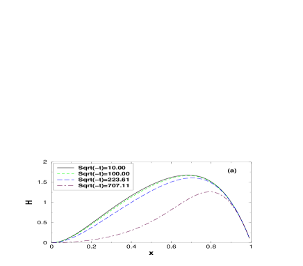
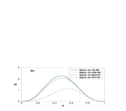
Figure 1: Generalized parton distributions in model $1$; (a) $H(x,0,t)$ and (b) $E(x,0,t)$ as a function of $x$ for fixed values of $\sqrt{-t}$ in units of MeV.

In this section, we calculate the GPDs in simulated models of hadron LFWFs. We start with the two-particle wave function for spin-up electron orbit ; drell ; overlap

$$\left\{\begin{array}[]{l}\psi^{\uparrow}_{+\frac{1}{2}\,+1}(x,{\vec{k}}_{\perp})=-{\sqrt{2}}\ \frac{-k^{1}+{i}k^{2}}{x(1-x)}\,\varphi\ ,\\ \psi^{\uparrow}_{+\frac{1}{2}\,-1}(x,{\vec{k}}_{\perp})=-{\sqrt{2}}\ \frac{k^{1}+{i}k^{2}}{1-x}\,\varphi\ ,\\ \psi^{\uparrow}_{-\frac{1}{2}\,+1}(x,{\vec{k}}_{\perp})=-{\sqrt{2}}\ (M-{m\over x})\,\varphi\ ,\\ \psi^{\uparrow}_{-\frac{1}{2}\,-1}(x,{\vec{k}}_{\perp})=0\ ,\end{array}\right.$$ (7)

$$\varphi(x,{\vec{k}}_{\perp})=\frac{e}{\sqrt{1-x}}\ \frac{1}{M^{2}-{{\vec{k}}_{\perp}^{2}+m^{2}\over x}-{{\vec{k}}_{\perp}^{2}+\lambda^{2}\over 1-x}}\ .$$ (8)

Following the same references, we work in a generalized form of QED by assigning a mass $M$ to the external electrons and a different mass $m$ to the internal electron lines and a mass $\lambda$ to the internal photon lines. The idea behind this is to model the structure of a composite fermion state with mass $M$ by a fermion and a vector ‘diquark’ constituent with respective masses $m$ and $\lambda$. Similarly, the wave function for an electron with negative helicity can also be obtained. In Eq. (8), the bound state mass $M$ appears in the energy denominator. As discussed in skew , a differentiation of the QED LFWFs with respect to $M^{2}$ improves the convergence of the wave functions at the end points: $x=0,1,$ as well as improves the $k^{2}_{\perp}$ behaviour, thus simulating a bound state valence wavefunction. Differentiating once with respect to $M^{2}$ will generate a meson-like behaviour of the LFWF. However, this is not a model for a meson wavefunction since the two constituents have spin half plus spin one. If we differentiate once more we simulate the fall-off at short distances which matches the fall-off wavefunction of a baryon, in the sense that the form factor $F_{1}(Q^{2})$ computed from the Drell-Yan-West formula will fall-off like ${1\over Q^{4}}$. Here we have the analog of a two-parton quark plus spin-one diquark model of a baryon, not three quarks. Overlaps of these wavefunctions in the same way as have been done for the dressed electron wavefunctions will simulate the corresponding GPDs. This is the approach we are following here.

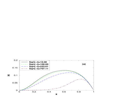
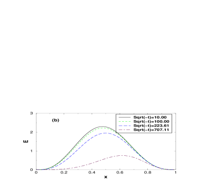
Figure 2: Generalized parton distributions in model $2$; (a) $H(x,0,t)$ and (b) $E(x,0,t)$ as a function of $x$ for fixed values of ${\sqrt{-t}}$ in units of MeV.

We differentiate $\varphi(x,{\vec{k}}_{\perp})$ with respect to the bound state mass $M^{2}$ in order to simulate the LFWFs of a meson-like hadron. In other words, we take

$$\varphi^{\prime}(x,{\vec{k}}_{\perp})=\mid{\partial\varphi(x,{\vec{k}}_{\perp})\over\partial M^{2}}\mid=N\frac{e}{\sqrt{1-x}}\ \frac{1}{\Big{(}M^{2}-{{\vec{k}}_{\perp}^{2}+m^{2}\over x}-{{\vec{k}}_{\perp}^{2}+\lambda^{2}\over 1-x}\Big{)}^{2}}\ ;$$ (9)

where $N$ is the normalization constant. We normalize the $2$- particle LFWF to $1$.

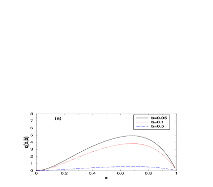
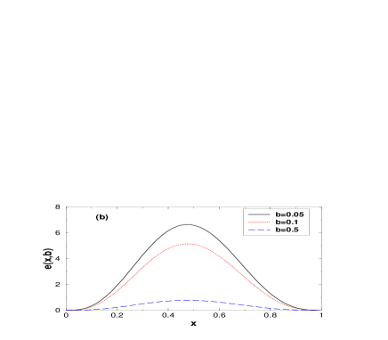
Figure 3: Impact parameter dependent parton distributions in model $1$; (a) $q(x,b_{\perp})$ and (b) $e(x,b_{\perp})$ as a function of $x$ for fixed values of $\mid b_{\perp}\mid$ in units of ${\mathrm{MeV}}^{-1}$

.

The GPD in this model when the target helicity is not flipped (helicity non-flip) becomes (from Eq. (3)):

$$H(x,t) = {e^{2}\over 16\pi^{3}}N^{2}x^{2}(1-x)\Big{[}\Big{(}(1+x^{2})I_{1}+(1+x^{2})I_{2}+\Big{\{}(1+x^{2})P$$ (10)

$$~{}~{}~{}~{}~{}~{}~{}~{}~{}~{}~{}+2(1-x)^{2}(Mx-m)^{2}I_{3}\Big{\}}\Big{)}\Big{]},$$

where

$$I_{1} = \int{d^{2}k_{\perp}\over L_{1}^{2}L_{2}}=\pi\int_{0}^{1}d\beta{\beta\over D^{2}}$$

$$I_{2} = \int{d^{2}k_{\perp}\over L_{1}L_{2}^{2}}=\pi\int_{0}^{1}d\beta{(1-\beta)\over D^{2}}$$

$$I_{3} = \int{d^{2}k_{\perp}\over L_{1}^{2}L_{2}^{2}}=2\pi\int_{0}^{1}d\beta{\beta(1-\beta)\over D^{3}},$$ (11)

here $L_{1}=k_{\perp}^{2}+m^{2}(1-x)+\lambda^{2}x-M^{2}x(1-x)$, $L_{2}=k_{\perp}^{2}-2k_{\perp}\cdot\Delta_{\perp}(1-x)-B$ and

$$D=\beta m^{2}(1-x)-\beta M^{2}x(1-x)+\beta\lambda^{2}x-(1-\beta)B-(1-\beta)^{2}(1-x)^{2}\Delta_{\perp}^{2},$$ (12)

where $B=M^{2}x(1-x)-\Delta_{\perp}^{2}(1-x)^{2}-m^{2}(1-x)-x\lambda^{2}$ and $P=B+M^{2}x(1-x)-m^{2}(1-x)-\lambda^{2}x$.

The helicity flip part as obtained from Eq. 4 is given as:

$$E(x,t)=2MN^{2}{e^{2}\over 8\pi^{3}}x^{3}(1-x)^{3}(Mx-m)I_{3}.$$ (13)

Next, we simulate the LFWF for a proton-like hadron by differentiating eq. (8) first wrt $m^{2}$ and then wrt $\lambda^{2}$. We get,

$$\varphi``(x,{\vec{k}}_{\perp})=\mid{\partial\varphi(x,{\vec{k}}_{\perp})\over\partial m^{2}\partial\lambda^{2}}\mid=\frac{2e}{x(1-x)^{3/2}}\ \frac{{\cal N}}{\Big{(}M^{2}-{{\vec{k}}_{\perp}^{2}+m^{2}\over x}-{{\vec{k}}_{\perp}^{2}+\lambda^{2}\over 1-x}\Big{)}^{3}}\ .$$ (14)

Here ${\cal N}$ is the normalization constant. As before, we normalize the two particle LFWF to 1.

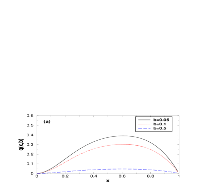
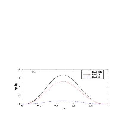
Figure 4: Impact parameter dependent parton distributions in model $2$; (a) $q(x,b_{\perp})$ and (b) $e(x,b_{\perp})$ as a function of $x$ for fixed values of $\mid b_{\perp}\mid$ in units of ${\mathrm{MeV}}^{-1}$.

The helicity non-flip GPD in this model becomes :

$$H(x,t) = {e^{2}\over 4\pi^{3}}{\cal N}^{2}x^{2}(1-x)\Big{[}\Big{(}(1+x^{2})I^{\prime}_{1}+(1+x^{2})I^{\prime}_{2}+\Big{\{}(1+x^{2})P$$ (15)

$$~{}~{}~{}~{}~{}~{}~{}~{}~{}~{}~{}~{}~{}~{}~{}~{}+2(1-x)^{2}(Mx-m)^{2}I^{\prime}_{3}\Big{\}}\Big{)}\Big{]},$$

where

$$I^{\prime}_{1} = \int{d^{2}k_{\perp}\over L_{1}^{3}L_{2}^{2}}=3\pi\int_{0}^{1}d\beta{\beta^{2}(1-\beta)\over D^{4}}$$

$$I^{\prime}_{2} = \int{d^{2}k_{\perp}\over L_{1}^{2}L_{2}^{3}}=3\pi\int_{0}^{1}d\beta{(1-\beta)^{2}\beta\over D^{4}}$$

$$I^{\prime}_{3} = \int{d^{2}k_{\perp}\over L_{1}^{3}L_{2}^{3}}=6\pi\int_{0}^{1}d\beta{\beta^{2}(1-\beta)^{2}\over D^{5}}.$$ (16)

The helicity flip part is given by,

$$E(x,t)=2M{\cal N}^{2}{e^{2}\over 2\pi^{3}}x^{3}(1-x)^{3}(Mx-m)I^{\prime}_{3}.$$ (17)

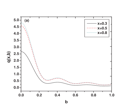
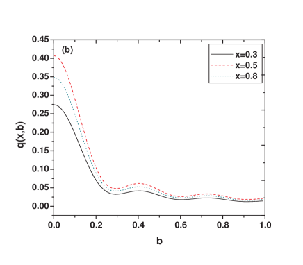
Figure 5: Impact parameter dependent parton distributions $q(x,b_{\perp})$ in (a) model 1 and (b) in model 2 as a function of $\mid b_{\perp}\mid$ in units of ${\mathrm{MeV}}^{-1}$ for fixed values of $x$.

Here we refer to the first model LFWF as model 1 and the second as model 2. In both cases, we take $M=150$  MeV, $m=\lambda=300$  MeV skew . In fig. 1 (a) we have plotted the helicity non flip GPD $H(x,0,t)$ as a function of $x$ for fixed values of $t$. An interesting aspect of these models is that in both of them one can generate a helicity flip contribution $E(x,0,t)$, although the $k_{\perp}$ behaviour of model 1 is similar to a meson. This is because, we have simulated this $k_{\perp}$ behaviour by using a two-particle composite state, where one of the constituents has spin ${1/2}$ and the other has spin $1$. We have plotted the helicity flip GPD $E(x,0,t)$ in model 1 in fig. 1 (b). In figs 2 (a) and (b) respectively, we have shown $H(x,0,t)$ and $E(x,0,t)$ for model 2. From the figs, one can see that the qualitative behaviour of the GPDs in both models are similar. The GPD $H(x,0,t)$ increases with $x$, reaches a maximum and then falls to zero at $x\to 1$ independent of the momentum transfer $t$. As $x$ is the momentum fraction of the active quark and at $x=1$ the active quark carries all the momentum, contributions from the other partons are expected to be zero in this limit and $H(x,0,t)$ is expected to become $t$ independent. The peak of $H$ occurs at higher values of $x$, and it shifts towards even higher values of $x$ as $\mid t\mid$ increases, which means that the active quark is more likely to have a larger momentum fraction. In fact, here we are considering only the leading Fock space component of the target hadron state. Higher Fock space components are more likely to contribute in the small $x$ region. However, the magnitude of the peak decreases for high $\mid t\mid$, which is expected as the form factor decreases with $\mid t\mid$ for high $t$. In model $2$, the peak shifts to larger $x$ faster with an increase of $\mid t\mid$. The GPD $E(x,0,t)$ is associated with the amplitude when the nucleon helicity flips and quark helicity does not flip. This is known to be related to the quark orbital angular momentum. The functional dependence of $E(x,0,t)$ is different from $H(x,0,t)$ in both models. The peak is at $x=0.5$ for smaller values of $\mid t\mid$ but shifts to larger values of $x$ as $\mid t\mid$ increases. It is zero at both $x=0,1$, same as $H(x,0,t)$. Like $H(x,0,t)$, it also becomes independent of $\mid t\mid$ as $x\to 1$. $E(x,0,t)$ decreases as $\mid t\mid$ increases, basically as the first moment of $E(x,0,t)$ gives the form factor $F_{2}(t)$, which decreases for large $\mid t\mid$.

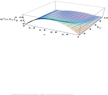
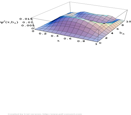
Figure 6: Impact parameter dependent parton distribution in the holographic model.  LHS is for the ground state $L=0,k=1$ and RHS is for the first exited state $L=1,k=1$. $\Lambda_{QCD}=0.32$  GeV and $b_{\perp}$ is given in ${\mathrm{GeV}}^{-1}$.

Taking a Fourier transform (FT) of the GPDs with respect to the transverse momentum transfer $\Delta_{\perp}^{2}$, one gets the ipdpdfs. In figs 3 and 4, we have plotted the ipdpdfs $q(x,b_{\perp})$ and $e(x,b_{\perp})$ defined as in eq. (6) for models 1 and 2 respectively. The ipdpdfs show the same qualitative behaviour in both models, which is expected as the GPDs themselves behave in a similar manner. In other words, qualitatively, parton distributions in the impact parameter space are not that sensitive to the large $k_{\perp}$ behaviour of the LFWFs. The peak is shifted to larger $x$ in model 1. $q(x,b_{\perp})$ goes to zero at $x=0$ and $x=1$. In fact, in the limit $x\to 1$ the active quark with momentum fraction $x$ is very close to the transverse center of momentum, and the transverse width of the ipdpdf vanishes bur . The peak in $x$ decreases as $b_{\perp}$ increases, thus the transverse profile in $b_{\perp}$ is peaked at $\mid b_{\perp}\mid=0$ and falls away further from it. The ipdpdf with the nucleon helicity flip, $e(x,b_{\perp})$ is especially interesting, as for a transversely polarized target, it measures the distortion of the parton distribution in the transverse plane. In addition, the second moment of $e(x,b_{\perp})$ gives how the distribution of momentum of quarks of a particular flavour in the transverse plane changes when the nucleon is not polarized longitudinally. This receives contribution from quarks with nonzero orbital angular momentum and is shown to be connected with Sivers effect. $e(x,b_{\perp})$ is peaked at $x=0.5$ in both models and the height of the peak decreases as $\mid b_{\perp}\mid$ increases. In Fig. 5, we have shown in ipdpdfs $q(x,b_{\perp})$ in both models as a function of $\mid b_{\perp}\mid$ for fixed values of $x$. It is interesting to see that in both models, there is a primary peak at $\mid b_{\perp}\mid=0$ and then there are several secondary peaks. Positions of these secondary maxima are independent of $x$. It is to be noted that in model 2, the curve for $x=0.5$ lies above the one for $x=0.8$, whereas in model 1, the situation is opposite. This is because in model 1, the peak is shifted towards higher values of x than in model 2 (see figs 3 and 4).

In tera , it has been shown that the string amplitude $\Phi(z)$ defined on the fifth dimension in $ADS_{5}$ space can be mapped to the light-front wave functions of hadrons in physical spacetime. The holographic variable $z$ corresponds to the impact variable $\xi$ where $\xi^{2}=x(1-x)b_{\perp}^{2}$, $b_{\perp}$ being the impact parameter. The effective $4$-dimensional Schroedinger equation for the bound states of massless quarks and gluons exactly reproduce the ADS/CFT results and gives a realistic description of the light quark meson and baryon spectrum. The normalized two particle LFWF for the bound state is given by,

$$\Psi_{L,k}(x,b_{\perp})=B_{L,k}\sqrt{x(1-x)}J_{L}(\xi\beta_{L,k}\Lambda_{QCD});$$ (18)

where $B_{L,k}=\Lambda_{QCD}\big{[}(-1)^{L}\pi J_{1+L}(\beta_{L,k})J_{1-L}(\beta_{L,k})\big{]}^{-1/2}$, $\beta_{L,k}$ is the $k$-th zero of Bessel function $J_{L}$ and $\Lambda_{QCD}=0.32$  GeV. For ground state $L=0,k=1$ and we have

$$\Psi_{0,1}(x,b_{\perp})=\Lambda_{QCD}\sqrt{x(1-x)}{J_{0}(\xi\beta_{0,1}\Lambda_{QCD})\over\sqrt{\pi}J_{1}(\beta_{0,1})}.$$ (19)

In fig. 6 we have plotted the ipdpdf for the ground state as well as the first exited state as functions of $x$ and $\mid b_{\perp}\mid$. One has to note that in this model $b_{\perp}$ cannot be very large as $z\leq{1\over\Lambda_{QCD}}$. The primary peak of the ipdpdfs occur for the ground state ($L=0,k=1$) at $\mid b_{\perp}\mid=0$. In the first exited state ($L=1,k=1$) it is shifted away from $\mid b_{\perp}\mid=0$. In both cases, there is a secondary peak at a higher value of $\mid b_{\perp}\mid$ for certain $x$ values. Similar secondary peaks have been observed for the other two models considered, as we already noted.

IV Summary and Conclusion

We have investigated GPDs as well as impact parameter dependent parton distributions at $\zeta=0$ in three different phenomenological models of hadron LFWF. We simulated models for meson-like and proton-like hadrons respectively, starting from the two-particle LFWF of a dressed electron in a generalized form of QED, and differentiating the denominator wrt the squared masses. This improves the behaviour at the end points $x=0,1$ as well as changes the $k_{\perp}$ behaviour. We found that the GPDs and the ipdpdfs are not that sensitive to the $k_{\perp}$ behaviour of the LFWFs. The peak of the ipdpdfs in $x$ for fixed $b_{\perp}$ is shifted towards higher $x$ in the simulated model for a meson-like hadron. We have also investigated the ipdpdfs in the recently proposed QCD holographic model, and shown the behaviour over a larger $b_{\perp}$ range. In all three models, ipdpdfs show several secondary peaks in $b_{\perp}$ besides the primary one.

V acknowledgements

AM would like to thank DST (Fasttrack Scheme), Government of India for financial support.

References

- (1) For reviews on generalized parton distributions, and DVCS, see M. Diehl, Phys. Rept, 388, 41 (2003); X. Ji, J. Phys. G 24, 1181 (1998); A. V. Radyushkin, hep-ph/0101225, published in ”At the Frontier of Particle Physics/Handbook of QCD”, ed. M. Shifman (World Scientific, Singapore, 2001); K. Goeke, M. V. Polyakov, M. Vanderhaeghen, Prog. Part. Nucl. Phys. 47, 401 (2001).
- (2) M. Burkardt, Int. Jour. Mod. Phys. A 18, 173 (2003); M. Burkardt, Phys. Rev. D 62, 071503 (2000), Erratum- ibid, D 66, 119903 (2002); J. P. Ralston and B. Pire, Phys. Rev. D 66, 111501 (2002).
- (3) D. E. Soper, Phys. Rev. D 15, 1141 (1977).
- (4) S. Meissner, A. Metz and K. Goeke, hep-ph/0703176.
- (5) M. Burkardt, Phys. Rev. D 66, 114005 (2002).
- (6) X. Ji, Phys. Rev. Lett. 91, 062001 (2003); A. V. Belitsky, X. Ji and F. Yuan, Phys. Rev. D 69, 074014 (2004).
- (7) S. J. Brodsky, D. Chakrabarti, A. Harindranath, A. Mukherjee, J. P. Vary, Phys. Lett. B 641, 440 (2006); Phys. Rev. D 75, 0143003 (2007).
- (8) W. Bronioski, E. R. Arriola, Phys. Lett. B 574, 57 (2003).
- (9) S. Scopetta, V. Vento, Phys. Rev. D 69, 094004 (2004).
- (10) A. Mukherjee, I. V. Musatov, H. C. Pauli and A. V. Radyushkin, Phys. Rev D 67, 073014 (2003).
- (11) S. Liuti, S. K. Taneja, Phys. Rev. D 70, 074019 (2004).
- (12) S. Dalley, Phys. Lett. B 570, 191 (2003).
- (13) LHPC and SESAM collaboration, Phys. Rev. Lett. 93, 112001 (2004).
- (14) S. J. Brodsky, D. S. Hwang, B-Q. Ma, I Schmidt, Nucl. Phys. B 593, 311 (2001).
- (15) S. J. Brodsky and S. D. Drell, Phys. Rev. D 22, 2236 (1980).
- (16) D. Chakrabarti and A. Mukherjee, Phys. Rev. D 71, 014038 (2005), Phys. Rev. D 72, 034013 (2005).
- (17) A. Mukherjee and M. Vanderhaeghen, Phys. Rev. D 67, 085020 (2003), Phys. Lett. B 542, 245 (2002).
- (18) S. J. Brodsky and F. J. Llanes-Estrada, Eur. Phys. J. C 46, 751 (2006).
- (19) S. J. Brodsky, M. Diehl, D. S. Hwang, Nucl. Phys. 596, 99 (2001).
- (20) S. J. Brodsky and G. F. de Teramond, Phys. Rev. Lett. 96, 201601 (2006).