On Dimer Models and Closed String Theories

1 Introduction

The striking connection between dimer models of statistical mechanics (for reviews, see [1],[2]) and D-brane gauge theories has been the subject of much interest in the last couple of years. The connection, first proposed in [3] was subsequently studied in great details, and it is by now clear that at least for the case of toric singularities, dimer models provide the most robust computational tool for D-brane gauge theories probing the same [4],[5]. This is important especially in the light of the recent extension of Maldacena’s AdS/CFT correspondence to $AdS_{5}\times X^{5}$ spaces, where $X^{5}$ is a Sasaki-Einstein manifold. Although it seems natural that dimer models arise in the connection between quiver gauge theories living on D-brane probes, it has a more direct connection to string theory, which was elucidated, via mirror symmetry, in the beautiful work of [6].

Broadly speaking, the dimer model of a given toric singularity, whose physical interpretation is a collection of NS5 and D5 branes, is obtained by constructing the dual graph of the quiver gauge theory living on the world volume of the D-branes probing the singularity. Given such a dimer model, one can compute certain graph theoretical quantities, which can be shown to relate to the geometry of the singularity being probed by D-branes. The quiver gauge theory of a toric singularity being a purely open string construction, it may seem that computations from dimer models relate solely to open string quantities. However, the geometry of toric orbifolds has an equivalent description in closed string theory, and it is tempting to ask whether one can relate these graph theory quantities to closed strings.

Indeed, it has been shown that there is a correspondence between dimer models and the gauged linear sigma model [7] (called GLSM in the sequel). The dimer-GLSM correspondence was proposed in [4] and proved in [8]. Simply stated, this correspondence states that there is a one to one relationship between the perfect matchings in the dimer model corresponding to the gauge theory probed by a D-brane transverse to a given toric singularity, and the fields in the GLSM that describes the (resolution of the) singularity. Given the fact that there exists purely closed string descriptions of these singularities which also naturally relate to the GLSM, it is probably not surprising that there is indeed a connection between dimer models and closed strings, and the purpose of this paper would be to explore and specify such a connection, and in some sense this is complementary to the results of [8].

A crucial aspect of the results of [3] (and the subsequent papers that developed these ideas more fully) is the fact that the combinatorics of dimer models predict the “multiplicities” of the GLSM fields that arise in the description of gauge theories living on D-branes probing toric singularities. These multiplicites have no obvious analogue in the closed string picture of the resolution of these singularities. However, as we will show in the sequel, perfect matchings of dimer models (explained in the next section) for toric singularities can be shown to specify the twisted sector R-charges of the closed string CFT states that describes the resolution of the singularity. These charges, which specify the GLSM that describes the singularity therefore provide a correspondence between dimers and GLSMs, via closed strings.

Further, we also propose a different method for the counting of perfect matchings corresponding to a given dimer model, which is different from the ones used in [3],[4]. Our method of counting directly uses the R charges of the twisted sectors of closed string theories living on orbifolds, and in a sense gives a direct interpretation of the perfect matchings as GLSM fields. The advantage of this construction is twofold. Apart from providing a new perspective on dimers, it also makes the computation of perfect matchings (and hence multiplicities of GLSM fields) simpler, and puts it in a broader framework.

The paper is organised as follows. In the next section, we briefly review the relevant results on the physics of dimer models, that will set the notations and conventions used in the rest of the paper. In section 3, we examine the dimer model and specify its connection to closed string theories for the known $\mathbb{C}^{2}$ orbifold singularities. Sections 4 deals with singularities corresponding to orbifolds of $\mathbb{C}^{3}$. Finally, we end the paper in section 5, with some comments on generic (non-supersymmetric) orbifolds and their connections with graph theory.

2 Dimer Models and D-brane Gauge Theories on Orbifolds

In this section, we review various known results on dimer models and its relationship with D-brane gauge theories on orbifold singularities. This will also serve to set the notations and conventions used in the rest of the paper.

2.1 D-brane Gauge Theories on Orbifolds

To begin with, we briefly review the construction of quiver gauge theories on D-branes probing orbifold singularities. Since the issue has been studied in great details over the past few years, we will be brief here, and provide a schematic overview of the topic.

The toric data corresponding to a certain quotient singularity can be described in terms of the $U(1)^{N}$ gauge theory of D-branes probing the singularity. The gauge theory is constructed by the prescription due to Douglas and Moore [9]. While the pioneering work of [9],[10] was concerned with D-branes probing (arbitrary) ALE spaces, various results have emerged over the years that have generalised and extended these results to generic toric varieties (for a nice review on the subject and further references, see [11]). Two paradigms have emerged since then regarding the construction of D-brane gauge theories on toric varieties : the forward and the inverse algorithms, which have been studied and refined over the years and culminated in the fast forward and the fast inverse algorithms, using dimer models. Let us start with a brief description of the forward algorithm.

The forward algorithm deals with computation of the moduli space of a given quiver gauge theory (and a superpotential). Consider, eg. the low energy limit of a probe D-brane gauge theory on an orbifold singularity. The action of the discrete orbifolding group on the coordinates and the Chan Paton factors determine the degrees of freedom that survive the orbifolding action, and the quiver diagram encodes all the information about the charges of the unprojected fields. We will be mostly concerned with abelian orbifolds, and in these cases, the $U(1)^{N}$ charges (where $N$ denotes the number of gauge groups modulo an overall $U(1)$ denoting the centre of mass motion of the D-branes) is written as a matrix, $\Delta$.

Now, the F-term (superpotential) equations of the theory, which are not all independent, are solved in terms of the minimal number of independent fields. The solution is expressed in terms of a matrix $K$, such that the original fields in the quiver (denoted by $X_{i}$) are expressed in terms of the independent fields $v_{j}$ as $X_{i}=\prod_{j}v_{j}^{K_{ij}}$. The $K_{ij}$ might have negative entries, and in order to avoid possible singularities which might arise due to this, one introduces a new set of fields $p_{a}$, that are dual to the $v_{i}$s, by computing the dual matrix, $T$, of $K_{ij}$, with $T$ being such that $K.T\geq 0$ for all the entries. In terms of these fields, the original $X_{i}$ are solved as $X_{i}=\prod_{a}p_{a}^{K.T}$. The number of fields $p_{a}$ is not determined apriori, and this leads to multiplicities in the dual description. Typically, the number of $p_{a}$s is more than the number of $X_{i}$s, and for this reason, we need to introduce a certain number of $C^{*}$ actions in order to eliminate redundancies. The charges of the $p_{a}$s under the new set of $C^{*}$ actions are determined using gauge invariance conditions. Further, one can determine the charges of the $p_{a}$s under the original gauge group, using the matrix $\Delta$. These two sets of charges, when concatenated, gives rise to a charge matrix whose kernel gives the geometric data for the resolution of the singularity being probed by the D-branes (note that for $N$ D-branes probing the singularity, we get $N$ copies of the probed geometry). This procedure, first pioneered in [12] gives us a generic method of obtaining the geometric data corresponding to the gauge theory living on a D-brane probing an orbifold singularity.

The reverse procedure, i.e construction of the gauge theory data from the geometric data of the singularity being probed, is what is known as the inverse algorithm, first proposed in [14]. The universal method of obtaining the gauge theory data from the geometric one proceeds via partial resolution of abelian threefold singularities. The given singularity is first embedded into a generic singularity of the form $\mathbb{C}^{3}/\mathbb{Z}_{n}\times\mathbb{Z}_{m}$ (with $n$ and $m$ assumed to be of the minimal values) and by partial resolution of the latter, which leads to the singularity in question, one is able to construct the corresponding gauge theory. From the discussion of the previous paragraph, it is obvious that there are various redundancies involved in the process, and the resulting theory is non-unique. However, these flow to the same universality class in the infrared, and this has been called toric duality and has been shown to be equivalent to Seiberg duality.

The forward and inverse algorithms mentioned in the last two paragraphs have been refined into the fast forward and the fast inverse algorithm by Hanany and his collaborators via the striking connection between gauge theories living on D-brane probes and certain graph theoretical models, known as dimers. The connection arises from the observation that the multiplicities of the GLSM fields that we have mentioned can be determined from a graph that is in some sense dual to the quiver diagram of the gauge theory. The main result of the exercise is that the information about the quiver gauge theory living on D-branes probing a toric singularity is encoded in certain dual graphs. This surprising connection has since been exploited to study various issues relating to gauge theories, via dimer models. Before we elaborate on this, let us briefly recapitulate the essential features of dimer models.

2.2 Dimer Models and Orbifolds

In this subsection we will summarise a few basic features of dimer models. Broadly, dimer models refer to the statistical mechanics of bipartite graphs, i.e graphs which have the property that each vertex can be colored black or white, such that no two vertices of the same color are adjacent. Given such a graph, a perfect matching denotes a subset of edges, (called dimers), such that each vertex is the endpoint of precisely one edge. There can be various possible perfect matchings corresponding to a given bipartite graph, and the statistical mechanics of random perfect matchings have been the subject of much interest.

In [3], a connection between the combinatorics of dimer models and D-brane gauge theories was proposed. Essentially, the connection arises when one considers the “Kasteleyn matrix” for a given brane tiling obtained by dualising the (periodic) quiver diagram of the gauge theory. The determinant of this matrix, called the charactaristic polynomial, captures the multiplicities of the GLSM fields that appear in the D-brane probe description of the singularity. The computation of the Kasteleyn matrix has been extensively dealt with in [3],[4],[5]. Essentially, for a $T^{2}$ embeddable graph, we can derive the Kasteleyn matrix by constructing paths that wind around the two cycles of the torus, and appropriately weighing the edges that are crossed by these paths. This construction depends on the fundamental domain of the graph. Consider, e.g the hexagonal graph whose fundamental domain is shown in fig. (1). It can be shown [3] that the Kasteleyn matrix in this case is $1\times 1$ and its determinant is

$$P\left(z,w\right)=1-z-w$$ (1)

Figure 1: The fundamental domain for the hexagonal graph

The hexagonal graph in fact corresponds to $\mathbb{C}^{3}$ and an arbitrary orbifold of $\mathbb{C}^{3}$ is obtained by taking copies of the fundamental domain. The procedure is standard, and it can be shown that the determinant of the Kasteleyn matrix correctly reproduces the multiplicities of the GLSM fields for D-branes probing these orbifolds. This has led to the dimer-GLSM correspondence, which states that every perfect matching in the dual graph of the quiver gauge theory of a toric singularity is in one to one correspondence with the fields in the GLSM construction of the toric moduli space of the singularity. The conjecture was put forward in [4] and subsequently proved in [8].

Having reviewed the essential features of dimer models, we now briefly discuss the issue of closed string theories on orbifold singularities.

2.3 Closed Strings and Orbifolds

In this subsection, we will consider closed strings on two fold orbifolds of the form $\mathbb{C}^{2}/\mathbb{Z}_{n}$ and three folds of the form $\mathbb{C}^{3}/\mathbb{Z}_{n}$ and $\mathbb{C}^{3}/\mathbb{Z}_{n}\times\mathbb{Z}_{m}$. Let us start with the $\mathbb{C}^{2}/\mathbb{Z}_{n}$ example. The orbifolding action, in this case, is given by

$$\left(Z_{1},Z_{2}\right)\to\left(\omega Z_{1},\omega^{p}Z_{2}\right)$$ (2)

where $p$ is an integer coprime to $n$ with $n>p>0$, and $\omega$ is the nth root of unity. Following standard conventions, we will denote this orbifold as $\mathbb{C}^{2}/\mathbb{Z}_{n(p)}$. For $p=n-1$, the orbifolding action preserves space-time supersymmetry, while for generic values of $p\neq n-1$, the theory contains tachyons localised at the orbifold fixed point, and space-time supersymmetry is broken.

The orbifold twisted chiral ring is made out of the twist operators $\mathcal{T}_{j},~{}j=1,\cdots n-1$, and are given by

$$\mathcal{T}_{j}=\mathcal{T}^{x}_{\frac{j}{n}}\mathcal{T}^{y}_{\frac{jp}{n}}$$ (3)

where $x$ and $y$ label the two $\mathbb{C}^{2}$ directions. These operators correspond to the $(c,c)$ ring of the orbifold. There is another set of operators which is BPS under a different combination of supersymmetries. These are projected out in Type II theories for supersymmetric orbifolds. The twist operators of eq. (3) carry R charges $\left(\frac{j}{n},\frac{jp}{n}\right)$ and the inclusion of all the twisted sectors of the theory constitutes a canonical resolution of the space-time supersymmetric orbifold $\mathbb{C}^{2}/\mathbb{Z}_{n}$. For $p\neq n-1$, some of the twisted sectors might become irrelevant, and one needs to consider a blowup of the singularity using only relevant (or marginal) operators.

Once the R-charges of the twisted sectors is specified, it is easy to write down the toric data for the resolution of the orbifold. This is obtained by adding fractional points corresponding to the R-charges of the twisted sectors of the orbifold participating in the resolution in a unit 2-D lattice generated by vectors ${\vec{e}_{1}}=\left(1,0\right)$ and ${\vec{e}_{2}}=\left(0,1\right)$, and then restoring integrality in the lattice [15], [16]. This can be done for supersymmetric as well as non-supersymmetric orbifolds [17]. Let us illustrate this with an example. Consider, eg. the non-supersymmetric orbifold $\mathbb{C}^{2}/\mathbb{Z}_{5(2)}$. The relevant deformations are those with R-charges

$$\left(\frac{1}{5},\frac{2}{5}\right),~{}~{}\left(\frac{3}{5},\frac{1}{5}\right)$$ (4)

By adding these fractional points in a two dimensional lattice with generators ${\vec{e}_{1}}$ and ${\vec{e}_{2}}$, we see that the toric data for the resolution of this singularity is given (after restoring integrality in the lattice) by

$$T=\pmatrix{1&0&-1&-2\cr 0&1&3&5}$$ (5)

The kernel of the toric data gives the GLSM charges for the resolution of the singularity, and in this case, a choice of the charge matrix (equivalent to the kernel of $T$ in eq. (5) is

$$Q=\pmatrix{1&2&-5&0\cr 3&1&0&-5}$$ (6)

With this discussion, we are now in a position to connect the various issues addressed in this section. Clearly, gauge theories living on D-branes probing orbifold singularities can be addressed in a variety of ways, all of which relate to the Witten’s GLSM. The closed string picture uses the $(2,2)$ SCFT of the world sheet to relate the R-charges of the latter with the toric data of the resolution of the singularity. By resolving points in the toric diagram (i.e removing some of its vertices), we can reach various partial resolutions of orbifolds. This is equivalent to giving vevs to some fields in the GLSM description, and the procedure gives us various phases of D-brane gauge theories on the resolutions. From the world sheet perspective, this is equivalent to removing some of the twisted sector charges from the resolution. An important difference between the two descriptions is that the world sheet picture for orbifolds does not capture the multiplicities of the GLSM fields obtained in the open string picture.

It is therefore interesting to ask if one can relate the dimer model description of D-brane gauge theories on orbifold singularities directly to closed string theories. Since there is a natural correspondence between closed string theories and the GLSM, and there also exists the dimer-GLSM correspondence, a relationship between the dimer models and closed string theories will give us a complementary approach to the dimer-GLSM correspondence. It is this question that we will address in the rest of the paper, for the case of orbifolds of $\mathbb{C}^{2}$ and $\mathbb{C}^{3}$.

3 Dimers and Closed Strings : The $\mathbb{C}^{2}/\mathbb{Z}_{n}$ case

In this section, we will explore the possible connections between dimers and Type II closed string theories on orbifolds of $\mathbb{C}^{2}$. We will first do a graphical analysis of the problem, by drawing the dimer models and constructing the perfect matchings. In the next subsection, we will give a mathematical formulation of the partition function of the perfect matchings.

3.1 Graphical Analysis

Let us start with the simplest example of the orbifold $\mathbb{C}^{2}/\mathbb{Z}_{2}$, whose brane tiling and perfect matchings we record for reference in fig (2). This orbifold has one twisted sector, with the twisted sector R charge being given by $\left(\frac{1}{2},\frac{1}{2}\right)$, and this, along with the unit vectors in two dimensions, constitute the full resolution of the orbifold (there is one $\mathbb{P}^{1}$ that is blown up in the process). In summary, the toric data for this orbifold is given by

$${\cal T}=\pmatrix{1&0&-1\cr 0&1&2\cr}$$ (7)

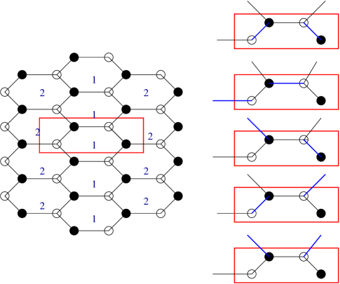
Figure 2: The brane tiling model for the orbifold $\mathbb{C}^{2}/\mathbb{Z}_{2}$. We have also shown the perfect matchings on the right.

The probe D-brane gauge theory can be easily calculated, and it gives the final toric data as in eq. (7) above, with a multiplicity of $2$ being associated to the field $\pmatrix{0\cr 1\cr}$.

This counting is reproduced in fig. (3). Note that there are two distinct edges of the graph (the third edge that describes the redundant third direction). We weigh each edge by the inverse of the rank of the orbifolding group, and associate a weight $\left(\frac{1}{2},0\right)$ and $\left(0,\frac{1}{2}\right)$ to the two distinct edges as shown in figure (3). This counting of the perfect matchings is different from the counting of corresponding quantities in terms of the height function [3]. Our counting proceeds via the edge weight, and directly gives us the closed string twisted sector R charges. Hence, given the quiver gauge theory, and the brane tiling, we can cast the problem of counting perfect matchings to the closed string language and can directly read off the twisted sector charges, and their multiplicities.

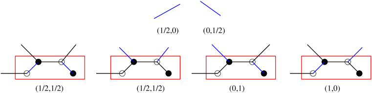
Figure 3: The perfect matchings for the orbifold $\mathbb{C}^{2}/\mathbb{Z}_{2}$. The blue lines on the top indicate the edge weights associated to the two different edges. We have also labeled each perfect matching by the corresponding twisted sector R charge. The redundant matching corresponding to the adjoint field is not shown.

Let us now turn to the orbifold $\mathbb{C}^{2}/\mathbb{Z}_{3}$. In fig. (4) we have shown the brane tiling model for this orbifold and its quiver diagram.

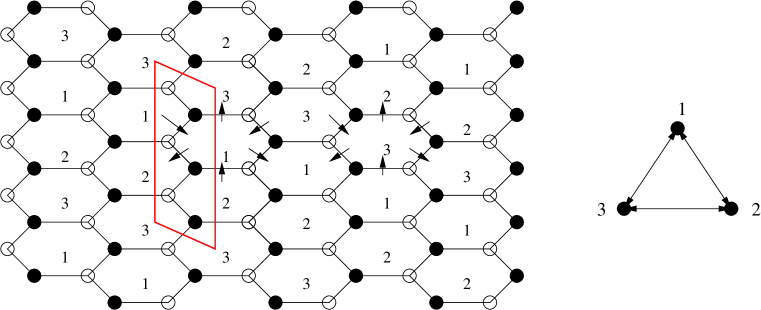
Figure 4: The brane tiling model for the orbifold $\mathbb{C}^{2}/\mathbb{Z}_{3}$ and its quiver diagram without a redundant adjoint field. The fundamental cell in the graph has been marked in red.

Figure (5) shows the perfect matchings for the orbifold $\mathbb{C}^{2}/\mathbb{Z}_{3}$ in the fundamental domain of the tiling.

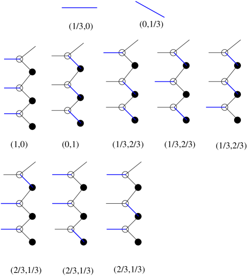
Figure 5: The perfect matchings for the orbifold $\mathbb{C}^{2}/\mathbb{Z}_{3}$. We have not included a final matching involving the redundant edge.

In this case, as before, we have weighted the edges with the (inverse of the) rank of the orbifolding group (except the redundant edge corresponding to the adjoint field) and we have also labeled the perfect matchings in terms of the closed string R charge. We see that the multiplicities of the $\mathbb{C}^{2}/\mathbb{Z}_{3}$ is reproduced in this way of counting, in which we have not made use of the Kasteleyn matrix.

Comparing fig. (3) and fig. (5), we notice a pattern. For any orbifold of the form $\mathbb{C}^{2}/\mathbb{Z}_{n}$, with the rank of the orbifolding group being $n$, the fundamental domain consists of $2n$ points, with $3n$ edges, $n$ of each type, with one type being redundant, corresponding to the unorbifolded $\mathbb{C}$ direction. This means that given an orbifold $\mathbb{C}^{2}/\mathbb{Z}_{n}$, we can engineer its dimer model as follows. We take $n$ edges of two types, the first type having an edge weight $\left(\frac{1}{n},0\right)$ and the other having an edge weight $\left(0,\frac{1}{n}\right)$, with each edge joining two different types of points, which we decide to color white or black. We then make a periodic array using this fundamental unit, and this naturally gives the dimer model for the orbifold $\mathbb{C}^{2}/\mathbb{Z}_{n}$. This procedure is illustrated for the orbifold $\mathbb{C}^{2}/\mathbb{Z}_{5}$ in figs. (6) and (7). In fig. (6), we have illustrated the fundamental unit for the orbifold.

Figure 6: The fundamental unit for $\mathbb{C}^{2}/\mathbb{Z}_{5}$. This contains ten nodes and ten edges.

Fig. (7) shows the emergence of the dimer model for this orbifold on making the fundamental unit periodic.

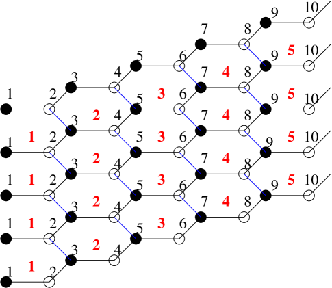
Figure 7: Making the fundamental unit for $\mathbb{C}^{2}/\mathbb{Z}_{5}$ periodic, the dimer model for this orbifold emerges.

Note that this gives us a direct way of relating dimer models with closed string theories and hence to the GLSM. Let us see if we can substantiate this. Consider, eg. the orbifold $\mathbb{C}^{2}/\mathbb{Z}_{3}$. This theory has two marginal twisted sectors, with R charges given by

$$\left(\frac{1}{3},\frac{2}{3}\right),\left(\frac{2}{3},\frac{1}{3}\right)$$ (8)

The toric data for this orbifold is obtained by considering the two dimensional lattice, generated by ${\vec{e}_{1}}=\left(1,0\right)$ and ${\vec{e}_{2}}=\left(0,1\right)$ with these fractional points. Now, restoring integrality in the lattice gives us the toric data for the orbifold,

$${\cal T}=\pmatrix{1&0&-1&-2\cr 0&1&2&3\cr}$$ (9)

The charge matrix for the GLSM for this orbifold is given in a particular basis by

$${\cal T}=\pmatrix{1&2&-3&0\cr 2&1&0&-3\cr}$$ (10)

Hence, the twisted sector R charges, which determine the dimer model for this orbifold is directly related to the GLSM charge matrix. Note also that as mentioned earlier, each perfect matching of the dimer model can be taken to represent a twisted sector in the corresponding closed string theory, i.e a field in the GLSM. Of course, the closed string theory of an orbifold does not see the multiplicities associated with the open string picture. But here we see that in terms of graph theory, the multiplicities actually correspond to various ways of constructing the twisted sector.

Before closing this subsection, let us point out that for supersymmetric $\mathbb{C}^{2}/\mathbb{Z}_{n}$ orbifolds, our construction naturally gives the multiplicities of the GLSM fields as coefficients in the binomial expansion of $(x+y)^{n}$ and the total multiplicity as $2^{n}$, consistent with [18].

3.2 The Partition Function of Perfect Matchings

We now give a mathematical description of the graphical analysis that we have carried out in the last subsection. Let us emphasize that we will not be using the height function [2] in writing down this partition function, but will simply use the properties of the closed string twisted sectors.

It is easy to write down the partition function $P$ of perfect matchings for the supersymmetric orbifolds $\mathbb{C}^{2}/\mathbb{Z}_{n}\times\mathbb{C}$. We will simply write the result here.

$$P=\prod_{i=0}^{n-1}\left(1+\omega^{i}x^{\frac{1}{n}}+\omega^{i}y^{\frac{1}{n}}\right)$$ (11)

where the $1$ appearing in the formula represents the redundant direction which is not taken into account while evaluating the perfect matchings, $\omega=e^{\frac{2\pi i}{n}}$ and we will interpret the product as running over the $(n-1)$ twisted sectors of the orbifold as well as the untwisted sector. The product can be expanded, and gives the multiplicities of the GLSM fields in accordance with [18]. In addition, it indicates the twisted sector R-charges of the blowup modes. Eg. for the case $n=5$, we obtain

$$P=1+x+y+5x^{\frac{1}{5}}y^{\frac{4}{5}}+10x^{\frac{2}{5}}y^{\frac{3}{5}}+10x^{\frac{3}{5}}y^{\frac{2}{5}}+5x^{\frac{4}{5}}y^{\frac{1}{5}}$$ (12)

we note that the powers of $x$ and $y$ reproduce the R-charges of the twisted sector fields. The additional unit term corresponds to the redundant $\mathbb{C}$ direction. From a closed string perspective, these R charges constitute the Newton polygon in the resolution of the singularity $\mathbb{C}^{2}/\mathbb{Z}_{5}$. Note the difference in our formula of eq. (11) and the counting of [3],[4] which uses the height function [2] of perfect matchings for the counting. In this case, the variables $x$ and $y$ have a physical interpretation as representing the two complex directions of $\mathbb{C}^{2}$. By analogy, for the case of the $\mathbb{C}^{3}$ orbifolds, we need three variables. We will see in the next section how this can be nicely interpreted as a supersymmetric completion of non-supersymmetric $\mathbb{C}^{2}$ orbifolds.

According to our discussion in the previous section, for the supersymmetric $\mathbb{C}^{2}/\mathbb{Z}_{5}$ orbifold, the fractional points that need to be added to the $SL(2,Z)$ lattice generated by ${\vec{e}_{1}}=(1,0)$ and ${\vec{e}_{2}}=(0,1)$ are the set of points

$$\left(\frac{1}{5},\frac{4}{5}\right),~{}~{}\left(\frac{2}{5},\frac{3}{5}\right)\left(\frac{3}{5},\frac{2}{5}\right),~{}~{}\left(\frac{4}{5},\frac{1}{5}\right)$$ (13)

In order to restore integrality in this lattice, we pick the points $(\frac{1}{5},\frac{4}{5})$ and $(0,1)$ which we now call ${\vec{e}_{1}}$ and ${\vec{e}_{2}}$ respectively. In terms of these, the precise mapping between the twisted sector charges and the toric data is given by

$$\left(\frac{1}{5},\frac{4}{5}\right)\to\left(1,0\right),~{}~{}\left(\frac{2}{5},\frac{3}{5}\right)\to\left(2,-1\right),~{}~{}$$ (14)

$$\left(\frac{3}{5},\frac{2}{5}\right)\to\left(3,-2\right),~{}~{}\left(\frac{4}{5},\frac{1}{5}\right)\to\left(4,-3\right),~{}~{}$$

With the point ${\vec{e}_{1}}$ being given by $\left(5,-4\right)$ in the new integral lattice. With this mapping, we can identify the points of the toric diagram with the corresponding twisted sectors, and once this is done, eq. (12) reproduces the multiplicities in the probe D-brane picture of the resolution of $\mathbb{C}^{2}/\mathbb{Z}_{5}$.

As another example, consider the supersymmetric orbifold $\mathbb{C}^{2}/\mathbb{Z}_{7}$. The toric data for this orbifolds is given by

$$\mathcal{T}=\pmatrix{1&0&-1&-2&-3&-4&-5&-6\cr 0&1&2&3&4&5&6&7}$$ (15)

For this orbifold, we use eq. (11), with $n=7$ to obtain

$$P=1+x+y+7x^{\frac{6}{7}}y^{\frac{1}{7}}+21x^{\frac{5}{7}}y^{\frac{2}{7}}+35x^{\frac{4}{7}}y^{\frac{3}{7}}+35x^{\frac{3}{7}}y^{\frac{4}{7}}+21x^{\frac{2}{7}}y^{\frac{5}{7}}+7x^{\frac{1}{7}}y^{\frac{6}{7}}$$ (16)

This formula exactly reproduces the twisted sector R charges and their multiplicities in the toric diagram of $\mathbb{C}^{2}/\mathbb{Z}_{7}$.

The advantage of the formula in eq. (11) is that this can be used to compute the multiplicities of the non-supersymmetric $\mathbb{C}^{2}$ orbifolds. As we have mentioned earlier, the gauge theory data for space-time non-supersymmetric orbifolds can be calculated in much the same way as the supersymmetric ones, following the methods of [12] (for non-cyclic orbifolds, see also [19]) From our analysis of the supersymmetric orbifolds above, the procedure is clear for non-supersymmetric orbifolds. We see that the partition function of perfect matchings for the non-supersymmetric $\mathbb{C}^{2}/\mathbb{Z}_{n(p)}$ orbifold is

$$P=\prod_{i=0}^{n-1}\left(1+\omega^{i}x^{\frac{1}{n}}+\omega^{ki}y^{\frac{1}{n}}\right)$$ (17)

where $k<n$ is the smallest integer such that $kp=-1({\rm{mod}}~{}n)$. Let us apply this to the orbifold $\mathbb{C}^{2}/\mathbb{Z}_{5(3)}$. The resolution of this singularity corresponds to turning on two $\mathbb{P}^{1}$s, with self intersection numbers $2$ and $3$, as can be seen from the continued fraction $\frac{5}{3}=2-\frac{1}{3}$. The open string picture of this non-supersymmetric orbifold can be obtained by following the methods outlined in subsection (2.1). The calculations are lengthy to be produced here, and we simply provide the final result for the toric data

$$T=\pmatrix{1&0&-1&-3\cr 0&1&2&5\cr{\bf 1}&{\bf 5}&{\bf 5}&{\bf 1}\cr}$$ (18)

where, in the last row, we have also provided the multiplicities of the GLSM fields.

The closed string picture of this orbifold consists of the two relevant (tachyonic) twisted sectors with R charges $\left(\frac{1}{5},\frac{3}{5}\right),\left(\frac{2}{5},\frac{1}{5}\right)$. The toric data of this orbifold consists of these fractional points in addition with the basis vectors ${\vec{e}_{1}}$ and ${\vec{e}_{2}}$. In order to restore integrality in the lattice, we choose a new basis, and following our convention, we call the point $\left(\frac{1}{5},\frac{3}{5}\right)$ and $\left(0,1\right)$ as our new basis vectors ${\vec{e}_{1}}$ and ${\vec{e}_{2}}$. A simple calculation shows that we then reproduce the data in eq. (18). The partition function of perfect matchings for this orbifold is given by eq. (17) with $n=5,k=3$. Putting these values in eq. (17), we obtain

$$P=1+x+y-5x^{\frac{1}{5}}y^{\frac{3}{5}}+5x^{\frac{2}{5}}y^{\frac{1}{5}}$$ (19)

The above formula (modulo minus signs) precisely reproduces the toric data in eq. (18) along with the relevant twisted sector charges.

As a more complicated example, let us consider the non-supersymmetric orbifold $\mathbb{C}^{2}/\mathbb{Z}_{7(3)}$. The resolution of this orbifold corresponds to the blowup of three $\mathbb{P}^{1}$s with self intersection numbers $(3,2,2)$. In the open string language, the toric data can be calculated using methods outlined in subsection (2.1), and we simply present the final result

$$T=\pmatrix{1&0&-1&-2&-3\cr 0&1&3&5&7\cr{\bf 1}&{\bf 7}&{\bf 14}&{\bf 7}&{\bf 1}}$$ (20)

where in the last line we have given the multiplicities of the GLSM fields that appear in the resolution. This can be obtained from our formula in eq. (18) with $n=7,k=2$ and the partition function is

$$P=1+x+y-7x^{\frac{1}{7}}y^{\frac{3}{7}}+14x^{\frac{3}{7}}y^{\frac{2}{7}}-7x^{\frac{5}{7}}y^{\frac{1}{7}}$$ (21)

this is seen to reproduce the data in eq. (20).

It is not difficult to interpret these results in terms of the perfect matching that we have introduced earlier. The non-supersymmetric orbifolds simply correspond to assigning different weights to the edges of the fundamental cell described earlier. Consider, eg. the orbifold $\mathbb{C}^{2}/\mathbb{Z}_{3}$ of fig. (5). If, instead of weights $\left(\frac{1}{3},0\right),\left(0,\frac{1}{3}\right)$, we assign the weights $\left(\frac{1}{3},0\right),\left(0,\frac{2}{3}\right)$ to the edges of fig. (5), we see that three of the perfect matchings now describe twisted sectors that are irrelevant (i.e the sum of the R-charges exceed unity) and hence need to be projected out of the description of the resolution of the singularity. Only the sector with R-charge $\left(\frac{1}{3},\frac{1}{3}\right)$ is relevant, and this, along with the generators ${\vec{e}_{1}}$ and ${\vec{e}_{2}}$ of the two dimensional lattice describe the Newton polygon for the resolution of the singularity $\mathbb{C}^{2}/\mathbb{Z}_{3(1)}$.

This completes our discussion on generic orbifolds of $\mathbb{C}^{2}$. In the next section, we will focus on orbifolds of $\mathbb{C}^{3}$.

4 Dimers and Closed Strings : The $\mathbb{C}^{3}$ case

In this section, we will deal with supersymmetric orbifolds of $\mathbb{C}^{3}$. We will discuss cyclic as well as non-cyclic orbifolds of $\mathbb{C}^{3}$. We start with the cyclic orbifolds of the form $\mathbb{C}^{3}/\mathbb{Z}_{n}$.

4.1 Cyclic orbifolds of $\mathbb{C}^{3}$

Let us start with the supersymmetric orbifold $\mathbb{C}^{3}/\mathbb{Z}_{3}$. The dimer model and the perfect matchings of this orbifold is shown in fig. (8). We see a familiar pattern from our analysis of the $\mathbb{C}^{2}$ orbifolds. Clearly, counting the number of edges with weights $\left(\frac{1}{3},0,0\right),\left(0,\frac{1}{3},0\right)$ and $\left(0,0,\frac{1}{3}\right)$ (that can be arbitrarily assigned), we find that there are three perfect matchings corresponding to the twisted sector given by the R-charges $\left(\frac{1}{3},\frac{1}{3},\frac{1}{3}\right)$ and the others represent the generators of the unit three dimensional lattice.

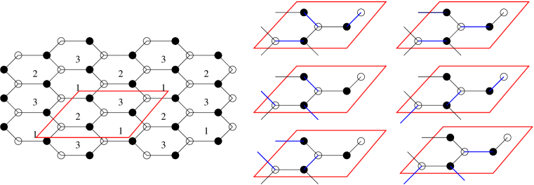
Figure 8: The dimer model and perfect matchings for the supersymmetric orbifold $\mathbb{C}^{3}/\mathbb{Z}_{3}$. The fundamental cell is shown in red.

A similar exercise can be carried out for the case of the orbifold $\mathbb{C}^{3}/\mathbb{Z}_{5}$. The toric data for this orbifold contains two twisted sectors, both of which come with a multiplicity $5$ [12]. We have shown the details of the graphical analysis for this orbifold in figs. (9) and (10).

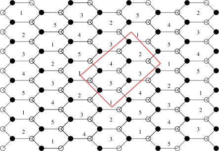
Figure 9: The dimer model for the supersymmetric orbifold $\mathbb{C}^{3}/\mathbb{Z}_{5}$. The fundamental cell is shown in red.

We are now in a position to address the issue of the partition function of perfect matchings for supersymmetric orbifolds of $\mathbb{C}^{3}$. Consider the orbifold $\mathbb{C}^{3}/\mathbb{Z}_{3}$. The partition function

$$P = \prod_{i=0}^{2}\left(x^{\frac{1}{3}}+\omega^{i}y^{\frac{1}{3}}+\omega^{2i}z^{\frac{1}{3}}\right)$$ (22)

$$= x+y+z-3x^{\frac{1}{3}}y^{\frac{1}{3}}z^{\frac{1}{3}}$$

with $\omega=e^{\frac{2\pi i}{3}}$ gives the twisted sector R-charge and the multiplicity of GLSM fields for this orbifold. We interpret this result as the supersymmetric completion of the $\mathbb{C}^{2}/\mathbb{Z}_{3(1)}$ orbifold which is accomplished in this case simply by adding an extra direction parametrized by $x$. We find that this is a generic feature of the supersymmetric cyclic orbifolds of $\mathbb{C}^{3}$, i.e the multiplicities and twisted sector charges are obtained by making a supersymmetric completion of the corresponding non-supersymmetric $\mathbb{C}^{2}$ orbifold.

Next, let us consider the $\mathbb{C}^{3}/\mathbb{Z}_{5}$ orbifold. As is known, this model has two blowup modes corresponding to the two marginal twisted sectors of the closed string SCFT. We take the orbifolding action to be

$$\left(Z_{1},Z_{2},Z_{3}\right)\to\left(\omega Z_{1},\omega^{2}Z_{2},\omega^{2}Z_{3}\right)$$ (23)

where $\omega=e^{\frac{2\pi i}{5}}$. The partition function of perfect matchings is obtained by supersymmetrically completing the $\mathbb{C}^{2}/\mathbb{Z}_{5}$ orbifold. This can be done in three ways, i.e either by completing the $\mathbb{C}^{2}/\mathbb{Z}_{5(1)}$, $\mathbb{C}^{2}/\mathbb{Z}_{5(2)}$ or the $\mathbb{C}^{2}/\mathbb{Z}_{5(3)}$ orbifold. The partition function

$$P=\prod_{i=1}^{2}\left(x^{\frac{1}{5}}+\omega^{i}y^{\frac{1}{5}}+\omega^{ki}z^{\frac{1}{5}}\right)$$ (24)

with $k=2,3,4$ (corresponding to the various non-supersymmetric $\mathbb{C}^{2}/\mathbb{Z}_{5}$ orbifolds) gives the twisted sector charges and the multiplicities of the supersymmetric $\mathbb{C}^{3}$ orbifolds.

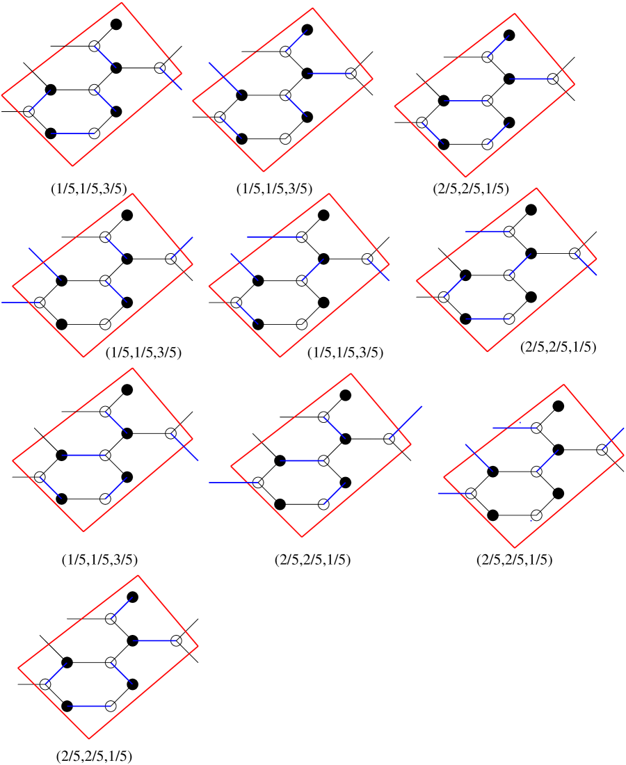
Figure 10: The perfect matchings for the supersymmetric orbifold $\mathbb{C}^{3}/\mathbb{Z}_{5}$. The weights for the edges are $\left(\frac{1}{5},0,0\right),\left(0,\frac{1}{5},0\right),\left(0,0,\frac{1}{5}\right)$. We have not shown the unit vectors in this construction. The red box indicates the fundamental cell which we have retained for convenience.

A more interesting case is the supersymmetric $\mathbb{C}^{3}/\mathbb{Z}_{7}$ orbifold that has two distinct actions

$$\left(Z_{1},Z_{2},Z_{3}\right)\to\left(\omega Z_{1},\omega^{3}Z_{2},\omega^{3}Z_{3}\right)$$

$$\left(Z_{1},Z_{2},Z_{3}\right)\to\left(\omega Z_{1},\omega^{2}Z_{2},\omega^{4}Z_{3}\right)$$ (25)

where $\omega=e^{\frac{2\pi i}{7}}$. In order to obtain the partition function of perfect matchings, we could supersymmetrically complete the non-supersymmetric orbifold $\mathbb{C}^{2}/\mathbb{Z}_{7(3)}$, in which case we will obtain the supersymmetric orbifold $\mathbb{C}^{3}/\mathbb{Z}_{7}$ with the orbifolding action being the first one of eq. (25), or we could do the same with the orbifold $\mathbb{C}^{2}/\mathbb{Z}_{7(2)}$ for which the second action of eq. (25) is obtained (other orbifold actions of $\mathbb{C}^{2}/\mathbb{Z}_{7}$ give permutations of these results).

Consider eq. (17) with $n=7$ and $k=2$. This gives the orbifold $\mathbb{C}^{2}/\mathbb{Z}_{7(3)}$. Completing this partition function amounts to the new function

$$P=\prod_{i=0}^{4}\left(x^{\frac{1}{7}}+\omega^{i}y^{\frac{1}{7}}+\omega^{2i}z^{\frac{1}{7}}\right)$$ (26)

Expanding this, we obtain

$$P=x+y+z-7x^{\frac{1}{7}}y^{\frac{5}{7}}z^{\frac{1}{7}}+14x^{\frac{2}{7}}y^{\frac{3}{7}}z^{\frac{2}{7}}+-7x^{\frac{3}{7}}y^{\frac{1}{7}}z^{\frac{3}{7}}$$ (27)

This gives the multiplicities and twisted sector charges of the orbifold as in the first of eq. (25). Similarly, completing eq. (17) with $n=7$ and $k=3$ can be seen to reproduce the twisted sector charges and the multiplicities of the second orbifold action of eq. (25). A similar analysis can be done for higher rank orbifolds of $\mathbb{C}^{3}$ and the results follow the same pattern as presented here. We now go over to a discussion of supersymmetric orbifolds of the form $\mathbb{C}^{3}/\mathbb{Z}_{n}\times\mathbb{Z}_{m}$.

4.2 Non-cyclic orbifolds of $\mathbb{C}^{3}$

In this subsection, we briefly discuss how our methods apply to the orbifolds of $\mathbb{C}^{3}$ of the form $\mathbb{C}^{3}/\mathbb{Z}_{n}\times\mathbb{Z}_{m}$. We concentrate on the simplest example, i.e for $n=m=2$, since the higher rank orbifolds of this class have large multiplicities and are difficult to present graphically. For the $\mathbb{C}^{3}/\mathbb{Z}_{2}\times\mathbb{Z}_{2}$ orbifold, we have presented the dimer model and the perfect matchings in fig. (11). Clearly, we see that our results of the last section can be adapted to this case with ease. In this case, we weigh the edges by weights $\left(\frac{1}{2},0,0\right),\left(0,\frac{1}{2},0\right)$ and $\left(0,0,\frac{1}{2}\right)$. This correctly gives us the twisted sector charges and the multiplicities of the orbifold [14],[19].

We can address the issue of partial resolution of singularities here. This would corresponding to removing certain corners of the toric diagram. This can be visualised in the following way : we choose the corner to be resolved and identify the corresponding perfect matching. Then we choose any one of the edges of this matching (that has to be removed) and project out any other diagram that involves the said edge.

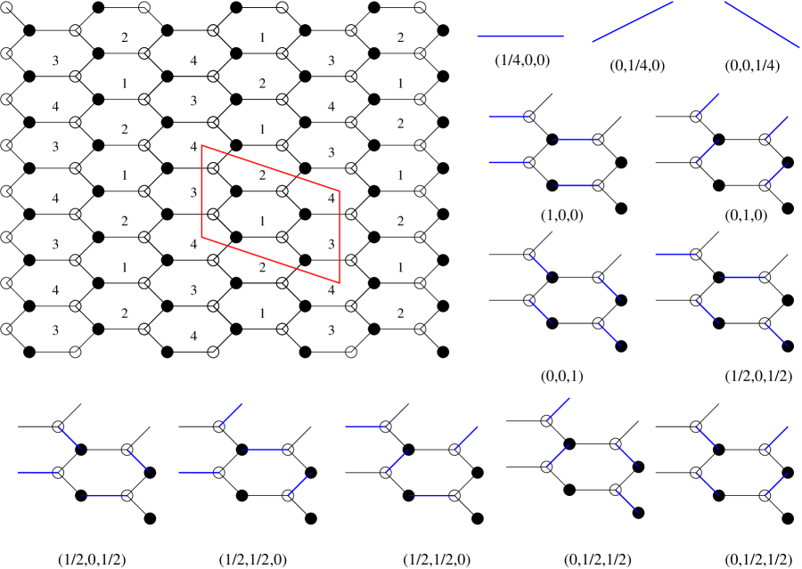
Figure 11: The dimer model and perfect matchings for the supersymmetric orbifold $\mathbb{C}^{3}/\mathbb{Z}_{2}\times\mathbb{Z}_{2}$.

Eg. in fig. (11), suppose we twisted sector corresponding to the weight $\left(0,1,0\right)$. From the perfect matching corresponding to this weight, we choose any edge and remove all diagrams that contains this edge in its perfect matching. The twisted sector corresponding to the charges $\left(\frac{1}{2},0,\frac{1}{2}\right)$ is unaffected whereas one each of the perfect matchings corresponding to the charges $\left(\frac{1}{2},\frac{1}{2},0\right)$ and $\left(0,\frac{1}{2},\frac{1}{2}\right)$ are seen to be “resolved,” and finally we get precisely the toric diagram with the multiplicities of the SPP singularity [14]. We leave a detailed study of the phenomena of partial resolutions to a future work.

5 Conclusions

In this paper, we have explored the connection between dimer models that naturally arise in the study of D-brane gauge theories, and closed string theories. We have seen that by weighing the edges of the perfect matchings of bipartite graphs, we are able to give an interpretation of these perfect matchings as twisted sector states of closed strings on orbifolds. Since each perfect matching is a twisted sector state, this gives an explanation of the dimer-GLSM correspondence, complementary to the methods used in [8]. Further, we emphasize that this extends the correspondence to non-supersymmetric orbifolds (of $\mathbb{C}^{2}$) as well. Note that in our description, we have not used the height function as in previous works, but have established a direct connection with twisted sector R charges via a counting of weighted edges.

There are various issues yet to understand. The first question that one might ask is whether there is an analogue of brane tiling corresponding to non-supersymmetric graphs. This issue can be addressed as follows. Non-supersymmetric orbifolds of $\mathbb{C}^{2}$ can be obtained from supersymmetric orbifolds of $\mathbb{C}^{3}$ by a method inverse to that of supersymmetric completion [20]. This can be simply understood with an example. Consider, eg. the supersymmetric orbifold $\mathbb{C}^{3}/\mathbb{Z}_{5}$, with the orbifolding action being

$$\left(Z_{1},Z_{2},Z_{3}\right)\to\left(\omega Z_{1},\omega Z_{2},\omega^{3}Z_{3}\right)$$ (28)

where $\omega=e^{\frac{2\pi i}{5}}$. A resolution of this supersymmetric $\mathbb{C}^{3}$ orbifold can be obtained by considering three non-supersymmetric $\mathbb{C}^{2}$ orbifolds, namely $\mathbb{C}^{2}/\mathbb{Z}_{5(1)}$, $\mathbb{C}^{2}/\mathbb{Z}_{5(2)}$ and $\mathbb{C}^{2}/\mathbb{Z}_{5(3)}$. The toric data of the resolution of $\mathbb{C}^{3}/\mathbb{Z}_{5}$ can then be constructed by gluing the data for these three $\mathbb{C}^{2}$ orbifolds. This procedure has been dubbed the “champions meet” in [20]. Proceeding in the reverse direction, it seems that an analogue of the brane tiling model for a non-supersymmetric $\mathbb{C}^{2}$ orbifold can be obtained from a supersymmetric $\mathbb{C}^{3}$ brane tiling by removing one of the $\mathbb{C}^{3}$ directions, which corresponds to removing one row from the charge matrix for the quiver diagram of the orbifold. However, as one can check, this procedure does not provide a consistent tiling with bipartite graphs, but rather one has to consider a tripartite graph. A possible clue is that the gluing rules of [20], when translated in the language of graphs, might give us further hints as to what is the analogue of brane tilings for non-supersymmetric orbifolds. This issue is under investigation.

The issue of non-supersymmetric $\mathbb{C}^{3}$ orbifolds (which might have terminal singularities) is also a interesting direction of future work. This will presumably involve construction of supersymmetric $\mathbb{C}^{4}$ orbifolds, and then using methods developed in this papr. We leave these issues to a future work.

Acknowledgments

It is a pleasure to thank Ami Hanany and for various useful discussions and email correspondence. Thanks are due to V. Subrahmanyam for lively discussions on dimer models.

References

- [1] P. Kasteleyn, “Graph theory and crystal physics,” in Graph theory and theoretical physics, pp 43 - 110, Academic Press, London, 1967.
- [2] R. Kenyon, “An introduction to the dimer model,” math.CO/0310236
- [3] A. Hanany, K. D. Kennaway, “Dimer models and toric diagrams,” hep-th/0503149
- [4] S. Franco, A. Hanany, K. D. Kennaway, D. Vegh, B. Wecht, “ Brane dimers and quiver gauge theories,” JHEP 0601 2006, 096
- [5] S. Franco, A. Hanany, D. Martelli, J. Sparks, D. Vegh, B. Wecht, “ Gauge theories from toric geometry and brane tilings,” JHEP 0601 (2006) 128
- [6] B. Feng, Y-H He, K. D. Kennaway, C. Vafa, “ Dimer models from mirror symmetry and quivering amoebae,” hep-th/0511287
- [7] E. Witten, “Phases of theories in two dimensions,” Nucl. Phys. B403 (1993) 159, hep-th/9301042
- [8] S. Franco, D. Vegh, “ Moduli spaces of gauge theories from dimer models: Proof of the correspondence,” JHEP 0611 (2006) 054, hep-th/0601063
- [9] M. R. Douglas, G. Moore, “ D-branes, quivers, and ALE instantons,” hep-th/9603167
- [10] C. V. Johnson, R. C. Myers, “Aspects of type IIB theory on ALE spaces,” Phys. Rev. D55 (1997) 6382, hep-th/9610140
- [11] Y-H He, “ Lectures on D-branes, gauge theories and Calabi-Yau singularities,” hep-th/0408142
- [12] M. R. Douglas, B. R. Greene, D. R. Morrison, “Orbifold resolution by D-branes,” Nucl. Phys. B506 (1997) 84, hep-th/9704151
- [13] T. Sarkar, “Brane probes, toric geometry, and closed string tachyons,” Nucl. Phys. B648 497 (2003), hep-th/0206109.
- [14] B. Feng, A. Hanany, Y-H He, “ D-brane gauge theories from toric singularities and toric duality,” Nucl. Phys. B595 (2001) 165, hep-th/0003085
- [15] M. Reid, “Young person’s guide to Canonical Singularities,” Proc. Symp. Pure Math., 46 (1987) 345.
- [16] P. S. Aspinwall, B. R. Greene, “ On the geometric interpretation of superconformal theories,” Nucl.Phys. B 437 (1995) 205, hep-th/9409110.
- [17] T. Sarkar, “ On Tachyons in Generic Orbifolds of and Gauged Linear Sigma Models,” JHEP 0702 (2007) 025, hep-th/0612046.
- [18] B. Feng, S. Franco, A. Hanany, Y-H He, “Symmetries of toric duality,” JHEP 0212 (2002) 076, hep-th/0205144.
- [19] T. Sarkar, D-brane gauge theories from toric singularities of the form and ,” Nucl. Phys. B595 (2001) 201, hep-th/0005166.
- [20] A. Craw, M. Reid, “How to calculate A-Hilb ,” math.AG/9909085.