The Calibration of Mid–Infrared Star Formation Rate Indicators.

Abstract

With the goal of investigating the degree to which the mid–infrared emission traces the star formation rate (SFR), we analyze Spitzer 8 $\mu$m and 24 $\mu$m data of star–forming regions in a sample of 33 nearby galaxies with available HST/NICMOS images in the Pa$\alpha$ ($\lambda$1.8756 $\mu$m) emission line. The galaxies are drawn from the SINGS sample, and cover a range of morphologies and a factor $\sim$10 in oxygen abundance. Published data on local low–metallicity starburst galaxies and Luminous Infrared Galaxies are also included in the analysis. Both the stellar–continuum–subtracted 8 $\mu$m emission and the 24 $\mu$m emission correlate with the extinction–corrected Pa$\alpha$ line emission, although neither relationship is linear. Simple models of stellar populations and dust extinction and emission are able to reproduce the observed non–linear trend of the 24 $\mu$m emission versus number of ionizing photons, including the modest deficiency of 24 $\mu$m emission in the low metallicity regions, which results from a combination of decreasing dust opacity and dust temperature at low luminosities. Conversely, the trend of the 8 $\mu$m emission as a function of the number of ionizing photons is not well reproduced by the same models. The 8 $\mu$m emission is contributed, in larger measure than the 24 $\mu$m emission, by dust heated by non–ionizing stellar populations, in addition to the ionizing ones, in agreement with previous findings. Two SFR calibrations, one using the 24 $\mu$m emission and the other using a combination of the 24 $\mu$m and H$\alpha$ luminosities (Kennicutt et al., 2007a), are presented. No calibration is presented for the 8 $\mu$m emission, because of its significant dependence on both metallicity and environment. The calibrations presented here should be directly applicable to systems dominated by on–going star formation.

1 Introduction

The multi–wavelength galaxy surveys of unprecedented angular resolution recently made available by combined space (HST, Spitzer) and ground–based observations are providing for the first time the tools to cross–calibrate star formation rate (SFR) indicators at different wavelengths, and to test the physical assumptions underlying each indicator.

Easy accessibility has traditionally favored the use of the ultraviolet (UV) stellar continuum and of the optical nebular recombination lines as SFR indicators, the former mainly in the intermediate–high redshift regime (as it gets redshifted into the optical observer frame) and the latter mostly in low–redshift surveys. Both indicators only probe the stellar light that emerges from a galaxy unabsorbed by dust. The UV is heavily affected by dust attenuation, and numerous efforts have attempted to find general tools to mitigate the effects of dust on this important SFR indicator (e.g., Calzetti, Kinney & Storchi–Bergmann, 1994; Kennicutt, 1998a; Meurer, Heckman & Calzetti, 1999; Hopkins et al., 2001; Sullivan et al., 2001; Buat et al., 2002, 2005; Bell, 2003; Hopkins, 2004; Salim et al., 2007). Cross–calibrations with optical recombination lines and other indicators have also attempted to account for the $\sim$10 times or more longer stellar timescales probed by the UV relative to tracers of ionizing photons (e.g., Sullivan et al., 2001; Kong et al., 2004; Calzetti et al., 2005). Among the recombination lines, H$\alpha$ is the most widely used, due to a combination of its intensity and a lower sensitivity to dust attenuation than bluer nebular lines. Although to a much lesser degree than the UV, the H$\alpha$ line is still affected by dust attenuation, plus is impacted by assumptions on the underlying stellar absorption and on the form of the high end of the stellar initial mass function (e.g., Calzetti, Kinney & Storchi–Bergmann, 1994; Kennicutt, 1998a; Hopkins et al., 2001; Sullivan et al., 2001; Kewley et al., 2002; Rosa–Gonzalez, Terlevich & Terlevich, 2002).

Infrared SFR indicators are complementary to UV–optical indicators, because they measure star formation via the dust–absorbed stellar light that emerges beyond a few $\mu$m. Although SFR indicators using the infrared emission had been calibrated during the IRAS times (e.g., Lonsdale Persson & Helou, 1987; Rowan–Robinson & Crawford, 1989; Sauvage & Thuan, 1992), interest in the this wavelength range had been rekindled in more recent times by the discovery of submillimeter–emitting galaxy populations at cosmological distances (e.g., Smail, Ivison & Blain, 1997; Hughes et al., 1998; Barger et al., 1998; Eales et al., 1999; Chapman et al., 2005). In dusty starburst galaxies, the bolometric infrared luminosity L_IR in the $\sim$3–1100 $\mu$m window is directly proportional to the SFR ( e.g., Kennicutt, 1998a). However, even assuming that most of the luminous energy produced by recently formed stars is re-processed by dust in the infrared, at least two issues make the use of this SFR indicator problematic. (1) Evolved, i.e., non-star-forming, stellar populations also heat the dust that emits in the IR wavelength region, thus affecting the calibration of SFR(IR) in a stellar-population-dependent manner (e.g., Lonsdale Persson & Helou, 1987; Helou, 1986; Kennicutt, 1998a). (2) In intermediate/high redshift studies, the bolometric infrared luminosity is often extrapolated from measurements at sparsely sampled wavelengths, most often in the sub–mm and radio observer’s frame (e.g., Smail, Ivison & Blain, 1997; Chapman et al., 2005), and such extrapolations are subject to many uncertainties.

The interest in calibrating monochromatic mid-infrared SFR diagnostics stems from their potential application to both the local Universe and intermediate and high redshift galaxies observed with Spitzer and future infrared/submillimeter missions (Daddi et al., 2005; Wu et al., 2005). One such application is the investigation of the scaling laws of star formation in the dusty environments of galaxy centers (Kennicutt, 1998b; Kennicutt et al., 2007a). The use of monochromatic (i.e., one band or wavelength) infrared emission for measuring SFRs offers one definite advantage over the bolometric infrared luminosity: it removes the need for highly uncertain extrapolations of the dust spectral energy distribution across the full wavelength range. Over the last few years, a number of efforts have gone into investigating the potential use of monochromatic infrared emission for measuring SFRs.

Early studies employing ISO data have not resolved whether the warm dust and aromatic bands emission around 8 $\mu$m can be effectively used as a SFR indicator, since different conclusions have been reached by different authors. Roussel et al. (2001) and Förster Schreiber et al. (2004) have shown that the emission in the 6.75 $\mu$m ISO band correlates with the number of ionizing photons (SFR) in galaxy disks and in the nuclear regions of galaxies. Conversely, Boselli, Lequeux & Gavazzi (2004) have found that the mid–IR emission in a more diverse sample of galaxies (types Sa through Im–BCDs) correlates more closely with tracers of evolved stellar populations not linked to the current star formation. Additionally, Haas, Klaas & Bianchi (2002) find that the ISO 7.7 $\mu$m emission is correlated with the 850 $\mu$m emission from galaxies, suggesting a close relation between the ISO band emission and the cold dust heated by the general (non–star–forming) stellar population. This divergence of results highlights the multiplicity of sources for the emission at 8 $\mu$m (e.g., Peeters, Spoon & Tielens, 2004; Tacconi–Garman et al., 2005), as well as the limits in the ISO angular resolution and sensitivity for probing a sufficiently wide range of galactic conditions.

The emission in the 8 $\mu$m and other MIR bands is generally attributed to Polycyclic Aromatic Hydrocarbons (PAH, Leger & Puget, 1984; Sellgren, 1984; Allamandola, Tielens & Barker, 1985; Sellgren, Luan & Werner, 1990), large molecules transiently heated by single UV and optical photons in the general radiation field of galaxies or near B stars (Li & Draine, 2002; Haas, Klaas & Bianchi, 2002; Boselli, Lequeux & Gavazzi, 2004; Peeters, Spoon & Tielens, 2004; Wu et al., 2005; Mattioda et al., 2005), and which can be destroyed, fragmented, or ionized by harsh UV photon fields (Boulanger et al., 1988, 1990; Helou, Ryter & Soifer, 1991; Houck et al., 2004; Pety et al., 2005). Spitzer data of the nearby galaxies NGC300 and NGC4631 show that 8 $\mu$m emission highlights the rims of HII regions and is depressed inside the regions, indicating that the PAH dust is heated in the PDRs surrounding HII regions and is destroyed within the regions (Helou et al., 2004; Bendo et al., 2006). Analysis of the mid–IR emission from the First Look Survey (Fang et al., 2004) galaxies shows that the correlation between the Spitzer 8 $\mu$m band emission and tracers of the ionizing photons is shallower than unity (Wu et al., 2005), in agreement with the correlations observed for HII regions in the nearby, metal–rich, star–forming galaxy NGC5194 (M51a Calzetti et al., 2005).

The 24 $\mu$m emission is a close tracer of SFR in the dusty center of NGC5194 (Calzetti et al., 2005) and in NGC3031 (Perez–Gonzalez et al., 2006). The general applicability of this monochromatic indicator has so far been explored only for a small number of cases, mostly bright galaxies (e.g., Wu et al., 2005; Alonso–Herrero et al., 2006). A potential complication is that most of the energy from dust emerges at wavelengths longer than $\sim$40–50 $\mu$m (see Dale et al., 2006, and references therein). Thus the mid–IR does not trace the bulk of the dust emission, and, because it lies on the Wien side of the blackbody spectrum, could be sensitive to the dust temperature rather than linearly correlating with source luminosity.

This study investigates the use of the Spitzer IRAC 8 $\mu$m and MIPS 24 $\mu$m monochromatic luminosities as SFR indicators for star forming regions in a subsample of the SINGS galaxies (SINGS, or the Spitzer Infrared Nearby Galaxies Survey, is one of the Spitzer Legacy Programs, Kennicutt et al., 2003). Star–forming regions in galaxies represent a first stepping–stone for characterizing SFR indicators, as they can be considered simpler entities than entire galaxies.

We also extend our analysis to include both new and published integrated (galaxy–wide) data on local low–metallicity starburst galaxies (Engelbracht et al., 2005) and Luminous Infrared Galaxies (LIRGs, Alonso–Herrero et al., 2006). These data are used to explore whether the relationships derived for the star–forming regions that constitute our main sample are applicable to starburst–dominated galaxies as a whole. A future paper will investigate the viability of the mid–infrared luminosities as SFR tracers for more general classes of galaxies (Kennicutt & Moustakas, 2006).

The Spitzer observations are coupled with near–infrared HST/NICMOS observations centered on the Paschen–$\alpha$ hydrogen emission line (Pa$\alpha$, at 1.8756 $\mu$m), and with ground–based H$\alpha$ observations obtained by the SINGS project. The hydrogen emission lines trace the number of ionizing photons, and the Pa$\alpha$ line is only modestly impacted by dust extinction. Furthermore, the Pa$\alpha$ and H$\alpha$ lines are sufficiently separated in wavelength that reliable extinction corrections can be measured (Quillen & Yukita, 2001). Because of its relative insensitivity to dust extinction (less than a factor of 2 correction for the typical extinction in our galaxies, A${}_{V}\lesssim$5 mag), Pa$\alpha$ represents a nearly unbiased tracer of the current SFR over a timescale of about 10 Myr (Kennicutt, 1998a). The access to Pa$\alpha$ images to use as a yardstick for calibrating the mid–infrared emission is the basic motivation for the present work.

The present paper is organized as follows: Section 2 introduces the sample of local star–forming galaxies from SINGS; Section 3 presents the data, while the measurements used in the analysis are presented in Section 4. Section 5 briefly introduces the low metallicity starburst galaxies from Engelbracht et al. (2005) and the LIRGs from Alonso–Herrero et al. (2006). The main findings are reported in Section 6, and the comparison with models is made in Section 7. Discussion and a summary are given in Sections 8 and 9, respectively. Details on the models of dust absorption and emission are in the Appendix.

2 Main Sample Description

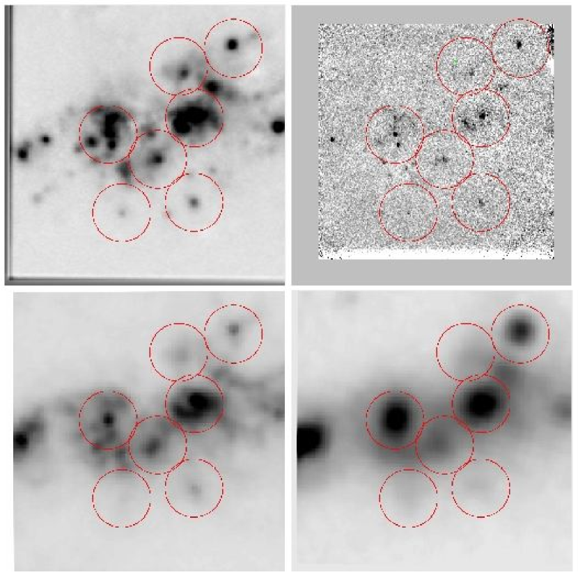
Figure 1: Example of aperture selection in one of our fields. The central $\sim$1^′ of the galaxy NGC0925 is shown at H$\alpha$ (top–left), Pa$\alpha$ (top–right), stellar–continuum–subtracted 8 $\mu$m (bottom–left), and 24 $\mu$m (bottom–right). The 13^′′ apertures used for photometric measurements are shown as red circles, and correspond to physical sizes of $\sim$580 pc. The field shown is one of the two obtained in the central region of this galaxy. North is up; East is left.

The SINGS sample of 75 galaxies (Kennicutt et al., 2003) was used as our baseline sample for which HST observations in the infrared were either obtained as part of our project or retrieved from the HST archive (see details in section 3.2). The only criterion required for a SINGS galaxy to be observed with the HST was to have a redshifted Pa$\alpha$ emission within the transmission curve of one of the NICMOS narrowband filters. A total of 39 galaxies, or 52% of the SINGS sample, were observed in the Pa$\alpha$ line (example in Figure 1). The HST/NICMOS–observed galaxies are fully representative of the SINGS sample as a whole, in terms of morphological types, range of metallicity, and SFRs.

The infrared data of 4 of the 39 galaxies show non–recoverable problems (see section 3.2 for additional explanation); two more galaxies, M81DwA and DDO154 do not show either optical line emission or mid–IR dust emission in the region imaged in the near–infrared with HST. All six galaxies were discarded from the current analysis, thus leaving a net sample of 33 galaxies. Table 1 lists the main characteristics of the 39 galaxies, separating the discarded ones from the remainder of the sample.

The 33 galaxies are divided in three groups according to their oxygen abundance: high metallicity galaxies (12$+$log(O/H)$>$8.35), medium metallicity galaxies (8.00$<$12$+$log(O/H)$\lesssim$8.35), and low metallicity galaxies (12$+$log(O/H)$\lesssim$8.00). The two sets of disk-averaged oxygen abundance values listed in Table 1 differ systematically by about 0.6 dex (Moustakas et al., 2007). As described by Moustakas et al. (2007), the set of lower numbers for the oxygen abundance is roughly tied to the electron temperature abundance scale (Pilyugin & Thuan, 2005), while the higher abundance set is based on stellar populations plus photoionization modelling (Kobulnicky & Kewley, 2004; Kewley & Dopita, 2002). The difference between the two scales is due to a as–yet unidentified systematic zeropoint offset, and the ‘true’ oxygen abundance should lie somewhere between the two listed values; however, the relative ranking of abundances on either of the scales should be fairly accurate. On this basis, we assign a galaxy into a metallicity bin based on the average of the two values. Metallicity gradients across galaxies are likely of little impact in our analysis. The observations probe the inner $\approx$0.8–5.1 kpc, depending on the distance; typical metallicity variations over these region sizes are less than $\sim$0.3 dex for our spiral galaxies (Moustakas et al., 2007), and therefore are not expected to play a significant role in our results.

Within the area imaged by the HST/NICMOS for each galaxy in the main sample (Table 1), regions of star formation are identified and their fluxes measured over typical sizes of $\sim$200–600 pc (section 4 and Figure 1). These regions are termed here ‘HII knots’, and they are far simpler units, in terms of stellar population and star formation history, than whole galaxies. The HII knots in this study cannot be considered individual HII regions in the strict meaning of the term. Limitations in angular resolution, as discussed in section 4, force us to consider areas within galaxies which may be populated by multiple HII regions. The main requirement is for such areas to be local peaks of current star formation, as determined from hydrogen line or infrared emission. The ionizing populations in these regions can be approximated as having comparable ages, and more evolved stellar populations do not tend to dominate the radiation output. Although caution should be used when deriving a star formation rate for quasi–single–age populations, the investigation of simpler, star–formation–dominated structures should offer better insights than whole galaxies on the strengths and weaknesses of the mid–infrared SFR indicators of interest here.

Details on the low–metallicity starburst galaxies from Engelbracht et al. (2005) and on the LIRGs from Alonso–Herrero et al. (2006) are given in section 5.

3 Observations and Data Reduction

3.1 Spitzer IRAC and MIPS Imaging Data

Spitzer images for the galaxies in Table 1 were obtained with both IRAC (3.6, 4.5, 5.8, and 8.0 $\mu$m) and MIPS (24, 70, and 160 $\mu$m), as part of the SINGS Legacy project, between $\sim$March 2004 and $\sim$August 2005. A description of this project and the observing strategy can be found in Kennicutt et al. (2003).

Each galaxy was observed twice in each of the four IRAC bands, with a grid covering the entire galaxy and the surrounding sky. The observing strategy allowed a separation of a few days between the two observations to enable recognition and exclusion of asteroids and detector artifacts. Total exposure times in each filter are 240 s in the center of the field, and 120 s along the grids’ edges. The SINGS IRAC pipeline was used to create the final mosaics, which exploits the sub-pixel dithering to better sample the emission, and resamples each mosaic into 0.75^′′ pixels (Regan et al., 2004). The measured 8 $\mu$m PSF FWHM is, on average, 1.9^′′, and the 1 $\sigma$ sensitivity limit in the central portion of the 8 $\mu$m mosaic is 1.2$\times$10^-6 Jy arcsec^-2.

As the interest in this paper is in using the dust emission at mid–infrared wavelengths (8 $\mu$m and 24 $\mu$m) as SFR tracers, we need to remove the stellar continuum contribution from the 8 $\mu$m images. This contribution is, in general, small in high metallicity, dusty galaxies (e.g., Calzetti et al., 2005), but can become significant in lower metallicity, and more dust–poor galaxies. ‘Dust–emission’ images at 8 $\mu$m are obtained by subtracting the stellar contribution using the recipe of Helou et al. (2004):

$$f_{8\mu m,\ dust}(\nu)=f_{8\mu m}(\nu)-\beta f_{3.6\mu m}(\nu),$$ (1)

where the coefficient $\beta$ is in the range 0.22–0.29, as determined from isolated stars in the galaxies’ fields. Visual inspection of the stellar–continuum subtracted images suggests that this approach is fairly accurate in removing stellar emission; occasional foreground stars located along the galaxies’ lines of sight are in general removed by this technique. Although the 3.6 $\mu$m images can include, in addition to photospheric emission from stars, a component of hot dust emission, this component is unlikely to have an impact beyond a few percent on the photometry of the dust–only 8 $\mu$m images (Calzetti et al., 2005).

MIPS observations of the galaxies were obtained as scan maps, with enough coverage to include surrounding background in addition to the galaxy. The reduction steps for MIPS mosaics are described in Gordon et al. (2005) and Bendo et al. (2006). At 24 $\mu$m, the PSF FWHM is $\sim$5.7^′′, and the 1 $\sigma$ detection limit is 1.1$\times$10^-6 Jy arcsec^-2. The MIPS images are considered ‘dust’ images for all purposes, as contributions from the photospheric emission of stars and from nebular emission are negligible (a few percent) at these wavelengths.

3.2 HST Imaging Data

The main advantage of using near–infrared narrowband imaging, rather than spectroscopy, is the potential of capturing, in principle, all of the light in the Pa$\alpha$ line, thus enabling a more secure measurement of the total line emission from the targets. The HST/NICMOS narrowband filters of interest here have $\sim$1% band–passes, that can easily accommodate gas line emission with a few hundred km/s shift relative to the galaxy’s systemic velocity.

Most of the HST/NICMOS observations for the galaxies in our sample come from the HST SNAP program 9360 (P.I.: Kennicutt). For 9 of the galaxies, archival HST data were used, from programs GO-7237 and SNAP-7919.

Observations for SNAP-9360 were obtained with the NIC3 camera, in the narrowband filters F187N, F190N (Pa$\alpha$ emission line at restframe wavelength $\lambda$=1.8756 $\mu$m and adjacent stellar continuum), and the broadband filter F160W. The NIC3 camera has a field of view of 51^′′, and observations were obtained with 4 dithered pointings along a square pattern with 0.9^′′ sides, to better remove cosmic rays and bad pixels. Thus, NICMOS observations imaged the central $\lesssim$1 arcmin of each galaxy. The NIC3 0^′′.2 pixels undersample the NICMOS PSF, although this is not a concern for the diffuse ionized gas emission. On–target total exposure times were 640 s, 768 s, and 96 s, for F187N, F190N, and F160W, respectively.

The data were reduced with the STScI IRAF/STSDAS pipeline calnica, which removes instrumental effects, bad pixels, and cosmic rays, and produces images in count–rate units. The removal of the quadrant-dependent ‘pedestal’ was done with the IRAF/STSDAS routine pedsub. The four dithered exposures were combined with the IRAF/STSDAS mosaicing pipeline calnicb.

For our analysis, only the two narrowband images are used, and the emission line–only images are obtained by subtracting the continuum–only images, rescaled by the ratio of the filters’ efficiencies, from the line$+$continuum image. Program 9360 was executed after the NICMOS Cryocooler System (NCS) had been installed on the HST, providing a detector quantum efficiency about 30% higher in the H-band than during pre–NCS (i.e., pre–2002) operations. This is an important difference when comparing depths of SNAP–9360 with those of the archival NICMOS images, which were obtained pre–NCS. The average 1 $\sigma$ sensitivity limit of the continuum–subtracted image is 6.4$\times$10^-17 erg s^-1 cm^-2 arcsec^-2. In units that will be easier to relate to the analysis performed in this paper, our 1 $\sigma$ limit for a specific Pa$\alpha$ luminosity measured in a 13^′′–diameter aperture is 2.83$\times$10³⁷ erg s^-1 kpc^-2; in a 50^′′–diameter aperture, the 1 $\sigma$ limit is 1.04$\times$10³⁸ erg s^-1 kpc^-2 .

The archival NICMOS data from HST snapshot program 7919 are described in Böker et al. (1999). Here we summarize the main differences with SNAP–9360. Data for the SNAP–7919 were obtained with a single pointing (and a single integration) of the galaxy’s center with the NIC3 camera. One narrowband filter (F187N or F190N depending on redshift) and the broadband F160W filter were used, for $\sim$768 s and 192 s, respectively. We re-processed the archival images through calnica, to improve the removal of instrumental effects and of cosmic rays by using a more recent version of the calibration pipeline than the one used in Böker et al. (1999); the quadrant–dependent pedestal was removed with pedsub. As in Böker et al. (1999), the rescaled broadband filter is used for removal of the underlying stellar continuum from the image containing the Pa$\alpha$ emission line. The images from SNAP–7919 are deeper than in SNAP–9360, with an average 1 $\sigma$ sensitivity limit of the continuum–subtracted image of 3.5$\times$10^-17 erg s^-1 cm^-2 arcsec^-2.

Broadband filters may not provide the optimal underlying stellar continuum signature, especially if uneven dust extinction in the galaxy produces color variations within the filter’s bandpass. To check the impact of this potential effect, we have compared observations of galaxies in common between the SNAP–9360 and SNAP–7919 programs: NGC3184, NGC4826, NGC5055, and NGC6946 (images of NGC0925 are also present in both programs, but the pointings are only partially overlapping, and are sufficiently different that both images are used in our analysis, see Table 1). For SNAP–9360, two narrowband images are available, thus yielding a ‘cleaner’ line image. Comparison of continuum–subtracted images in both programs for regions in the common galaxies yields differences in the Pa$\alpha$ photometry in the range 10%–30%, which is in general well within our random uncertainty for the Pa$\alpha$ measurements (section 4.2).

The NICMOS archival data for NGC5194 (HST program 7237) are described in Scoville et al. (2001) and Calzetti et al. (2005). The main difference with the data in 9360 is that the NGC5194’s image is a 3$\times$3 NIC3 mosaic that spans the central 144^′′ arcsec². Each pointing was observed in both F187N and F190N, with 128 s exposure times. The sensitivity is variable, being lower at the seams of the 9 images that form the mosaic. The average 1 $\sigma$ sensitivity limit of the continuum–subtracted image for this galaxy is 1.8$\times$10^-16 erg s^-1 cm^-2 arcsec^-2.

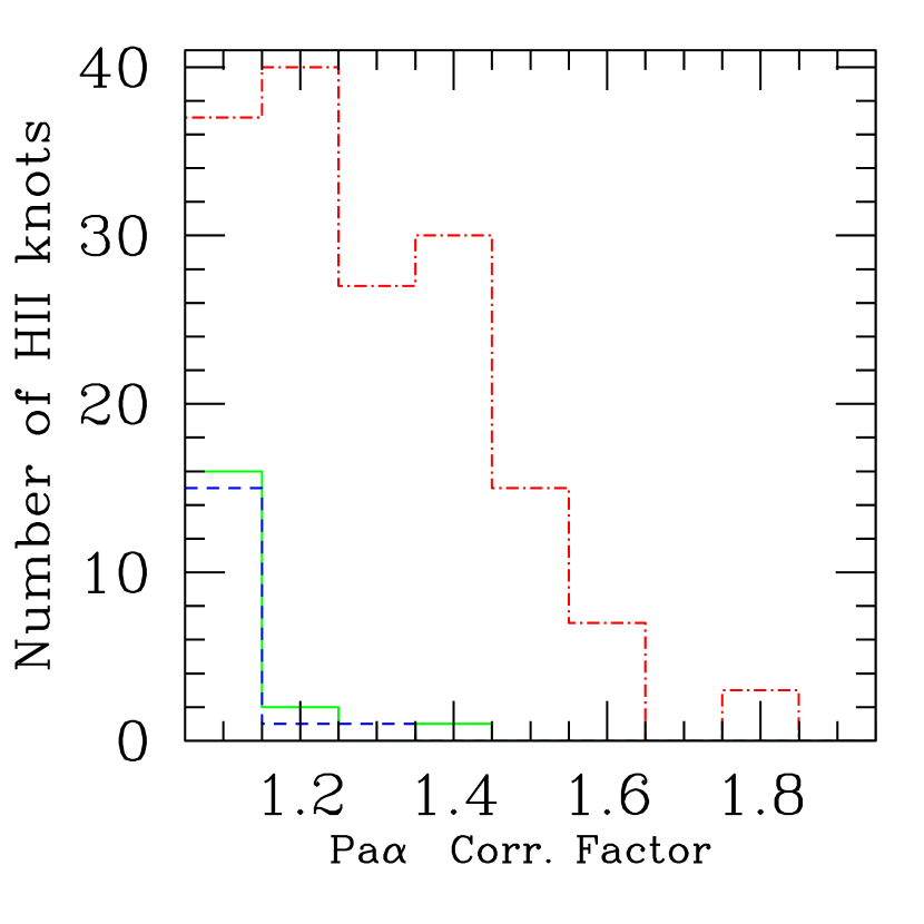
Figure 2: Histogram of the multiplicative factors applied to the observed Pa$\alpha$ line emission to correct for the effects of dust extinction, as determined using the H$\alpha$/Pa$\alpha$ ratio (section 3.2). The vertical axis shows the number of HII knots to which each correction factor is applied. The high (12$+$log(O/H)$>$8.35), medium (8.00$<$12$+$log(O/H)$\lesssim$8.35), and low (12$+$log(O/H)$\lesssim$8.00) metallicity regions (section 2) are shown as three separate histograms, coded as red dot–dash line, green continuous line, and blue dash line, respectively. Most corrections are less than 50%.

The HST/NICMOS observations are the shallowest in our sample when compared to the other images, and represent the true limitation to our analysis. On the other hand, Pa$\alpha$ measurements offer an opportunity to obtain a nearly unbiased measure of the number of ionizing photons produced in a region, as it is only weakly affected by dust extinction. An extinction as large as 5 mag at V produces an extinction of 0.73 magnitudes at Pa$\alpha$, i.e., roughly a change of a factor of 2 in the line intensity (Figure 2), for foreground screen dust geometry. Still, we combine the Pa$\alpha$ measurements with complementary measurements at H$\alpha$ to correct the line emission for the effects of dust. We adopt a metallicity–dependent intrinsic ratio H$\alpha$/Pa$\alpha$=7.82, 8.45, and 8.73 for the high, medium, and low metallicity subsamples, respectively, which correspond to electron temperatures T_e=7,000 K, 10,000 K, and 12,500 K for the HII knots (for n_e=100 cm^-3 Osterbrock & Ferland, 2006; Garnett, Kennicutt & Bresolin, 2004). We also adopt an extinction curve with differential value k(H$\alpha$)$-$k(Pa$\alpha$)=2.08 (Fitzpatrick, 1986; Landini et al., 1984).

Four of the galaxies discarded from our sample (Table 1) present an array of problems mainly in their NICMOS observations. The F187N image of NGC0024 is heavily affected by cosmic ray persistence, which has caused the effective noise level of the frame to be about 7 times higher than nominal; the net result is that the faint emission from the galaxy is undetectable. The NICMOS frames of NGC1291 missed the galaxy because of guide star problems. The F187N images of NGC4631 show a faint flat–field imprint (generally a sign of residual pedestal) that, coupled with the large dynamical range of the emission from this edge–on galaxy, produces a very uneven background. For NGC3034 (M82) , problems related to non-linearity corrections and saturation for this bright target exist for the NICMOS, IRAC, and MIPS images, making photometry in the center of this object highly unreliable at the present time.

The HST archive was also mined for H$\alpha$ images for those cases where (a) coverage was similar between NIC3 and optical images, and (b) the narrowband filter provides a better rejection of the [NII] emission line than the ground–based images. WFPC2 images that met these criteria were available for NGC1512, NGC4736, NGC4826, and NGC5055. The line emission was observed through the narrowband filters F656N or F658N, and the underlying continuum through F547M, F555W, and/or F814W (equivalent to medium–V, V, and I, respectively). For NGC4736, NGC4826, and NGC5055, the [NII]/H$\alpha$ values listed in Table 2 come from the comparison of the fluxes in the HST and ground–based (see below) narrowband filters; the [NII] contamination in the HST filters is minimal, and has been used to guide our extrapolation of the best nitrogen–to–H$\alpha$ ratio to attribute to each galaxy. This value has been used for those areas in the ground–based images not covered by the HST.

3.3 Ground–based Optical Imaging Data

R–band and H$\alpha$–centered narrowband images were obtained for most of the galaxies as part of the SINGS ancillary data program, either at the 2.1–m KPNO telescope or at the 1.5–m CTIO telescope (Kennicutt et al., 2003). Exposure times were typically around 1800 s for the narrowband filters, and a few hundred seconds for R. Standard reduction procedures were applied to all the images. Standard stars observations were obtained during each observing run to derive photometric calibrations.

The rescaled broadband images were subtracted from the narrowband images to obtain emission–line–only images. The [NII] contamination within the filter bandpass is removed using [NII]/H$\alpha$ values measured either from large–aperture ($\approx$50^′′) SINGS optical spectroscopy (Moustakas et al., 2007) or retrieved from the literature (Table 2), and accounting for changes in the filter transmission between the wavelengths of H$\alpha$ and the two [NII] emission lines. High metallicity galaxies for which [NII]/H$\alpha$ ratios are not available from either source, or cases which have optical spectra dominated by a central non–thermal source (Seyfert 2 or LINER, Moustakas et al., 2007) are assumed to have [NII]/H$\alpha\sim$0.5. Within each galaxy, a constant [NII]/H$\alpha$ is adopted, although the ratio can change significantly from individual HII regions to the more diffuse component (Hoopes & Walterbos, 2003). Radial variations of [NII]/H$\alpha$ within a galaxy are less of a concern here, as only the central region of each galaxy is imaged.

Typical 1 $\sigma$ sensitivity limits of the final H$\alpha$ images are 1–2$\times$10^-17 erg s^-1 cm^-2 arcsec^-2, i.e., they are a factor 3–10 deeper than the Pa$\alpha$ images. This, coupled with the fact that the H$\alpha$ is, intrinsically, about 8 times brighter than Pa$\alpha$, implies that our H$\alpha$ measurements will have higher signal–to–noise ratio than the Pa$\alpha$ ones for A${}_{V}\lesssim$4 mag.

Narrowband and R–band images of DDO053, M81DwB, Holmberg9, and NGC4625 were obtained using a CCD imager on the Steward Observatory Bok 2.3 m telescope, as part of the 11HUGS project (Kennicutt et al., 2007b). Narrowband and R–band images of NGC5408 were obtained at the CTIO 0.9–m telescope, also as part of the 11HUGS project. Images were taken using a 70 Å narrowband filter centered at 6580 Å and an R-band filter and a Loral 2kx2k CCD detector. Exposure times were 1000 s in H$\alpha$ and 200 s in R, and reach comparable depth to the KPNO images because of the high throughputs of the filter and the CCD detector. Data reduction followed similar procedures as described above.

Ground–based H$\alpha$ images for NGC3627, NGC4736, NGC4826, and NGC5055 were provided by the SONG collaboration (Sheth et al., 2002; Helfer et al., 2003), as SINGS did not repeat these observations. The data were obtained at the KPNO 0.9–m telescope, with an observing strategy and filter selection similar to those of SINGS. The main difference between the SINGS and SONG H$\alpha$ images is the total exposure time (and the depth of the images), being in the latter case 3–5 times shorter than in the former. For this reason, the ground–based SONG images were used in conjunction with the HST H$\alpha$ images for photometric measurements in NGC4736, NGC4826, and NGC5055.

4 Photometric Measurements

4.1 Aperture Photometry

For each galaxy, the H$\alpha$, stellar–continuum–subtracted 8 $\mu$m, and 24 $\mu$m images were registered to the same coordinate system of the Pa$\alpha$ image, before performing measurements. Photometric measurements at all four wavelengths of local 24 $\mu$m and H$\alpha$ peaks were performed on the common field of view of the four images. Emission peaks at 24 $\mu$m (and 8 $\mu$m) have generally corresponding H$\alpha$ peaks; the opposite, however, is not always true, and there are some cases of H$\alpha$ emission peaks without corresponding mid–IR emission. Thus, both 24 $\mu$m and H$\alpha$ images were used independently to locate local peaks of star formation.

The size of the aperture used for photometric measurements is dictated by the lowest angular resolution image, the MIPS 24 $\mu$m image, with a PSF FWHM$\sim$6^′′. We chose apertures with 13^′′ diameter as a compromise between the desire to sample the smallest possible scale compatible with HII regions and the necessity to have reasonable aperture corrections on the photometry (Figure 1). For the chosen aperture size, corrections to infinite aperture are 1.045, 1.05, and 1.67 at 3.6 $\mu$m, 8 $\mu$m, and 24 $\mu$m, respectively, for point sources (SSC IRAC Handbook and MIPS Handbook, respectively; Reach et al., 2005; Engelbracht et al., 2007; Jarrett, 2006), and are assumed to be small or negligible in the Pa$\alpha$ and H$\alpha$ images (Calzetti et al., 2005).

In the case of the IRAC 3.6 $\mu$m and 8 $\mu$m emission, extended emission has a different aperture correction than point sources. Best current estimates (Jarrett, 2006) indicate that our aperture choice requires an additional correction factor 1.02 at 3.6 $\mu$m and 0.90 at 8 $\mu$m, for extended sources. As our sources are neither totally extended nor point–like, actual aperture corrections are likely to be closer to a value of unity than those reported here.

The fixed aperture corresponds to different spatial scales in different galaxies, as distances between $\sim$0.5 Mpc (spatial scale $\sim$30 pc) and $\sim$20 Mpc ($\sim$1.26 kpc) are covered. In order to allow comparison among luminosities measured over areas that differ by a factor as much as $\sim$40 (for the typical distance range 3–20 Mpc), we report all measurements as luminosities per unit of physical area (luminosity surface density, LSD) S_Paα, S_Hα, S${}_{8\mu m,\ dust}$, and S_24μm, in units of erg s^-1 kpc^-2. Luminosities at mid–infrared wavelengths are expressed as $\nu$L($\nu$).

The use of luminosity surface densities removes most dependence of our measurements with distance, as the LSDs are, for our purposes, equivalent to fluxes. Notable exceptions are the cases where the area covered by our aperture contains only one HII region, with intrinsic size smaller than our adopted fixed aperture’s size; in these cases the LSDs will be artificially decreased by the larger area of the aperture relative to the values they would have if we selected apertures matched to the intrinsic size of each HII region/complex. The latter choice is not easily applicable to our sample due to the angular resolution limitations of some of the data. Furthermore, we will see in section 6 that this effect does not appear to have an important impact on our results.

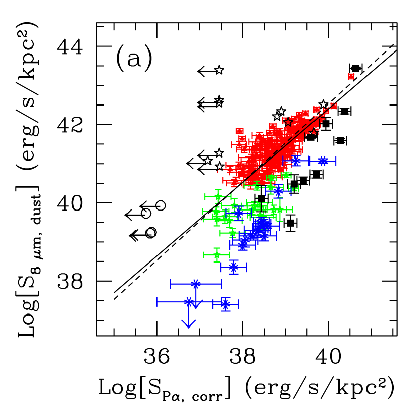
Figure 3: (a) Luminosity surface density at 8 $\mu$m, S${}_{8~{}\mu m,\ dust}$, as a function of the extinction–corrected LSD at Pa$\alpha$, S_Paα,corr, for the 220 HII knots in the 33 galaxies for which photometric measurements have been obtained. LSDs are averaged over 13^′′ photometric apertures. The 8 $\mu$m emission is stellar continuum–subtracted (section 3.1). Data points are divided into three metallicity bins: high (red filled triangles), medium (green stars), and low (blue asterisks) oxygen abundance (section 2). Filled black squares mark the local starbursts from the sample of Engelbracht et al. (2005) (section 5.1). 3 $\sigma$ error bars are indicated for each data point. Open black star symbols indicate the location of the non-thermal sources (Sy2s or LINERs, section 4.1) and open black circles indicate extended background sources. The best fit line through the high metallicity (red) datapoints is shown as a continuous line, while the dashed line is the linear fit through the same datapoints with fixed slope of 1. (b) Histogram of the deviation of the HII knot data in panel (a) from the best fit line through the high metallicity data (the continuous line in panel (a)). The values of the best–fit coefficients are c=(0.94$\pm$0.02) and d=(4.80$\pm$0.85) (equation 2). Three separate histograms are shown, for high (red), medium (green), and low (blue) metallicity data. The medium and low metallicity histograms have been multiplied by a factor 2 to make them visible.

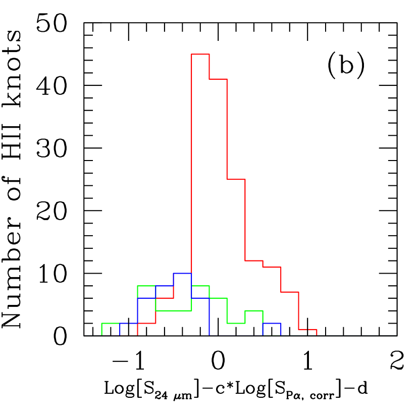
Figure 4: (a) and (b). The same as Figure 3, for the luminosity surface density at 24 $\mu$m, S${}_{24~{}\mu m}$. In addition to the same datapoints as Figure 3, panel (a) also reports the Luminous InfraRed Galaxies (LIRGs) from the sample of Alonso–Herrero et al. (2006) (black asterisks; section 5.2). The values of the parameters (c, d) in the horizontal axis of of panel (b), are given in equation 3, and are c=(1.23$\pm$0.03) and d=($-$6.88$\pm$0.97).

Photometry for a total of 220 separate HII knots is obtained in the 33 galaxies. Of these, 179 are in the 23 high metallicity galaxies, including 11 non–thermal nuclei (Seyfert 2 or LINERs as retrieved from NED; no aperture was laid on top of the active nucleus of the edge–on galaxy NGC5866). In the five medium metallicity and five low metallicity galaxies, 22 and 19 regions are measured, respectively, including 4 regions (one each in IC2574, Holmberg IX, M81DwB, and NGC6822) that are strongly emitting in the mid-infrared, but are undetected in both our Pa$\alpha$ and H$\alpha$ data. These line–undetected objects are detected in the optical continuum bands and are extended; thus they are likely background sources. Heavily obscured sources, like those discussed in Prescott et al. (2007), should represent about 3% of the 24 $\mu$m sources, but we find none; we attribute this lack of heavily obscured sources in our sample to the small spatial region subtended by the NICMOS FOV within each galaxy. The 11 non–thermal sources and the 4 background sources (Figures 3–4) will be excluded from all subsequent statistical analysis.

Crowding of emission peaks within each frame prevents the use of ‘annuli’ around individual apertures to perform background subtraction from the photometric measurements. Background removal is thus achieved by subtracting a mode from each frame, as described in Calzetti et al. (2005).

‘Integrated’ values of H$\alpha$, Pa$\alpha$, 8 $\mu$m, and 24 $\mu$m luminosity surface density are also derived for each galaxy within the area imaged by the NICMOS/NIC3 camera. These integrated values are therefore the LSD of each galaxy within the central $\sim$50^′′, except for NGC5194, where the central $\sim$144^′′ are measured (Table 2). The integrated values mix the emission from the star forming regions (measured with the smaller apertures) with areas of little or no star formation, thus providing some insights into the impact of the complex galactic environment on SFR calibrations.

4.2 Uncertainties in the Photometric Measurements

The uncertainties assigned to the photometric values at each wavelength and for each galaxy are the quadrature combination of four contributions: Poisson noise, variance of the background, photometric calibration uncertainties, and variations from potential mis-registration of the multiwavelength images. The variance on the image background is derived in each case from the original–pixel–size images. The impact of potential background under– or over–subtractions varies from galaxy to galaxy, and also depends on the relative brightness of the background and the sources. The effect of potential misregistrations have been evaluated for the case of NGC5194 by Calzetti et al. (2005). Because of the large apertures employed for our photometry, this contribution is either small (a few %  of the total uncertainty) or negligible.

For the Spitzer 8 $\mu$m and 24 $\mu$m images, calibration uncertainties are around 3% and 4%, respectively (Reach et al., 2005; Engelbracht et al., 2007). This, added in quadrature to the other uncertainties, produces overall uncertainties in the measurements that range between 15% and a factor of two, with the median value being around 22%. The superposition of the PSF wings in adjacent apertures produces an additional effect in the 24 $\mu$m measurements, that is evaluated and removed on a case–by–case basis (see example in Calzetti et al., 2005).

For the HST images, photometric calibrations are generally accurate to within $\sim$5%, for narrowband filters. The faintness of the Pa$\alpha$ emission, and therefore the impact of the background variance and stellar continuum subtraction is what mostly dominates the photometric uncertainty on the Pa$\alpha$ emission line measurements, with values between 15% and a factor of roughly 2, with a median value of 60%. For the extinction–corrected Pa$\alpha$ luminosities, the uncertainty on the attenuation A_V increases the Pa$\alpha$ uncertainty by a factor of 1.22.

For the ground–based H$\alpha$ images, which are the deepest images in our set, the main sources of uncertainty are: photometric calibrations, stellar continuum subtraction, and the correction for the [NII] contribution to the flux in the narrow–band filter. These translate into uncertainties in the final photometric values between 10% and 50% (with occasional factor–of–2 uncertainty). The median uncertainty for the H$\alpha$ luminosities is 20%. Although less deep, the HST H$\alpha$ images are characterized by more stable photometry, better continuum subtraction, and smaller [NII] contamination; uncertainties on the final luminosities are in the range 5%–10%.

For a few of the galaxies of Table 2, some special circumstances are present or special treatment was required. For NGC2841, the very faint line emission produces large, and highly uncertain, A_V values. For NGC5033, no H$\alpha$ image is available; the uncorrected Pa$\alpha$ can be up to 70% underestimated for the largest A_V measured in our sample (A${}_{V}\sim$4 mag), and, therefore, this galaxy is excluded from all fits reported below.

In Holmberg IX, H$\alpha$ emission is detected in two of the three selected regions; for one of these two regions, 24 $\mu$m emission is also detected, at the $\sim$2.5 $\sigma$ level. A strong 24 $\mu$m detection is present in the third region, together with the only 8 $\mu$m detection in the field; because of the absence of hydrogen line emission and of the extended nature of the broad band emission, this source is identified with one of the background sources discussed in section 4.1. For the two regions with H$\alpha$ emission, only upper limits can be derived for the Pa$\alpha$ and 8 $\mu$m emission. The presence of H$\alpha$ emission provides a lower limit to the Pa$\alpha$ line intensity for the zero extinction case (after including the uncertainty on the H$\alpha$ measurement itself). We have taken the range between this lower limit and the upper limit measured from the HST/NICMOS images to be our fiducial range of values for Pa$\alpha$, and therefore we report the middle values (in logarithmic scale) as measurements, rather than use the actual upper limits.

In NGC5408, the brightest, and most extended, line–emitting region is only partially imaged by NICMOS. The Pa$\alpha$ image is therefore used only to derive a typical A_V value for the region, using small-aperture photometry and the matching H$\alpha$ measurements. The A_V value derived in this way is then applied to the H$\alpha$ emission of the entire, extended, region, for which a larger–than–nominal, 17.1^′′ diameter, aperture is used, not only for H$\alpha$, but also for the 8 $\mu$m and 24 $\mu$m emission. The other two regions in this galaxy are treated with the nominal procedure described in section 4.1.

5 Starburst Galaxies

Our baseline sample of 220 HII knots is augmented with 10 local low–metallicity starburst galaxies and 24 LIRGs from Engelbracht et al. (2005) and Alonso–Herrero et al. (2006), respectively, in order to verify that trends and correlations observed for star–forming regions within galaxies can also be applied to galactic–scale ($\sim$kpc) star formation. In this context, starbursts are defined as galaxies with a central, connected star forming region whose energy dominates the light output in the wavebands of interest.

The low–metallicity starbursts and the LIRGs also expand the mid–IR and line emission LSD parameter space of the low– and high–metallicity HII knots, respectively, by more than an order of magnitude at the high end.

5.1 Low–Metallicity Starburst Galaxies

As part of the HST/NICMOS SNAP–9360, about 40 nearby starburst galaxies were observed. Of these, 13 also have Spitzer imaging as part of the MIPS and IRS GTO observations (Engelbracht et al., 2005). The main characteristics and measurements for 10 of these galaxies are listed in Tables 3 and 4. The three remaining galaxies, NGC3079, NGC3628, and NGC4861, are omitted from the present analysis for the following reasons. For NGC4861, the HST/NICMOS pointing targeted the relatively quiescent center of this galaxy, rather than the peripheral giant HII region. The other two galaxies, NGC3079 and NGC3628, have extended optical line and mid–IR emission: about 40% and 60% of the emission is outside of the field–of–view imaged by HST/NICMOS; corrections for the fraction of light in the Pa$\alpha$ line outside of the observed frame would be thus substantially larger than the typical uncertainties in the measurements.

The data for the galaxies in Table 3 were reduced in the same fashion as the SINGS galaxies discussed in sections 2–3. In particular, the HST/NICMOS images, which are presented here for the first time, were treated following the same procedure as section 3.2. The main difference between the HII knots in the SINGS galaxies and the local starbursts is in the photometry: integrated flux values encompassing the entire central starburst (the dominant source of emission at the wavelengths of interest) are derived for the latter sample. The integrated measurements at 8 $\mu$m and 24 $\mu$m are from Engelbracht et al. (2005), and are reported in Table 4.

The Pa$\alpha$ measurements (Table 4) are performed using the aperture sizes listed in Table 3, and are corrected for the Galactic foreground extinction (fourth column of Table 3), but not for internal extinction. We expect the internal extinction to represent a small effect on the Pa$\alpha$ flux in these mostly low metallicity galaxies (compare with Figure 2). An exception may be represented by SBS0335-052, for which Houck et al. (2004) measure A${}_{9.7~{}\mu m}\sim$0.5 mag. If the region of silicate absorption is coincident with the region of line emission, this would correspond to A${}_{Pa\alpha}\sim$2 mag. Given the uncertainty in the spatial co-location of the dust-hidden source detected by Houck et al. (2004) and the main source(s) of the Pa$\alpha$ emission and the fact that the introduction of an extinction correction for one of the galaxies does not impact our conclusions, we do not perform the correction.

5.2 Luminous Infrared Galaxies

HST/NICMOS Pa$\alpha$ data and extinction corrections, as well as information on the physical extent of the star forming area for each of the 24 LIRGs used in this analysis, are presented in Alonso–Herrero et al. (2006); the reader is referred to that work for details. Infrared measurements at 25 $\mu$m from IRAS and distances for each galaxy are from Sanders et al. (2003) and Surace, Sanders & Mazzarella (2004). At the time of this writing, no 8 $\mu$m emission measurements are available for these galaxies. The LIRGs’ metallicities are characteristic of our high–metallicity HII knots sample (Alonso–Herrero et al., 2006). Photometry for these galaxies, as in the case of the local starbursts (section 5.1), includes the entire line–emitting and IR–emitting galactic region, thus the measurements are integrated galaxy values.

6 Analysis and Results

Photometric measurements for the 220 HII knots, the local low–metallicity starbursts, and the LIRGs are shown in Figures 3–4, where the infrared LSD in the two mid–IR wavebands is shown as a function of the extinction–corrected Pa$\alpha$ LSD.

One characteristic immediately apparent in Figures 3–4 is the overall correlation between the infrared LSDs and the Pa$\alpha$ LSD (panels [a]), although the scatter is non negligible in both cases (panels [b]). The correlations appear especially significant for the high metallicity HII knots (the most numerous subsample among those under analysis here), and span a little over two orders of magnitude in Pa$\alpha$ LSD. Bi-linear least–square fits through the high–metallicity data points yield:

$$Log\ S_{8~{}\mu m,\ dust}=(0.94\pm 0.02)\ Log\ S_{Pa\alpha,corr}+(4.80\pm 0.85),$$ (2)

$$Log\ S_{24~{}\mu m}=(1.23\pm 0.03)\ Log\ S_{Pa\alpha,corr}-(6.88\pm 0.97),$$ (3)

where S_Paα,corr is the extinction–corrected Pa$\alpha$ LSD. Equation 3 accounts effectively for the trend of the LIRGs, although these data were not used in the fitting procedure.

The scatter of the datapoints about the best fit lines of equations 2–3 are approximately the same, with $\sigma$=0.3 dex (panels (b) of Figure 3–4). Thus the 1 $\sigma$ scatter is about a factor of 2 for the high metallicity regions.

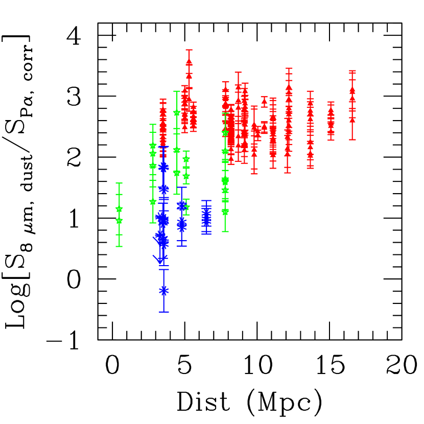
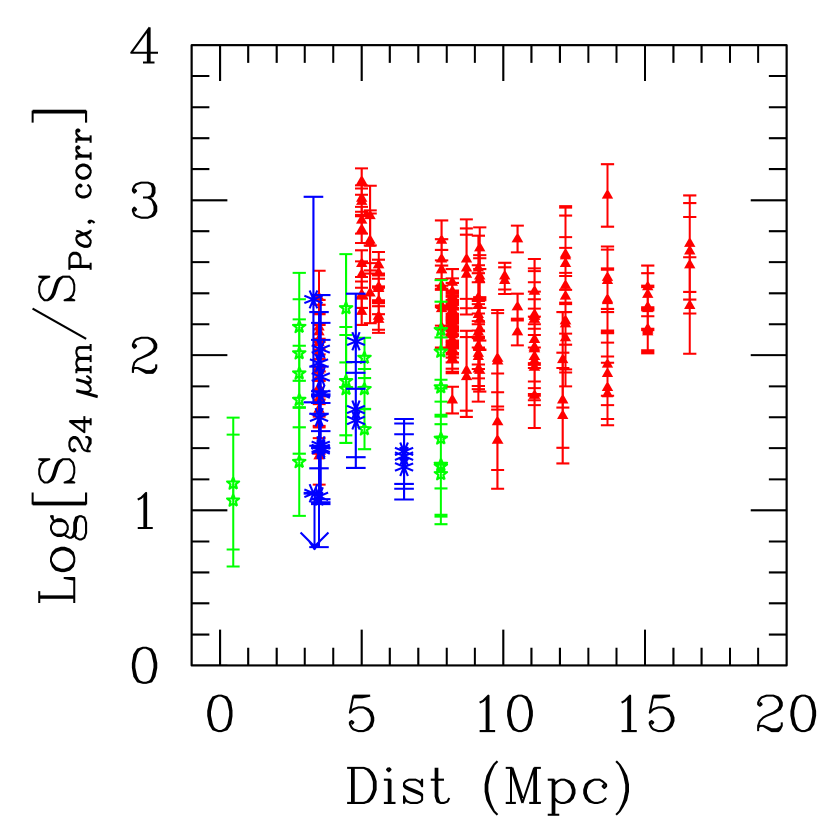
Figure 5: The ratio of the mid–IR to the extinction–corrected Pa$\alpha$ LSDs, as a function of the galaxies’ distances, for the 8 $\mu$m (left) and the 24 $\mu$m (right) HII knot measurements, respectively. Background sources and non–thermal sources are not included. In both panels, the high–metallicity datapoints are consistent with no correlation of the ratio as a function of distance, implying that the correlations between the mid–IR emission and the Pa$\alpha$ emission are not driven by distance effects. The 8 $\mu$m emission of the medium and low–metallicity HII knots remains on average deficient relative to that of the high–metallicity data also when only galaxies at similar distances are considered (thus flux measurements are performed in similar–size regions). With the possible exception of NGC 6822, which is at a distance of only 0.47 Mpc and shows lower–than–average values for its metallicity bin, the observed 8 $\mu$m emission deficiency in metal–poor regions is not an effect of a bias in the size of the regions that are being measured.

A potential source of bias in equations 2 and 3 is the large range of distances that our sample covers, about a factor of 6 for the high metallicity galaxies. Our fixed photometric aperture of 13^′′ diameter thus probes regions that are about 30 times different in area between the nearest and the farthest targets in the high metallicity subsample, i.e., from 0.04 kpc² at 3.5 Mpc to 1.12 kpc² at 17 Mpc (for the most distant galaxy in our sample, NGC4125, located at 21 Mpc, only the central Sy2 nucleus is detected and is excluded from the analysis). Although we remove the background from each photometric measurement, uncertainties in this subtraction will affect the farthest targets more strongly than the closest ones, if HII regions/complexes have constant sizes of $\approx$100–200 pc. Furthermore, we may expect that our fixed aperture photometry may dilute the LSDs of the more distant regions, for the extreme hypothesis that only one HII region is contained in each aperture. We have tested the impact of these effects by looking at the distribution of the ratios S${}_{8~{}\mu m,\ dust}$/S_Paα,corr and S${}_{24~{}\mu m}$/S_Paα,corr as a function of galaxy distance (Figure 5). For the high metallicity subsample, non–parametric (both Spearman and Kendall) tests show that the data are uncorrelated with the galaxy’s distance, suggesting that there is no obvious bias in our analysis.

Both the 8 $\mu$m and 24 $\mu$m LSDs of medium and low metallicity regions are deficient relative to the extrapolation of the best fit lines for the high metallicity regions (Figure 3 and 4). The deficiency is far more pronounced in the case of S${}_{8\mu m,\ dust}$, a fact already noted in a number of previous investigations (e.g., Engelbracht et al., 2005; Galliano et al., 2005; Hogg et al., 2005; Rosenberg et al., 2006; Draine et al., 2007). A potential source of concern in this case is that the high metallicity subsample has a higher mean distance than the medium and low metallicity ones (Figure 5). Helou et al. (2004) have shown that the 8 $\mu$m emission is brighter at the edges of an HII region (i.e., in the PDR) than at its center. Our fixed aperture photometry could therefore underestimate the 8 $\mu$m flux from the low metallicity regions, if the apertures are not large enough to sample the entire area surrounding the HII knot. However, Figure 5 shows that the 8 $\mu$m emission is deficient in the medium and low metallicity subsamples relative to the high metallicity one even when galaxies at comparable distances are considered. The only potential exception is NGC 6822, the closest galaxy to the Milky Way in our sample, which, at a distance of 0.47 Mpc, could suffer from the effect of having too a small aperture applied to the 8 $\mu$m emission measurements; indeed its mean value is lower (although not statistically significantly) than the average of the other data in the same metallicity bin.

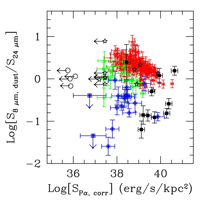
Figure 6: Ratio of the 8 $\mu$m to 24 $\mu$m LSD as a function of the extinction–corrected Pa$\alpha$ LSD for the 220 HII knots and for the local starbursts. Symbols and colors are as in Figure 3. The deficiency of the 8 $\mu$m emission, relative to the 24 $\mu$m emission for the low–metallicity datapoints is independent of the average ionizing photon rate in the region. The decrease of the 8 $\mu$m to 24 $\mu$m LSD ratio as a function of increasing Pa$\alpha$ LSD for the high metallicity points indicates that the component of thermal equilibrium dust contributing to the 24 $\mu$m emission is increasing in strength (the dust is in thermal equilibrium and ‘warmer’ at higher ionizing photon densities, see, Helou, 1986; Draine & Li, 2006). A contribution to the decrease of the 8 $\mu$m emission due to increased destruction rate of the carriers for increasing starlight intensity (Pa$\alpha$ LSD) may also be present (Boulanger et al., 1988).

The trend of the S${}_{8\mu m,\ dust}$/S_24μm ratio as a function of S_Paα,corr (Figure 6) highlights the decrease of the 8 $\mu$m LSD for decreasing metallicity, and also shows that the effect is independent of the number of ionizing photons in the region. The latter suggests that: (1) our aperture sizes are large enough to encompass both the HII regions and the surrounding PDRs, as noted above; and (2) in these large regions the dependence of the 8 $\mu$m–to–24 $\mu$m ratio on the luminosity surface density of the HII region/complex that heats the dust is a small effect relative to the effect of metallicity. The decrease of the 8 $\mu$m to 24 $\mu$m LSD ratio as a function of increasing Pa$\alpha$ LSD in the high metallicity points (i.e., at roughly constant metallicity) indicates that the component of thermal equilibrium dust contributing to the 24 $\mu$m emission is increasing in strength (the dust is in thermal equilibrium and ‘warmer’ at higher ionizing photon densities, see Helou, 1986; Draine & Li, 2006). An additional contribution may also come from an increased destruction rate of the 8 $\mu$m dust emission for increasing starlight intensity (Boulanger et al., 1988).

As suggested by Kennicutt et al. (2007a), the combination of measurements at H$\alpha$ and 24 $\mu$m can provide insights into both the unobscured and obscured regions of star formation. We have combined linearly the observed H$\alpha$ and 24 $\mu$m LSDs and scaled them to the Pa$\alpha$ LSD. The best fit line through the data is:

$$Log\ S_{Pa\alpha,corr}=(0.98\pm 0.02)\ Log\ (aS_{H\alpha,obs}+bS_{24~{}\mu m})+(0.73\pm 0.93)$$ (4)

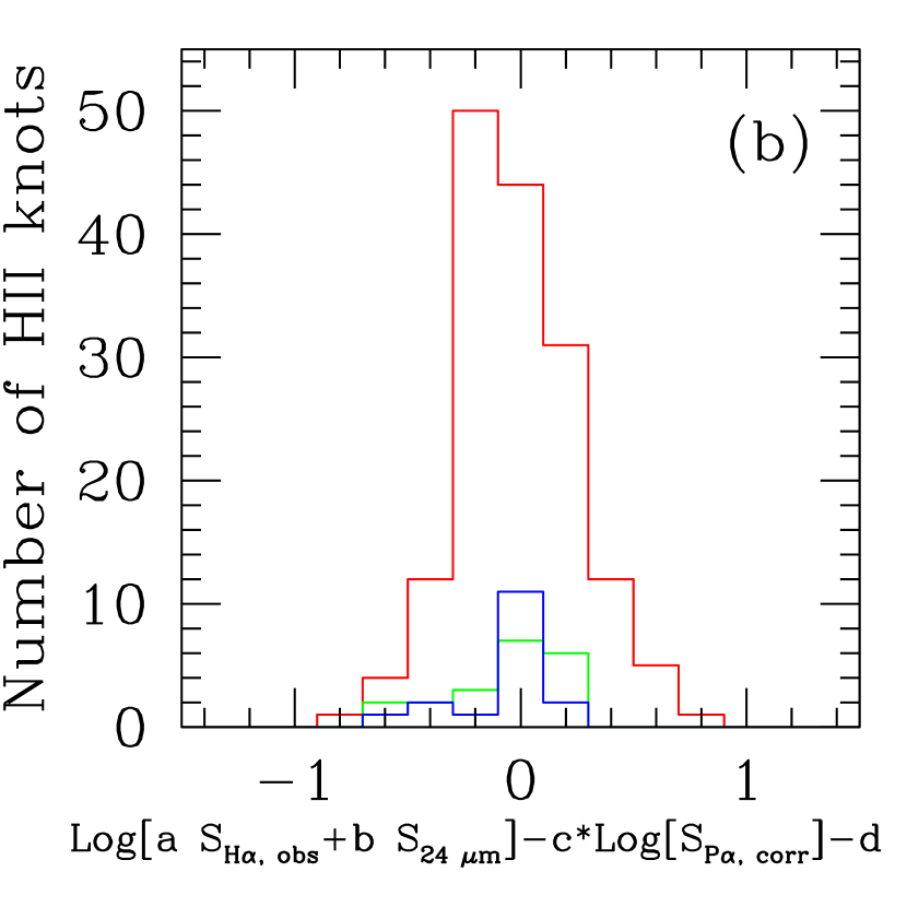
Figure 7: (a) and (b). As Figure 4, for the linear combination of H$\alpha_{obs}$ and 24 $\mu$m LSD (equation 4). Symbols are as in Figures 3 and 4. (Panel a): Data for the HII knots and the LIRGs. The best fit line through the high metallicity HII knots (continuous line) is not significantly different from a linear relation with slope of unity (dashed line). (Panel b): Histogram of the deviation of the HII knot data in panel (a) from the best fit line through the high metallicity data (the continuous line in panel (a)). Unlike Figures 3 and 4, the histograms of the medium and low metallicity datapoints have not been multiplied by a factor 2. The values of the x–label parameters (c, d) are derived from equation 4 and are c=(1.02$\pm$0.02) and d=($-$0.74$\pm$0.97).

where $a$ is the intrinsic Pa$\alpha$/H$\alpha$ ratio, thus is dictated by atomic physics and is only moderately dependent on metallicity ($a$=0.128, 0.118, and 0.114 for the high, medium, and low metallicity data, respectively; see section 3.2). The coefficient $b$ for the 24 $\mu$m LSD has been empirically rescaled to bring the sum of the optical and IR LSDs in agreement with the Pa$\alpha$ one ($b$=0.0040, 0.0037, and 0.0036 for the high, medium, and low metallicity datapoints, respectively; Figure 7). The best fit from equation 4 gives $b/a$=0.031$\pm$0.006, and this ratio is independent of metallicity. Equation 4 is, within the uncertainties, consistent with a linear relation with null intercept between the two quantities, as expected if the right–hand–side expression is a measure of the ionizing photon rate, like S_Paα,corr. The linearity of the relation is by construction, as the requirement is to approach unity as much as possible for all the combined data, but the null intercept has not been fixed a priori; furthermore, the ratio b/a was left as a free parameter in the analysis, and its constant value is a result (not an input).

Interestingly, the high metallicity datapoints show approximately the same dispersion around the mean trend of equation 4 as they do for equations 2 and 3, with a 1 $\sigma\sim$0.3 dex. In the case of the combined optical/mid–IR, the dispersion is the same whether the high metallicity datapoints alone or all datapoints are included in the statistical analysis (panel (b) of Figure 7). Conversely, for the two mid–IR LSDs the dispersion is measured for the high metallicity datapoints only, and increases substantially (on one side) when the medium and low metallicity datapoints are included in the statistics (panels (b) of Figures 3 and 4). These considerations do not include the LIRGs, that in Figure 7 show evidence of having higher combined optical/mid–IR LSDs than inferred from the extrapolation of equation 4. A possible explanation for this effect will be discussed in Section 7.

As already discussed in Kennicutt et al. (2007a), the sum on the right–hand–side of equation 4 can be interpreted as a representation of the dust extinction corrected H$\alpha$ luminosity or LSD. as:

$$S_{H\alpha,corr}=S_{H\alpha,obs}+(0.031\pm 0.006)S_{24~{}\mu m}.$$ (5)

The proportionality coefficient for the 24 $\mu$m luminosity is $\sim$20% smaller than that derived for NGC5194 alone (Kennicutt et al., 2007a), which is within the 1 $\sigma$ uncertainty. This small difference is likely due to the larger variety of galaxies used in the present work which provides a dynamical range in luminosity surface density about an order of magnitude larger than in the NGC5194 case.

The proportionality coefficient for the 24 $\mu$m emission in equations 4 and 5, b/a=0.031, is independent of metallicity. This suggests that in the S_24μm versus S_Paα,corr plane the observed deviations of the medium and low metallicity data from the best fit for the high–metallicity datapoints are simply due to the progressively lower dust content of the ISM for decreasing metallicity (section 7). No other effect beyond the simple increase in the medium’s transparency is required. Indeed, most of the contribution to S_Hα,corr comes from the observed H$\alpha$ emission at low S_Paα,corr LSDs (low dust systems) and, vice-versa, it is mainly contributed by the 24 $\mu$m emission at the high LSD end of our sample (dusty systems).

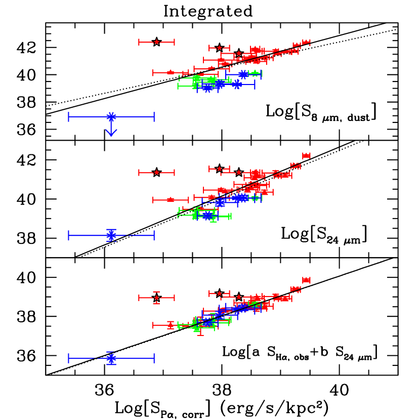
Figure 8: Mid–IR or combined–optical/mid–IR LSD as a function of the extinction–corrected Pa$\alpha$ LSD, averaged over the entire central region covered by the HST/NICMOS observations, for each of the star–forming galaxies from Table 1 (section 4.1). The three panels show on the vertical axis, from top to bottom, the 8 $\mu$m, 24 $\mu$m, and the linear combination of H$\alpha$ and 24 $\mu$m LSDs in logarithmic scale, as indicated by the label at the bottom–right corner of each plot; the vertical axis has the same units as the horizontal axis, erg s^-1 kpc^-2. Each HST/NICMOS image is about 50^′′ in size, except for NGC5194, where a region of 144^′′ in size has been observed. Color coding of each galaxy is the same as the HII knots in Figure 3. The continuous lines are the best linear fit through the high metallicity (red triangles) data, after excluding the Sy2–dominated fluxes of NGC4569, NGC4736, and NGC5195 (marked as black stars), thus leaving 19 independent datapoints. The dotted lines are the best fits through the high metallicity HII knots from Figures 3, 4, and 7 for S${}_{8\mu m,\ dust}$, S_24μm, and a S${}_{H\alpha,obs}+$b S_24μm, respectively.

Similar correlations as those seen for the HII knots within galaxies exist between the integrated LSDs of the galaxies’ centers (section 4.1). Figure 8 shows the trends for the 33 star–forming galaxies in our main sample. For the combined optical/mid–IR LSDs, a linear fit through the integrated datapoints of the high metallicity galaxies are consistent, within 1 $\sigma$, with the best fit lines through the individual HII knots, both in slope and intercept (third panel of Figure 8). For the 24 $\mu$m LSD, the slope of the linear fit is consistent (again within 1 $\sigma$) with that of the individual HII knots, and the intercept is consistent (within 0.1 $\sigma$) with the value expected by simply rescaling the HII knots’ mean LSD for the larger area used in the integrated measures. The results for both the 24 $\mu$m and the combined optical/mid–IR integrated measures suggest that within the central areas covered by the NICMOS observations any diffuse 24 $\mu$m emission contributing to the measured LSD is matched by diffuse Pa$\alpha$ LSD with comparable intensity. This, of course, does not mean that diffuse 24 $\mu$m emission is not present; indeed, such diffuse emission has been observed in the SINGS galaxies (Dale et al., 2006). Our result simply implies that such diffuse 24 $\mu$m emission traces the diffuse ionized emission, at least within the central galaxy regions sampled by our data.

A more complicated scenario appears for the 8 $\mu$m LSD: a best fit line through the high metallicity integrated regions produces a higher slope (1.16$\pm$0.09) than derived for the individual HII knots. The difference is marginally significant (2.2 $\sigma$), but implies that the 8 $\mu$m LSD is higher by about a factor of 2 over what is expected from a simple rescaling of areas at the high luminosity end. A visual inspection of the images shows that the galaxies with low 8 $\mu$m LSDs generally have line and mid–IR emission which is centrally concentrated or coming from thin, almost edge–on, disks or annuli located in the central 50^′′, while at the high 8 $\mu$m LSD end galaxies tend to have a more homogeneous distribution of HII knots.

7 Comparison with Models

To help clarify the nature of some of the characteristics of the observed correlations, this section is devoted to the comparison of our data with simple models that exploit the energy balance between the stellar light absorbed by dust at UV, optical and near–infrared wavelengths, and the light emitted by the dust in the mid– and far–infrared. The details of the models are presented in the Appendix, in addition to a discussion on limitations to their use and applicability. Here we provide a brief summary of those models.

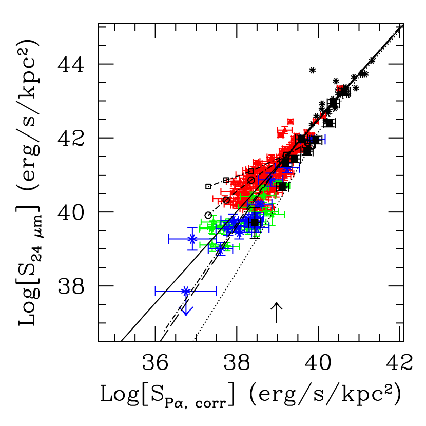
Figure 9: Luminosity surface density at 24 $\mu$m as a function of the extinction–corrected Pa$\alpha$ LSD for the same datapoints as Figure 4 (after removal of the Sy 2 nuclei, the foreground and background sources, and the NGC5033 HII knots data, leaving 164 independent datapoints in the high metallicity HII knot subsample). The continuous line shows the best linear fit through the high metallicity HII knots, from Figure 4. Models of infrared and ionized gas emission are superimposed on the data, for a variety of star formation histories, stellar population ages, and metallicity (see Appendix). Models with solar metallicity (Z=Z_⊙) ISM and stellar populations include: 100 Myr–old constant star formation (SFR/area=4$\times$10^-5–4 M_⊙ yr^-1 kpc^-2, long–dash line); instantaneous burst with variable mass (10³–10⁸ M_⊙ kpc^-2) and color–excess, and constant age of 4 Myr (dot–dashed line); instantaneous bursts with constant mass (10⁶ M_⊙ kpc^-2) and variable age, and both variable color excess (dot–dashed line with empty circles) and constant color excess (E(B$-$V)=2 mag, dot–dashed line with empty squares). The circle and square symbols mark the population ages, right–to–left: 0.01, 2, 4, 6, 8, 10 Myr. The dotted line marks a 1/10 Z_⊙ model of constant star formation over the past 100 Myr. The upward–pointing arrow marks the approximate luminosity where the transition between single–photon heating and thermal equilibrium heating for the dust begins to occur.

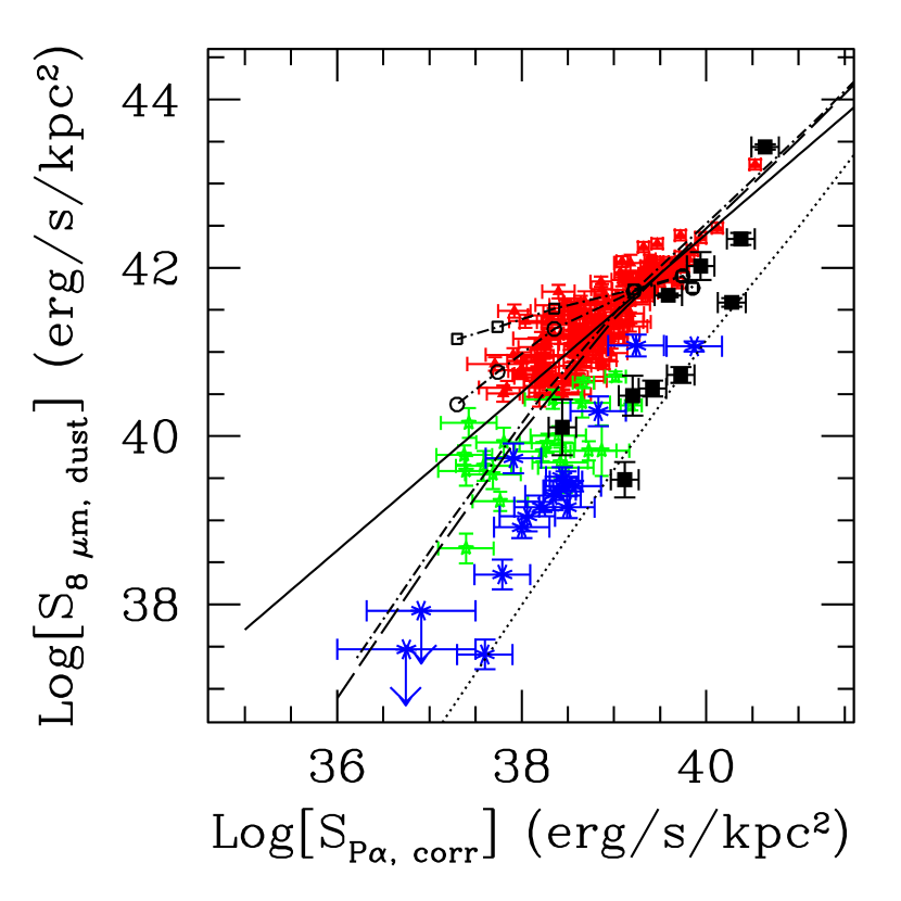
Figure 10: Luminosity surface density at 8 $\mu$m as a function of the extinction–corrected Pa$\alpha$ LSD for the same regions/galaxies as Figure 9 (minus the LIRGs). The continuous line is the best linear fit through the high metallicity HII knots, as in Figure 3. Models of infrared and ionized gas emission are the same as Figure 9.

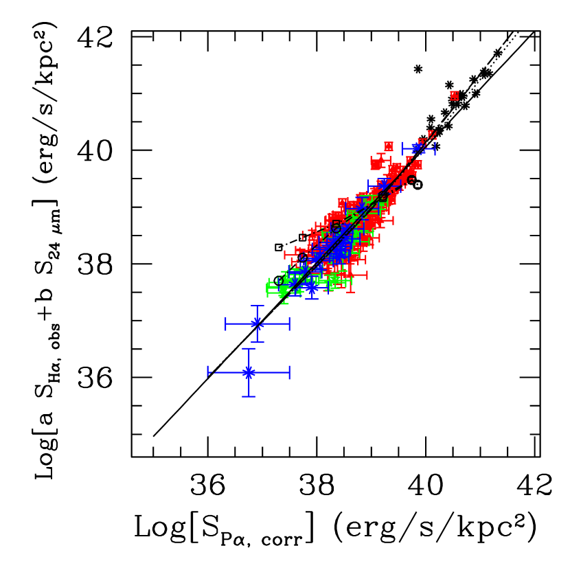
Figure 11: Combined–optical/mid–IR LSD as a function of the extinction–corrected Pa$\alpha$ LSD for the same data as Figure 9. The continuous line is the best linear fit through the high metallicity HII knots, as in Figure 7. Models of infrared and ionized gas emission are the same as Figure 9.

The basic approach adopts a range of plausible stellar populations for our HII knots (and starburst galaxies), in terms of star formation histories, stellar population ages, and metallicities (2005 update of Starburst99, Leitherer et al., 1999). Simple assumptions are also made for the ISM structure and metal content. The intrinsic stellar populations are then dust–attenuated according to empirical recipes (Calzetti, Kinney & Storchi–Bergmann, 1994; Meurer, Heckman & Calzetti, 1999; Calzetti et al., 2000; Calzetti, 2001) to provide a ‘predicted’ infrared emission, S_IR. As the stellar populations probed in our analysis range from groupings of a few to several HII regions for the HII knots to populations with extended star formation histories in the case of starbursts and LIRGs, both instantaneous bursts and constant star formation populations are included. The total infrared emission will, in general, depend not only on the adopted stellar population, but also on the extinction curve and the dust geometry. Since for the last two parameters, we make a simplifying assumption and use the prescription of Calzetti (2001); the impact of varying the dust geometry is discussed in section A.4. For the spectral energy distribution (SED) of the infrared emission, S_IR, we adopt the model of Draine & Li (2006), according to which the fraction of IR power emerging in the IRAC 8 $\mu$m and MIPS 24 $\mu$m bands is a function of the starlight intensity. We determine (section A.2) the range of starlight intensities corresponding to the model stellar populations we are considering, so to obtain a direct correlation between the Pa$\alpha$ LSD and the fraction of IR light emerging in the two mid–IR bands. Since our HII knots follow the well known correlation between SFR and extinction (Section A.1 and Wang & Heckman, 1996; Heckman et al., 1998; Hopkins et al., 2001; Calzetti, 2001; Moustakas, Kennicutt & Tremonti, 2006), which we parametrize as a relation between color excess E(B$-$V) (section 3.2) and the ionizing photon rate per unit area $\Sigma_{ion}$, we use this relation to link the stellar population models to the dust attenuation model, and eliminate one degree of freedom in our models. Model parameters that we allow to vary are the star formation history of the stellar populations (bursts or constant star formation), their age (0–10 Myr for instantanous bursts, the range chosen to ensure presence of significant ionizing photon rate, Leitherer et al. (1999); 6–100 Myr for constant star formation), the mass (10³–10⁸ M_⊙) or SFR (4$\times$10^-5–4 M_⊙ yr^-1) of the stellar cluster(s) associated with the HII knot or starburst galaxy, and the metallicity of both the population and the interstellar medium (0.1–1 Z_⊙). Figures 9–11 show the basic results from the comparison between the models described so far and our data for the 8 $\mu$m, 24 $\mu$m, and combined optical/mid–IR emission from HII knots and star–forming galaxies.

The larger–than–unity slope of the 24 $\mu$m versus Pa$\alpha$ LSD (in log–log scale, Figure 9) is a natural outcome of the models in the high luminosity surface density regime, Log(S_Paα,obs)$>$39, and is an effect of the ‘hotter’ IR SEDs for increasing starlight intensity. In other words, regions with higher Pa$\alpha$ LSD emit proportionally more of their infrared energy into the 24 $\mu$m band, because the peak of the IR SED moves towards shorter wavelengths (higher ‘effective’ dust temperatures, see Appendix and Draine & Li (2006)). The models also predict a slightly larger than unity value for the slope of the 8 $\mu$m LSD correlation, which is steeper than that of the HII knot data (Figure 10), but is roughly consistent with the slope of the integrated measures.

The models account well for the linear relation of the combined optical/mid–IR LSD with the Pa$\alpha$ LSD (Figure 11), for luminosity surface densities S${}_{Pa\alpha,corr}<$10⁴⁰ erg s^-1 kpc^-2. At high luminosity surface density, the models for the combined LSDs depart from a linear relationship, as increased starlight intensities are expected to raise the temperatures of the larger grains so that the fraction of the absorbed energy re–radiated at 24 $\mu$m (which is, at these high LSDs, the dominant contribution to equation 5) increases. The LIRGs data, that populate the high LSD regime in our plot, do indeed confirm observationally the deviation from the extrapolation of the best fit line; they show a steeper–than–one slope, in qualitative agreement with the models’ expectations (Figure 11).

At the high luminosity end (LIRGs and brighter), an additional effect that can contribute to the deviation from the slope of unity observed in Figure 11 and the steeper–than—unity slope of Figure 9 is the competition between the dust and the gas for the absorption of some of the ionizing photons. In the high luminosity regime, star formation occurs in environments of increasing density, e.g., ultracompact HII regions (Rigby & Rieke, 2004), and the dust absorbs the ionizing photons before they can excite the gas. In this regime, standard extinction–correction methods become progressively less effective at recovering the intrinsic Pa$\alpha$ emission, and will produce an underestimate of the hydrogen emission line LSD at constant 24 $\mu$m LSD (section A4). The impact of this effect on our data is unclear (and currently not included in our models), although it may be relatively small as the bulk of the observed trends is fully accounted for by our baseline model.

Instantaneous burst populations and constant star formation populations produce mostly degenerate models for all three mid–IR quantities (Figures 9–11). A young, 4 Myr old, instantaneous burst population in the mass range $\sim$10³–10⁸ M_⊙ provides similar model lines as a constant star formation model forming stars since 100 Myr and with SFR in the range 4$\times$10^-5–4 M_⊙ yr^-1.

However, even the high–metallicity HII knots in Figures 9–10 show a fairly large dispersion around the mean trends described above, with a clear increase of the dispersion around the mean S${}_{8~{}\mu m,\ dust}$ and S${}_{24~{}\mu m}$ values for S${}_{Pa\alpha,corr}\leq$10³⁹ erg s^-1 kpc^-2. Furthermore, in this Pa$\alpha$ LSD regime, most of the 8 $\mu$m and 24 $\mu$m emission from the high–metallicity HII knots is located above the baseline model lines, i.e., the models underpredict the mean values of the mid–IR emission (Figures 9–10). The ‘downward’ curvature of the models is a direct product of the increasing transparency of the interstellar medium for decreasing ionizing photon rate density and, from equation A2, decreasing dust amount. With a more transparent medium, proportionally less IR radiation is produced. The medium is still thick to Lyman continuum photons, and the ionized hydrogen emission lines are still a measure of the total number of ionizing photons in the region. An additional parameter is thus required to account for both the large scatter of the datapoints around the mean trends and the large number of high–metallicity datapoints above the model lines for the S${}_{8\mu m,\ dust}$ and S_24μm LSD plots. This second parameter appears to be the age of the stellar population. Ageing bursts between $\sim$0.01 Myr and $\sim$8 Myr produce a decreasing number of ionizing photons, while at the same time remaining luminous at UV–optical wavelengths (the major contributors to the IR emission). Figures 9–11 show that the ‘flaring’ of the high–metallicity HII knots datapoints around the mean value for decreasing Pa$\alpha$ LSD is compatible with the ‘flaring’ of the ageing burst models. Such ageing populations can also account for the data points above the mean trends in Figures 9 and 10.

The presence of ageing bursts is a sufficient (and physically expected), but not a necessary, condition to account for the dispersion in the data. As briefly discussed in the Appendix (section A.4), different assumptions from our default one about the average dust geometry can also produce a higher mid–IR emission than our fiducial model lines. For instance, presence of ultracompact HII regions within our HII knots will produce higher IR emission at fixed S_Paα,corr than expected from the models. This is a consequence of the higher opacity of such regions, for which the use of the H$\alpha$/Pa$\alpha$ ratio to recover the intrinsic line fluxes will lead to an underestimate of the intrinsic Pa$\alpha$ luminosity in the region. Recently, Dale et al. (2006) have shown that for local star–forming galaxies the UV/IR ratio is heavily determined by the morphology of the 24 $\mu$m dust emission, in particular by the ‘clumpiness’ of such emission, which therefore determines the escape fraction of UV photons from star–forming regions. A clumpy configuration of dust is, however, well described by the empirical recipes of dust extinction and attenuation used in the present work (Calzetti, Kinney & Storchi–Bergmann, 1994; Meurer, Heckman & Calzetti, 1999; Calzetti, 2001).

For the combined optical/mid–IR LSD, the models are degenerate as a function of metallicity (Figure 11). This is not surprising if the main driver of the discrepancy between the high and low metallicity S_24μm at fixed Pa$\alpha$ LSD is the larger medium transparency, i.e., lower dust column density, in the lower metallicity data (equations A2 and A4). This is indeed the case (Figure 9): the separation at low Pa$\alpha$ LSD between the solar metallicity and the 1/10th solar metallicity model lines is mostly due to the metallicity scaling factor in equations A2 and A4, and, to a much smaller extent, to the difference in metallicity of the two stellar populations. The 1/10th metallicity model line in Figure 9 provides the lower envelope to the data; most of the galaxies in our sample are above 1/10th solar in metallicity, and thus are expected to lie above this model line.

This result lends credence to the use of a combination of S_24μm and S_Hα,obs (equation 5 and Kennicutt et al., 2007a) as an effective tool for measuring the ionizing photon rates, and, ultimately, SFRs, at least up to Pa$\alpha$ LSDs $\approx$10⁴⁰–10⁴¹ erg s^-1 kpc^-2. In this framework, S_24μm probes the obscured star formation, and the only metallicity effects are those induced by reduced opacity; conversely, S_Hα,obs probes that part of the star formation unabsorbed by the dust, independent of the gas metallicity. The behavior of the models in Figure 11 shows little difference between different parameters choices, at least within our data uncertainties, and they reproduce the main trend of the data reasonably well.

The discrepancy observed between the high metallicity and low metallicity S${}_{8\mu m,\ dust}$ data at fixed Pa$\alpha$ LSD requires one additional ingredient, together with the increased transparency of the medium. Draine & Li (2006) have suggested that the fraction of low–mass PAH molecules present in the dust mixture decreases for decreasing metallicity. In the Appendix, we show that the two ingredients (increased medium transparency and decrease of low–mass PAH molecule fraction) provide comparable contributions to the depression of the 8 $\mu$m emission, and the two together produce the expected lower envelope to the datapoints in Figure 10.

8 Discussion

The scope of this study has been to investigate the extent of the regime of applicability of mid–IR emission as a SFR tracer, to use models to reproduce the main characteristics of the data, and to investigate reasons for any limitation we have encountered. The general trend of mid–infrared luminosity surface densities to correlate with the ionizing photon rates or with SFR tracers had already been found by a number of authors (for some of the most recent results, see Roussel et al., 2001; Förster Schreiber et al., 2004; Boselli, Lequeux & Gavazzi, 2004; Calzetti et al., 2005; Wu et al., 2005; Alonso–Herrero et al., 2006).

8.1 The Combined Optical/Mid–IR SFR Indicator

Of the three indicators investigated here, the linear combination of the observed H$\alpha$ and the 24 $\mu$m emission is the one most tightly correlated with the extinction–corrected Pa$\alpha$ emission. The linear relation between the combined optical/mid–IR emission and the SFR as traced by S_Paα,corr is common to all galaxies investigated, independent of their metallicity. The most straightforward interpretation (Kennicutt et al., 2007a) is that the 24 $\mu$m emission traces the dust–obscured star–formation, while the observed H$\alpha$ emission traces the unobscured one. The combination of the two, thus, recovers all the star formation in a region. This interpretation is confirmed by the models investigated in the previous section, which also suggest the trend to be relatively independent of the characteristics of the underlying star–forming population. The deviations from the linear relation (i.e., from a slope of 1 in log–log scale, Figure 11) observed at luminosities larger than S${}_{Pa\alpha,corr}>$10⁴⁰–10⁴¹ erg s^-1 kpc^-2 are also consistent with the models’ expectations: as the 24 $\mu$m emission starts dominating the luminosity budget, the same physical mechanism producing the S${}_{24~{}\mu m}$–versus–S_Paα,corr trend also produces that of the combined optical/mid–IR indicator. We speculate that this mechanism (see below) is the emission from grains with approximately steady temperatures, rather than transiently–heated grains, that come into play at high dust temperatures, and which causes the ratio of 24 $\mu$m/IR to deviate from a constant value at low starlight intensities to one that increases with the starlight intensity.

Using our baseline best–fitting model of 100 Myr constant SFR, for solar metallicity and the stellar initial mass function (IMF) described in section A.2, the conversion between SFR and H$\alpha$ luminosity is:

$$SFR(M_{\odot}~{}yr^{-1})=5.3\times 10^{-42}L(H\alpha)_{corr}(erg~{}s^{-1}).$$ (6)

Variations of $\pm$20% over the constant in this relation are present for younger ages and metallicities down to $\sim$1/5th solar. The $\sim$50% difference between the calibration in Equation 6 and that of Kennicutt (1998a) is mainly due to differences in the stellar IMF assumptions (59%), with a small contribution in the opposite direction coming from different assumptions on the stellar populations (100 Myr in our case versus infinite age in Kennicutt (1998a), which gives a 6% decrease to the discrepancy given by the different IMFs). Using equations 5 and 6:

$$SFR(M_{\odot}~{}yr^{-1})=5.3\times 10^{-42}[L(H\alpha)_{obs}+(0.031\pm 0.006)L(24~{}\mu m)],$$ (7)

where the luminosities are in erg s^-1, and L(24 $\mu$m) is expressed as $\nu$L($\nu$). This calibration does not change if the luminosities are measured over a substantial area of the galaxy (in our case the inner $\sim$0.8 to $\sim$5.1 kpc), rather than in smaller regions hugging the HII complexes that produce the ionizing radiation (Figures 7 and 8). However, the potential non–linearity at large LSDs is an important caveat.

8.2 The 24 $\mu$m SFR Indicator

Conversely, neither the 8 $\mu$m emission nor the 24 $\mu$m emission alone are linearly correlated with the number of ionizing photons that are measured in a region. The non–linearity at high 24 $\mu$m luminosity is a direct consequence of the increasing dust temperature for more actively star forming objects (Li & Draine, 2001; Draine & Li, 2006; Dale et al., 2001); higher dust temperatures correspond to higher fractions of the infrared emission emerging at mid–IR wavelengths. Following Draine & Li (2006), in the regime of low stellar intensities (low SFRs in our actively star–forming regions, or roughly S${}_{Pa\alpha,corr}<10^{39}$ erg s^-1 kpc^-2), most of the 24 $\mu$m emission comes from single photon transient heating of small grains. In this case, the 24 $\mu$m photon flux is directly proportional to the stellar UV photon flux (or any other photon capable of single photon heating). Thus, the 24 $\mu$m emission counts stellar UV/optical photons, while the Pa$\alpha$ counts the Lyman continuum photons; since there is proportionality between the two types of photons, the expectation is for a linear scaling between 24 $\mu$m emission and Pa$\alpha$ emission. However, this regime corresponds to the Pa$\alpha$ LSD range where the decrease of dust opacity also decreases non–linearly with the amount of stellar energy re-processed by dust in the infrared. At high Pa$\alpha$ LSDs, hence high stellar intensities, the dust absorbing most of the stellar photons is warm. There is thus an increasing contribution to the 24 $\mu$m emission from larger, warm grains (the Wien side of the emission from grains), which leads to a non–linear dependence of the 24 $\mu$m flux on the stellar flux. This is in agreement with the conclusions of Smith et al. (2007), which observe a decrease of the PAH/24 $\mu$m luminosity ratio for increasing 24 $\mu$m/70 $\mu$m luminosity ratio; this dependence is highly suggestive of an increasing contribution of warm dust to the 24 $\mu$m emission.

The observed non–linearity in the 24 $\mu$m versus Pa$\alpha$ relation, S${}_{24~{}\mu m}\propto$S${}_{Pa\alpha,corr}^{1.23}$, also argues against the case that the high LSDs values measured of our apertures may be due to the cumulative contribution of many faint HII regions, rather than a few, increasingly bright HII regions. In the case of many faint HII regions (low stellar intensities, and, therefore, single photon heating) we should expect the 24 $\mu$m LSD to scale linearly with the Pa$\alpha$ LSD at the high end. The observed non–linear behavior argues in favor of the high luminosity end to be contributed mainly by intrinsically bright regions, although presence of apertures with many faint HII regions cumulatively giving a high LSD may still be present and contribute to the scatter of the datapoints around the mean trend.

At low metallicities, the deviation from a linear correlation is due to lower opacities for decreasing metal content, and thus column densities (Walter et al., 2007). The effect has been well known since the early IRAS observations (Helou et al., 1988): as the metallicity decreases, regions become proportionally more transparent and emit less in the infrared as a larger fraction of the radiation escapes the area unabsorbed by dust. This accounts for the underluminosity of the medium in low metallicity regions in correspondingly intense ionizing fields. Using the 24 $\mu$m luminosity as a SFR tracer is thus subject to many caveats, including that lower metallicity sources will generally be more transparent than their metal-rich counterparts, and the infrared emission will typically underestimate their SFR by a factor $\sim$2–4.

The non–linear correlation between S${}_{24~{}\mu m}$ and S_Paα,corr requires some care for deriving SFR calibrations. From equation 3, and using equation 6, we derive a SFR density (SFR per unit area) calibration:

$$\Sigma_{SFR}(M_{\odot}~{}yr^{-1}~{}kpc^{-2})=1.56\times 10^{-35}[S_{24~{}\mu m}\ (erg~{}s^{-1}~{}kpc^{-2})]^{0.8104}.$$ (8)

In order to derive a calibration for SFRs, we convert our LSDs into luminosities, and the resulting best fit through the high–metallicity datapoints produces:

$$SFR(M_{\odot}~{}yr^{-1})=1.27\times 10^{-38}[L_{24~{}\mu m}\ (erg~{}s^{-1})]^{0.8850}.$$ (9)

The exponents of equations 8 and 9 are the same within the 3 $\sigma$ error (the combined 1 $\sigma$ uncertainty is 0.03). Equation 9 is closer to a linear relation than equation 8, because we add a distance effect when using luminosities (which depend on the distance squared). A large sample of regions with comparable distances may be needed to fully sort out intrinsic effects from distance–related effects. Both relations are derived from best bi-linear fitting of data on HII knots, but their extrapolations account for the observed properties of LIRGs as well. Additionally, when considering more extended galactic regions or starburst galaxies, equation 8 does not change significantly (Figures 4 and 8). Equations 8 and 9 may thus be applicable to galaxies in general whose energy output is dominated by recent star formation.

Equation 9 is very similar to that of Alonso–Herrero et al. (2006), who have derived a SFR calibration for the 24 $\mu$m luminosity using a sample of Ultraluminous Infrared Galaxies, LIRGs, and NGC5194. The difference in the calibration constant between our equation 9 and the calibration of Alonso–Herrero et al. (2006) is entirely due to the slight difference in exponent between the two relations, and the different SFR–L(H$\alpha$) calibrations used here and in that work. Perez–Gonzalez et al. (2006) find a lower exponent, $\sim$0.77, than the one in equation 9, about a 4 $\sigma$ difference; however, their result is based on line emitting regions in just two galaxies, NGC5194 and NGC3031.

8.3 The 8 $\mu$m Emission

The analysis of the HII knots in M51 has shown a general, non–linear correlation between the 8 $\mu$m and the Pa$\alpha$ emission (with exponent 0.79, Calzetti et al., 2005). The present study similarly recovers a non–linear behavior for the high–metallicity data, albeit less extreme than in the M51 case: S${}_{8\mu m,\ dust}\propto$ S${}_{Pa\alpha,corr}^{0.94}$. Our simple Z=Z_⊙ models also predict a non–linear correlation between the 8 $\mu$m and Pa$\alpha$ emission, but with an exponent slightly above unity. Therefore, the gap between observations and expectations is even wider than a simple deviation from a linear correlation; with our uncertainties, the discrepancy is at the 10 $\sigma$ level. This level of discrepancy remains unchanged when other uncertainties, e.g., on the dust modelling and on the correlation between dust attenuation and number of ionizing photons (see Appendix), are included. In contrast, the same simple models are quite successful at explaining the observed trend of S${}_{24~{}\mu m}$. We conclude that the 8 $\mu$m emission as measured within our apertures must include additional contributions that are not included in our simplified models.

Mechanisms that can produce a lower–than–expected slope in a correlation between S${}_{8\mu m,\ dust}$ and S_Paα,corr include the potential contamination of our measurements by the diffuse emission from the general galactic radiation field (Li & Draine, 2002; Haas, Klaas & Bianchi, 2002; Boselli, Lequeux & Gavazzi, 2004; Peeters, Spoon & Tielens, 2004; Wu et al., 2005; Mattioda et al., 2005) and/or destruction/fragmentation of the 8 $\mu$m emission carriers (Boulanger et al., 1988, 1990; Helou, Ryter & Soifer, 1991; Houck et al., 2004; Pety et al., 2005). In the case of destruction or fragmentation of the PAH emitters at 8 $\mu$m, the brightest HII regions will show a deficiency in the 8 $\mu$m luminosity relative to the fainter regions. In the case where non–ionizing populations, as well as ionizing ones, heat the 8 $\mu$m dust carriers, the contribution of the former to the S${}_{8\mu m,\ dust}$ measurements within our apertures will become proportionally larger as the HII regions become fainter (decreasing S_Paα,corr), again flattening the observed trend. Finally, if the volume filling factor of the 8 $\mu$m luminosity originating in the PDRs evolves differently from that of the HII regions (or other inhomogeneities in the 8 $\mu$m emission distribution are present) as the HII region’s luminosity increases (Förster Schreiber et al., 2004; Helou et al., 2004), the net result will also be a lower–than–expected exponent between S${}_{8\mu m,\ dust}$ and S_Paα,corr.

The correlation exponent predicted by models of the 8 $\mu$m LSD versus Pa$\alpha$ LSD is better matched by the data of large–scale (multiple–kpc) measurements of the centers of the high–metallicity galaxies (Figure 8). There is, however, an offset between models and observations, in the sense that the data imply about 65%–100% more 8 $\mu$m emission than expectations from models. This result argues in favor of one of the mechanisms described above: the presence within our apertures of diffuse 8 $\mu$m emission unrelated to the current star formation. Indeed the result can be explained if stellar populations other than those related to the current star formation can heat the carriers of the 8 $\mu$m emission, and their contribution becomes proportionally larger than that of the ionizing populations as the size of the sampled region within each galaxy increases.

The underluminosity of the 8 $\mu$m emission at low metallicities (Boselli, Lequeux & Gavazzi, 2004; Engelbracht et al., 2005; Hogg et al., 2005; Galliano et al., 2005; Rosenberg et al., 2006; Madden et al., 2006; Wu et al., 2006; Draine et al., 2007) is not a function of the intensity of the radiation field (Figure 6). Metal–poor regions as bright (in ionizing photon density) as metal–rich region have, neverthless, 8 $\mu$m LSDs that are almost an order of magnitude lower. The most metal–poor regions can be as much as a factor of 30 fainter at 8 $\mu$m than their metal–rich counterparts at fixed Pa$\alpha$ LSD. In addition to the decrease of the dust opacity with metallicity (the same effect present for the 24 $\mu$m), the data require a second ingredient to account for the underluminosity at 8 $\mu$m. The second ingredient, from the models of Draine & Li (2006), is the decrease of the mass fraction of the low–mass polycyclic aromatic hydrocarbon molecules in the dust mixture for decreasing metallicity. This decrease affects selectively more the 8 $\mu$m emission than the 24 $\mu$m emission, as the former has a larger fraction of its flux contributed by single–photon–excitation of PAHs. The models, indeed, account reasonably well for the observed deficiency of the 8 $\mu$m flux in metal–poor objects (Draine et al., 2007). A possible mechanism to reduce the mass fraction of PAH molecules in the low–metallicity galaxies is destruction by the hard radiation field in those galaxies (e.g., Madden et al., 2006; Wu et al., 2006), although these molecules have proven surprisingly robust (Engelbracht et al., 2006). An alternative possibility to destruction is that the lowest metallicity galaxies may not have formed the carriers of the aromatic features in the first place (Engelbracht et al., 2005; Dwek, 2004).

The correlation that exists between Log[S${}_{8~{}\mu m,\ dust}$] and Log[S_Paα,corr] for the metal–rich regions (equation 3) is statistically as significant as those existing for the 24 $\mu$m and for the combined optical/mid–IR luminosity. However, there are many caveats in using such correlation to trace SFRs with the 8 $\mu$m emission. First and foremost, stellar populations other than those which are currently forming stars contribute to the mid–infrared emission: thus, a calibration of the 8 $\mu$m emission as a SFR tracer will depend on the galactic area probed, and, possibly, on the ratio between current and past (or recent–past) star formation. A second limitation is the extreme sensitivity of the 8 $\mu$m emission to metallicity, which is about an order of magnitude larger than what observed for the 24 $\mu$m emission.

In all cases, the presence of Active Galactic Nuclei in unresolved galaxies will complicate the use of the mid–IR band emission for SFR determinations. Galaxies in the SINGS sample that contain central non–thermal sources (Sy2s or LINERs) show prominent nuclear emission in the mid–IR bands; in our case, the 8 $\mu$m and 24 $\mu$m emission from the non–thermal nuclei tends to be as bright as some of the brightest HII knots in their host galaxies (Figures 3 and 4).

9 Summary and Conclusions

The analysis of the mid–infrared emission, at the Spitzer’s IRAC 8 $\mu$m and MIPS 24 $\mu$m wavelengths, from a set of local galaxies drawn from the SINGS sample has shown that their viability as SFR indicators is subject to a number of caveats. The calibrations given in this work, provided the caveats are taken into account, should however be useful for measurements of SFRs in actively star–forming galaxies using their observed mid–infrared emission, in the absence of prominent central AGNs.

The most robust of the indicators analyzed in this study is the one proposed by Kennicutt et al. (2007a), which combines the observed H$\alpha$ and 24 $\mu$m luminosities as probes of the total number of ionizing photons present in a region. Here we present a calibration (equation 7) for that relation that is based on measurements of 220 HII regions/complexes in 33 nearby galaxies. Comparisons with models suggest that the calibration should be applicable to large systems or galaxies whose energy output is dominated by young stellar populations, up to at least luminosity surface densities of S${}_{Pa\alpha,corr}>$10⁴⁰–10⁴¹ erg s^-1 kpc^-2.

Second–best is the 24 $\mu$m emission alone, which, although robust (within the limits of our analysis) for metal–rich objects, shows substantial deviations, at the level of factors 2–4, from the mean trend for decreasing metallicity. Models can account for the observed deviations as an effect of the increased transparency of the medium for lower metal abundances (less dust means less infrared emission). The calibration presented here (equations 8 and 9) is non–linear and reflects both observations and expectations from models. The calibration is appropriate for metal–rich HII regions or starbursts, and caution should be exercised when applying it to extended star–forming galaxies (Kennicutt & Moustakas, 2006) or to metal–poor targets. In particular, galaxies with a prominent contribution from non–star–forming populations to the integrated light may receive a yet unquantified contribution to the 24 $\mu$m emission from a diffuse component. This diffuse component would not be directly related to star formation and may be in the single–photon–heating regime; its presence would add to the integrated 24 $\mu$m emission and would alter the calibration of this emission for SFR measurements.

We do not present a calibration of the SFR based on the 8 $\mu$m emission, as emission at this wavelength shows strong dependence not only on metallicity (more than an order of magnitude), but also on the size (about a factor of 2) and, possibly, star formation history of the region being measured. It should be remarked, however, that when measurements are limited to regions of star formation with a narrow spread in metallicity around the solar value, the 8 $\mu$m emission shows a correlation that is almost linear with the ionizing photon rate.

The mean trends between the mid–IR emission (at 8 $\mu$m, 24 $\mu$m, and combined optical/mid–IR) and the ionizing photon tracer Pa$\alpha$ are well accounted for by either a 4 Myr old burst of star formation or a $>$100 Myr old constant star formation model; this provides a measure of the degeneracies in the population models, but also a measure of the general applicability of the calibrations discussed here to both star–forming regions within galaxies and whole star–formation–dominated galaxies.

In all cases, the spread around the mean trends has a r.m.s. of $\sim$0.3 dex (each side). This spread is well accounted for by allowing stellar populations with a range of ages, between 0 Myr and 8 Myr, to produce the observed emission. The older stellar populations can account for HII knots with high mid–IR emission relative to the ionizing photons density, although more complex dust geometries than those analyzed here can also contribute to the spread.

Our analysis has concentrated on HII knots and starburst galaxies, where star–forming stellar populations dominate over more evolved populations in the bolometric output of the galaxy. However, the contribution of non–ionizing stellar populations to the heating of the dust emitting in the mid–IR region needs to be fully quantified, in order to test the applicability of (or derive modifications for) the SFR calibrations presented in this work to more general environments, such as quiescently star forming galaxies. This is the subject of a future investigation which employs the SINGS and other star–forming galaxies as testbeds (Kennicutt & Moustakas, 2006).

Appendix A Models of Dust Absorption and Emission

A.1 The Energy Balance

To aid the interpretation of the observed correlations between the mid-infrared emission and the Pa$\alpha$ emission (a tracer of the number of ionizing photons), we build a simple model of dust attenuation of the spectral energy distribution of a young stellar populations at UV–to–nearIR wavelengths, with the prescription that the dust absorbed energy is re–emitted in the mid/farIR with a spectral energy distribution that follows the Draine & Li (2006) models. Ideally, the ‘perfect’ estimator of SFR should correlate linearly with the SFR itself. We have seen in section 6 that this is not the case for S${}_{24~{}\mu m}$ and S${}_{8~{}\mu m,\ dust}$; a legitimate question is whether the nature of the observed non–linearity is such to jeopardize a reliable use of the mid–IR emission as a SFR indicator. Thus, our main interest in this section is to understand whether a heuristic model can account for the observed trends as a function of both luminosity surface density and metallicity, and is able to:

• reproduce the observed mid–IR emission level and its trend as a function of the Pa$\alpha$ LSD with simple prescriptions for the stellar emission spectrum, dust geometry, and ISM metallicity in the regions;

• provide a physical explanation for the non–linear correlations between the mid–IR LSDs and the line emission LSD;

• match overall expectations on the age of the stellar populations in the ‘HII knots’.

For the simplest assumption that the dust extinction is described as an effective foreground attenuation A($\lambda$) (Calzetti, Kinney & Storchi–Bergmann, 1994; Meurer, Heckman & Calzetti, 1999), the bolometric (3–1000 $\mu$m) infrared luminosity L_IR is given by:

$$L_{IR}=\int_{0}^{\infty}F_{S}(\lambda)[1-10^{-0.4A(\lambda)}]d\lambda,$$ (A1)

where F_S($\lambda$) is the stellar light SED. We use the ‘foreground attenuation’ as a working hypothesis, since it enables us to account for both absorption and scattering (in and out of the line of sight) of the stellar light by dust with a simple expression (Calzetti, Kinney & Storchi–Bergmann, 1994; Calzetti et al., 2000). Potential limitations to this assumption will be discussed in section A.4.

Our general results indicate a correlation between the mid–infrared emission and the number of ionizing photons in HII knots. Similar correlations have been observed for whole galaxies (e.g., Roussel et al., 2001; Förster Schreiber et al., 2004; Wu et al., 2005; Alonso–Herrero et al., 2006), and are qualitatively not dissimilar from the correlation between the bolometric infrared emission and the SFR derived for galaxies dominated by young stellar populations using IRAS data (Lonsdale Persson & Helou, 1987; Rowan–Robinson & Crawford, 1989; Devereux & Young, 1990; Sauvage & Thuan, 1992). Equation A1 shows that such correlations are mediated by the dust attenuation A($\lambda$); indeed, starburst and star–forming galaxies have been shown to be redder and to suffer generally higher dust attenuation as their SFRs increase (Wang & Heckman, 1996; Heckman et al., 1998; Hopkins et al., 2001; Calzetti, 2001; Moustakas, Kennicutt & Tremonti, 2006). This general trend is also shown by the HII knots in our sample. A plot of the color excess E(B$-$V) , derived from the H$\alpha$/Pa$\alpha$ ratios of individual HII knots, as a function of the Pa$\alpha$ LSD is shown in Figure 12, together with the best fit through the datapoints. The data in Figure 12 are for the high metallicity subsample, the group with the largest number of datapoints and the widest range in color excess in our sample. If we introduce the ionizing photon rate per unit area, $\Sigma_{ion}$, in units of s^-1 kpc^-2 as derived directly from S_Paα,corr for case B recombination, then in solar metallicity regions E(B$-$V) is related to the ionizing photon rate via the best fit (bi–linear on the log of the quantities):

$$E(B-V)=0.21\ \biggr{(}{\Sigma_{ion}\over 10^{51}s^{-1}kpc^{-2}}\biggl{)}^{(0.61\pm 0.03)},$$ (A2)

where E(B$-$V) is in magnitudes. The correlation has 5.7 $\sigma$ significance, and is independent of the specifics of the stellar population (age, burst or constant star formation, etc.).

Some physical insights on the meaning of equation A2 can be gained by looking at the implications of the scaling laws of star formation. The Schmidt Law (Kennicutt, Edgar & Hodge, 1989; Kennicutt, 1998a) provides a way to relate the SFR density to the gas density in galaxies. Furthermore, in our own Galaxy, there is a tight correlation between the color excess E(B$-$V) and the gas (HI$+$H₂) column density (Bohlin, Savage & Drake, 1978). By combining the Schmidt Law, as derived locally for regions in NGC5194 (Kennicutt et al., 2007a), and the extinction–gas column density correlation, we get a relation between the color excess and the SFR density:

$$E(B-V)=10.30\ \gamma\ \Sigma_{SFR}^{0.64},$$ (A3)

where $\Sigma_{SFR}$ is in units of M_⊙ yr^-1 kpc^-2 and the factor $\gamma$ accounts for the fact that not all the gas (and the dust) is in front of the stars. Equation A3 can be readily related to equation A2, since the two exponents, 0.61 in the first and 0.64 in the second equation are formally the same number within the 1 $\sigma$ uncertainty of our fitting procedure (see, also, Figure 12). By fitting the data of Figure 12 with a straight line of fixed slope 0.64 (equation A3), we get an estimate of $\gamma=$0.4–0.45 for the constant star formation models, depending on the time elapsed since the onset of star formation (6–100 Myr). This value of $\gamma$ is very close to the mean value of 0.5 expected in the case the star formation is located on average at the mid–point of the gas column density.

Metallicity variations in the stellar populations produce small variations in equation A2. However, observations of the extinction to gas column density correlation for the Large and Small Magellanic Clouds suggest roughly linear scaling with metallicity (Koornneef & Code, 1981; Bouchet et al., 1985). This is likely to be the dominant dependence of equation A2 on metallicity, and we model it as a linear dependence on $Z$, the interstellar medium’s metallicity in solar units:

$$E(B-V)=0.21\ Z\ \biggr{(}{\Sigma_{ion}\over 10^{51}s^{-1}kpc^{-2}}\biggl{)}^{0.61},$$ (A4)

Although non–parametric (Spearman and Kendall) rank tests indicate that the data in Figure 12 deviate from the null (uncorrelated) hypothesis by 5.7 $\sigma$, the spread around the mean trend is still significant. The 90% boundary is located at (-0.4 dex, $+$0.5 dex) along the vertical axis. We will see in section A.4 that the large spread in Figure 12 has a small impact on the main conclusions of this Appendix. That said, it should be important to keep in mind that although the trends have a physical base in the combination of the Schmidt Law with the extinction–gas column density correlation (Heckman, T.M. 2004, private communication; Tremonti, C.A., 2006, private communication), individual variations remain important.

Equations A2 and A4 will be used in combination with equation A1 in the following sections to provide a heuristic description of the relation between ionizing photon rates (star formation rates) and monochromatic dust emission in our regions, in order to understand the broad trends observed in the data. Thus, equations A2 and A4 are derived from data and will be used to explain data, and the potential of circular argument should be addressed. The data in Figure 12 are completely independent of the data presented in Figures 3, 4, and 7. The color excess E(B$-$V) is derived from ionized gas emission, while the monochromatic dust emission is mainly due to stellar continuum emission. Equation A1 also requires independent assumptions on the underlying stellar population, and the dust geometry relative to both the stellar population and the ionized gas (see next section, Calzetti, Kinney & Storchi–Bergmann, 1994). Therefore, the use of the extinction–ionizing photons correlation of equations A2 and A4 is unlikely to automatically enforce a fit to the data in Figures 3, 4, and 7. Finally, we will see in section A.4 that equations A2 and A4 are not necessary to account for the observed data for Pa$\alpha$ LSDs above $\sim$3$\times$10³⁸ erg s^-1 kpc^-2.

A.2 Model Parameters

For F_S($\lambda$) in equation A1, we adopt the stellar population models of Starburst99 (2005 update; Leitherer et al., 1999). Since we are exploring the infrared emission of both HII knots and star–formation–dominated galaxies, we consider both bursts of star formation and constant star formation. Burst models are explored in the age range 0–10 Myr, as older ages do not produce enough ionizing photons to provide Pa$\alpha$–detectable HII knots in our data. As bursts age, the number of ionizing photons produced by the massive, short–lived stars, decreases, while the UV–optical stellar luminosity (the main contributor to the infrared emission) remains comparatively high, since it is contributed by lower–mass, longer–living stars. Thus, aging stellar populations produce high luminosity ratios L(IR)/L(Pa$\alpha$). For constant star formation, the representative case of a 100 Myr–duration model is considered. The difference between this model and a much younger case is the increase of optical and infrared light in the older model, due to the accumulation of previous–generations, low–mass, long–lived stars. The light from these older stars contributes to L(IR), but not to the ionizing photons budget. The net effect is that the 100 Myr constant star formation model produces about twice as much infrared emission as a, e.g., 6 Myr old case, for the same dust opacity. The variation between the 100 Myr and 1 Gyr models is about 6%. For the stellar IMF, we adopt the Starburst99 default, which consists of two power laws, with slope $-$1.3 in the range 0.1–0.5 M_⊙ and slope $-$2.3 in the range 0.5–120 M_⊙. The SFRs derived from this IMF are a factor 1.59 smaller than those derived from a Salpeter IMF in the range 0.1–100 M_⊙, for the same number of ionizing photons.

For the wavelength dependence of the dust attenuation in equation A1, A($\lambda$)=k($\lambda$) E(B$-$V), we adopt the starburst obscuration curve of Calzetti (2001) (see, also, Calzetti, Kinney & Storchi–Bergmann, 1994; Meurer, Heckman & Calzetti, 1999; Calzetti et al., 2000), which prescribes an attenuation of the stellar continuum a factor 0.44 that of the emission lines.

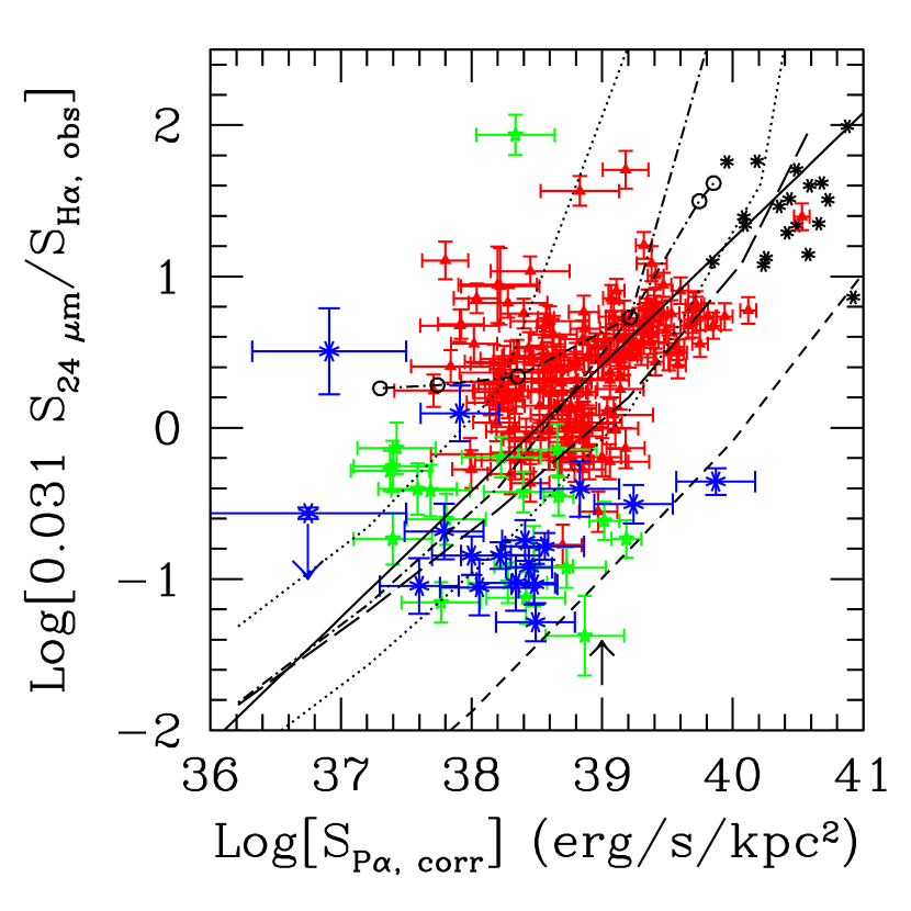
Figure 15: The ratio of the 24 $\mu$m to the observed H$\alpha$ LSD as a function of Pa$\alpha$, for the HII knots and LIRGs (Figure 9), compared with models. The datapoints are correlated with a $\sim$7 $\sigma$ significance; the continuous line is the best bi-linear fit through the data, and has slope $0.83$. Solar metallicity models include (Figure 9): instantaneous burst with variable mass (10³–10⁸ M_⊙) and color–excess, and constant age of 4 Myr (dot–dashed line); instantaneous burst with constant mass (10⁶ M_⊙), variable age and variable color excess (dot–dashed line with empty circles marking, right–to–left: 0.01, 2, 4, 6, 8, 10 Myr). The dotted lines mark the upper and lower boundaries to the 90-percentile region from Figure 12. The long-dash line is the model of homogeneous dust–stars mixture, with no differential extinction between gas and stars, from Figure 14. The short-dash line is the 1/10th solar metallicity model, and marks to lower envelope to the datapoints. The upward–pointing arrow marks the approximate luminosity where the transition between single–photon heating and thermal equilibrium heating for the dust begins to occur (Figure 9).

The fraction of the infrared luminosity that emerges in the IRAC 8 $\mu$m and MIPS 24 $\mu$m bands, L(8)/L(IR) and L(24)/L(IR), is from the model of Draine & Li (2006), which updates the model of Li & Draine (2001). At solar metallicity, the two papers provide consistent prescriptions for our case. The fraction of infrared light emitted in either 8 $\mu$m or 24 $\mu$m band increases non–linearly as a function of the starlight intensity (Figure 15 of Draine & Li (2006)); the ratios are flat at the low intensity end (single photon heating of dust) and rise sharply at higher intensities, producing ‘hotter’ infrared SEDs, i.e., peaked at shorter wavelengths. At solar metallicity, the dependence of L(8)/L(IR) as a function of the starlight intensity is much shallower than that of L(24)/L(IR); the former varies by 50% over the full range of intensities analyzed here, while the latter changes by more than a factor of 10. The results of Draine & Li (2006) are expressed as a function of the parameter U, the starlight intensity in units of the solar neighborhood value.

We relate the typical stellar radiation field in our HII knots to U using the individual HII regions detected in the HST Pa$\alpha$ image of the nearby (and, thus, better resolved), actively star–forming galaxy NGC6946. From the image we measure the sizes, defined as the radius of the circular area containing 80% of the Pa$\alpha$ emission in each region, and line emission values of the HII regions. Total luminous energies are derived by associating the range of stellar models described above to the measured line intensities, and energy densities are derived by dividing for the measured volumes. By extrapolating the observed quantities, we find that burst models with mass 10⁶ M_⊙ and ages $<$6 Myr or constant star formation models with SFR=1 M_⊙ yr^-1 (L${}_{Pa\alpha,corr}\lesssim$10⁴⁰ erg s^-1), with radii R$\approx$100 pc, produce average starlight intensities U$\sim$400–1200. The factor $\sim$3 variation in U accounts for two uncertainties in our derivation: (1) star forming regions have hotter SEDs than the local interstellar medium (Mathis, Mezger & Panagia, 1983), and (2) our stellar models and regions’ sizes cover a range of values/characteristics. The presence of dust absorption within the HII region and the conversion of some of the energy to free–free emission also contribute to the uncertainty (and some decrease) in U. However, the results described in the next section are fairly insensitive to the actual value of U, within the range of 3–4 uncertainty detailed above. The relation between number of ionizing photons and starlight intensity derived above suggests that, for constant radii of the HII regions, the transition from single–photon heating to thermal equilibrium heating for the 24 $\mu$m emission begins to occur at emission line intensities S${}_{Pa\alpha,corr}\approx$10³⁹ erg s^-1 kpc^-2.

The impact of metallicity variations is explored by considering how the infrared emission changes under the two conditions that the regions/galaxies have solar metallicity (Z=Z_⊙) and one-tenth solar metallicity (Z=1/10 Z_⊙). The latter value is at the low end of the metallicity range in our sample; our goal is, indeed, to model the lower envelope to the data. The metallicity enters in two components of equation A1. The first component is the stellar population model, for which we use two metallicity values: solar and 1/5 solar (Starburst99 does not provide models for our default 1/10 Z_⊙, and 1/5 Z_⊙ is the closest metallicity value for the stellar populations). The second component is the dependence of the color excess on metallicity, which we describe in a linear fashion via equation A4. Additional metallicity–dependent ingredients are the conversion from ionizing photon rate to hydrogen nebular line luminosity (at the $\sim$15% level; see section 3.2), and the fraction of infrared light emerging in the 8 $\mu$m and 24 $\mu$m bands. We use, again, the model of Draine & Li (2006) for the latter, with the assumption that variable metallicities have a major impact on the mass fraction of the polycyclic aromatic hydrocarbons in the dust mixture; this, in turn, affects the dust emission in the mid–infrared bands, mainly the IRAC 8 $\mu$m band, which results predominantly from single–photon–heating at low values of the starlight intensity. For reference, in the low–U regime, L(24)/L(IR) changes by about 60% and L(8)/L(IR) changes by an order of magnitude for a factor 10 variation in the abundance of small PAH; the differences become negligible at the high–U end (Draine & Li, 2006).

A.3 General Model Trends

In the extreme case that we have no dust in our region, equation A1 will be null, and there will be no relation between SFR (or ionizing photon rate) and dust emission. In the presence of even small amounts of dust, however, the relation established by equation A1 will produce a general trend, with details that depend on a host of parameter assumptions. At the lowest levels of dust extinction, the relation between L(IR) and the number of ionizing photons is non-linear, with an asymptotic exponent of 1.64 for our equations A1–A4; a linear relation is established only once the integral on the right–hand–side of equation A1 corresponds to most of the stellar energy. In other words, once the region contains enough dust that most of the stellar energy is absorbed and re–emitted in the IR, larger numbers of ionizing photons will linearly correspond to larger IR luminosities.

The impact of the stellar population parameters on the characteristics of the 8 $\mu$m and 24 $\mu$m emission has already been shown in Figures 9–11. Stellar populations undergoing constant star formation since 100 Myr in the range SFR=4$\times$10^-5–4 M_⊙ yr^-1 have equivalent characteristics to bursts of star formation of constant age 4 Myr and mass in the range M=10³–10⁸ M_⊙. For the burst models, the impact of age variation is investigated at constant cluster mass (10⁶ M_⊙) and in the two cases of constant or age-variable (equation A2) color excess. The general effect of increasing the age is to move the model curves towards smaller values of the ionizing photon rates for roughly constant IR emission, almost independently of assumptions on the variation (or constancy) of the color excess.

The introduction of the age–variable extinction (via equation A2), however, attempts to mimic the observation that aging HII regions tend to be less dust extincted than the younger HII regions, whether because the more evolved populations have shed the native cocoon or have migrated away from it through secular motions (Mayya & Prabhu, 1996). This also introduces a modest dependence of the IR SED and the fraction of infrared light emerging in the 8 $\mu$m and 24 $\mu$m bands on age, via changes in the starlight intensity that aging HII regions produce. However, the model does not include additional effects, such as the expansion of HII regions as they evolve, that will affect the IR SED via the decrease of the dust temperature.

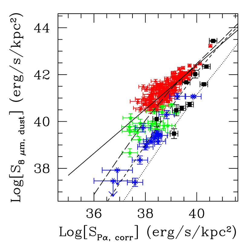
Figure 13: Models of dust absorption and emission for constant star formation populations and variable metallicity are compared with data, for the 8 $\mu$m (left) and the 24 $\mu$m (right) LSD as a function of the Pa$\alpha$ LSD. Symbols for the HII knots, the local starbursts, and the LIRGs are as in Figures 9–10. Straight continuous lines are the best fits through the high–metallicity HII knots, similar to the lines in Figures 3 and 4. All models are for a 100 Myr old constant star formation population, and include: solar metallicity (Z=Z_⊙, long–dash line); 1/10 Z_⊙ and standard low–mass PAH molecules fraction (short–dash line); 1/10 Z_⊙ and depleted low–mass PAH molecules fraction (dotted line Draine & Li, 2006). For the 24 $\mu$m–versus–Pa$\alpha$ plot, the effect of variations in the IR SED are also explored; in particular, our default assumption for the shape of the IR SED as a function of the starlight intensity (Draine & Li, 2006) is compared with the extreme assumption that the IR SED is constant, i.e., L(24)/L(IR)=const=0.3 (dot-dash line).

Not surprisingly, metallicity variations have a strong effect on the observed mid–IR emission as a function of the number of ionizing photons (Figure 13). For the 24 $\mu$m emission, most of the effect comes from the fact that the ISM is more transparent at lower metallicities. For the 8 $\mu$m emission, roughly equal contributions are given by the more transparent medium and by the decreased mass fraction of low–mass PAH molecules in the dust mixture (Figure 13, left).

The fiducial model for the IR SED as a function of starlight intensity (from Draine & Li, 2006) is compared with the more extreme assumption that the IR SED is constant for all analyzed regions/galaxies. For the assumption L(24)/L(IR)=const=0.3 (Figure 13, right), the model line has a different curvature from our fiducial one, starting with higher Log(S_24μm) values at low Pa$\alpha$ LSD, overshooting the datapoints in the LSD range Log(S_Paα,corr)=39–40, and converging to a slope of unity at higher LSD values. Our fiducial model appears to better reproduce the slope of $\sim$1.23 of the best fit to the datapoints (in the log-log diagram), and this slope is entirely due to the relation between L(24)/L(IR) and the starlight intensity. For the L(8)/L(IR) ratio, the change between a constant IR SED and a starlight–intensity–dependent SED is small, as the ratio changes by about 50% in the full range of LSD under consideration in this work.

A.4 Model Uncertainties and Limitations

The simple assumptions on stellar populations and dust geometry made in the previous section lead to a number of limitations. Furthermore, the data show in some cases (e.g., Figure 12) significant dispersion around the mean trend. The impact of considering different assumptions or including the full range (90th percentile) of data dispersion is briefly discussed here.

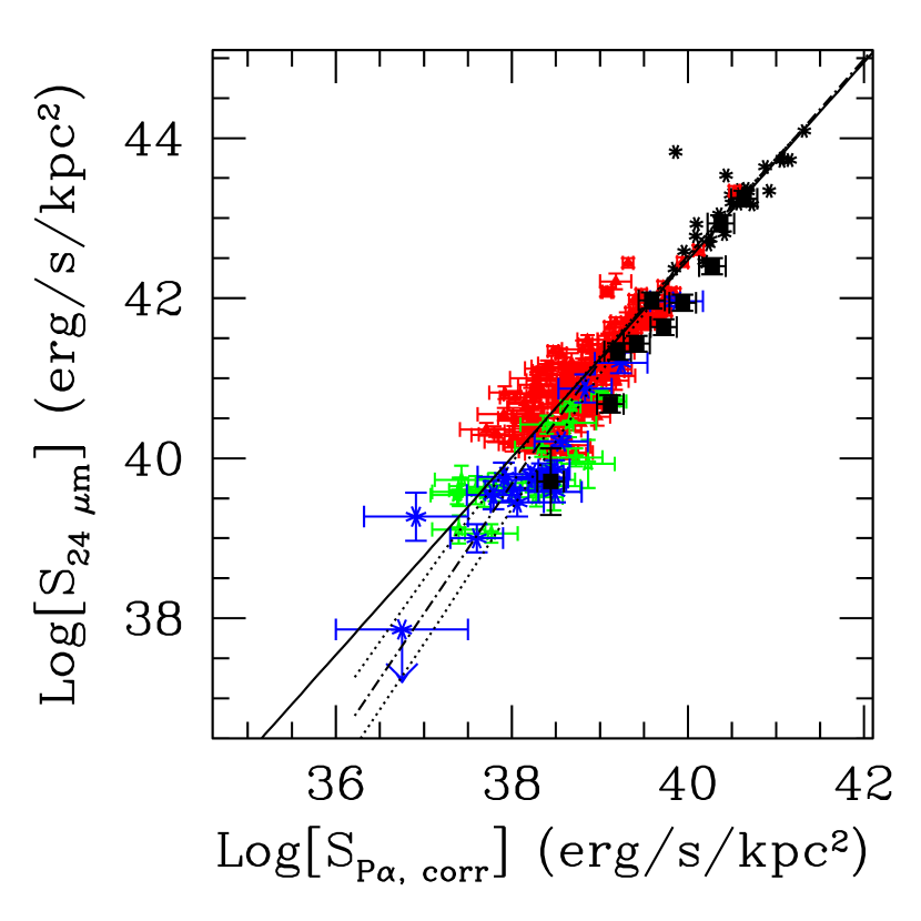
Figure 14: The 24 $\mu$m LSD as a function of Pa$\alpha$ together with the best fit line (continuous straight line, Figure 4). Left. The fiducial model of a dusty 4 Myr old stellar cluster with increasing mass (dot-dashed line) is bracketed by the dispersion curves derived from including in equation A1 the 90 percentile region of the E(B$-$V)–versus–S_Paα,corr correlation (dotted lines and Figure 12). Right Model lines for a 4 Myr old stellar cluster of increasing mass, and two assumptions for the dust distribution that are different from our baseline model: (1) foreground dust geometry and constant E(B$-$V)=1 as a function of S_Paα,corr (short–dash line), and (2) a homogeneously mixed dust–star geometry with no differential extinction between gas and stars, and variable E(B$-$V) according equation A2 (long–dash line).

The 90th percentile region for the E(B$-$V) versus Pa$\alpha$ LSD correlation is shown in Figure 12 by dotted lines that enclose 90% of the data around the mean correlation. The same region is reproduced on the 24 $\mu$m versus Pa$\alpha$ LSDs in Figure 14 (left). We do not show the case for the 8 $\mu$m LSD because the results are similar for both mid–IR bands. The dispersion in the color excess for fixed Pa$\alpha$ LSD has minor impact on our baseline conclusions for the mid–IR emission, with significant impact (factor $\sim$6 peak–to–peak variation) concentrated towards the low–intensity, and low extinction, regions. This effect is readily understood by recalling that once the color excess E(B$-$V)$>$0.5 mag, over 90% of the UV emission is converted by dust into IR emission. Thus, the dependence of E(B$-$V) on the Pa$\alpha$ LSD for S${}_{Pa\alpha,corr}\gtrsim$10³⁹ erg s^-1 kpc^-2 has little impact on the amount of IR emission produced for stellar SEDs that emit most of their power in the UV.

The independence of the IR luminosity on the color excess for high Pa$\alpha$ LSDs is also shown for the case where E(B$-$V) is independent of S_Paα,corr (i.e., equations A2–A4 are not applied). As a simplified example of E(B$-$V) independent of S_Paα,corr, Figure 14 (right) shows the case of constant value E(B$-$V)=1 for all Pa$\alpha$ LSDs. As long as the color excess is sufficiently large that most of the UV stellar light is attenuated by dust, the model’s trend for high luminosity regions does not change. However, when extended to low LSDs, the model with constant E(B$-V$) tends to exceed the low metallicity datapoints, and to show a flatter slope than the best fit line through the high–metallicity data. The latter is due to the models having reached the single photon heating for the 24 $\mu$m emission, where there is a linear correlation between S${}_{24~{}\mu m}$ and S_Paα,corr.

Age variations among different regions have been discussed in section 7, and they effectively account for the spread around the mean trend for the infrared–versus–Pa$\alpha$ LSDs (Figures 9–11). Here we discuss the effect of adopting different dust models than our default one.

Most non–foreground dust geometries, e.g., mixtures of dust and gas/stars, will have the effect of ‘hiding’ from direct detection a proportionally larger fraction of the stellar emission than foreground geometries, thus increasing the observed infrared emission, and S_24μm and S${}_{8\mu m,\ dust}$, relative to the ionizing photon rate (S_Paα,corr) that can be recovered with simple extinction correction methods (e.g., from H$\alpha$/Pa$\alpha$). Figure 14 (right) shows the effect of replacing our foreground dust assumption with an homogeneously mixed dust/stars geometry. The new model follows closely our baseline model up to LSDs S${}_{Pa\alpha,corr}\sim$3$\times$10³⁹ erg s^-1 kpc^-2, and deviates upward of the baseline model for higher LSDs. This is the regime where the dust opacity is such that our standard procedure does not recover completely the number of ionizing photons and S_Paα,corr is underestimated. If we were to allow for dusty cores with arbitrarily high attenuation values in our HII knots, the mixed model would deviate from the baseline model at arbitrarily low Pa$\alpha$ LSDs, thus at least partially accounting for the dispersion of the datapoints around the mean trend.

The competition of the dust with the gas for absorption of the ionizing photons will become increasingly more effective as the density of the star forming regions increases, as in the case of LIRGs and brighter infrared galaxies. Rigby & Rieke (2004) proposes that the lack of high excitation infrared fine structure lines in infrared galaxies is due to much of the massive star formation occurring in ultracompact HII regions, where such competition would be significant. Dopita et al. (2006) have modeled the behavior of such regions, confirming that the infrared continuum should get warmer, but also show the potential to suppress the emission lines substantially.

One of the main assumptions in our analysis is that the ‘typical’ HII knot in our sample is described by a single mean stellar population. Realistically, variations are expected, not only from galaxy to galaxy, but also from region to region. Under most circumstances, each of our apertures will include multiple stellar populations covering a range of ages (Calzetti et al., 2005). Furthermore, the dust covering factor may change from population to population within each region, with older stellar populations often located in areas of lower extinction, or located further away from the dust they heat. The ratio of the 24 $\mu$m LSD to the observed H$\alpha$ LSD, which by construction exacerbates any effect of dust extinction (Figure 15) can provide insights into this effect. The ratio 24 $\mu$m/H$\alpha_{obs}$ spans more than two orders of magnitude for our data, with values between $\sim$0.04 and $\sim$10. The S_24μm/S_Hα,obs ratio is correlated (with a 7 $\sigma$ significance for a Spearman non–parametric test) with the Pa$\alpha$ LSD, with slope $0.83\pm 0.03$ in a log–log plane. This is a different way of expressing the correlation between star formation and dust extinction already shown in Figure 12.

The model lines for solar metallicity are within the general locus of the data–points at low values of the Pa$\alpha$ LSD, especially when the 90–percentile region from Figure 12 is included (Figure 15). The brightest regions in Pa$\alpha$ LSD, and most of the LIRGs, tend to be more consistent with a model where stars and dust are homogeneously mixed and there is no differential extinction between gas and stars (as assumed in all our baseline models, from Calzetti, Kinney & Storchi–Bergmann, 1994). This is not unexpected, as strongly star forming regions are in general more heavily enshrouded in dust than less active regions (Goldader et al., 2002). In addition, in this regime, small errors in the measurement of the (faint) H$\alpha$ line can produce large deviations of the data. The moderate discrepancy between the baseline models and data at the high luminosity end seen in Figure 15 has negligible impact on our results for the mid–IR LSDs as a function of the Pa$\alpha$ LSD (section 6): in this regime, over 80% of the UV light is re-processed by dust into the infrared, and large fluctuations on the stellar light observed directly (including the nebular hydrogen lines) produce only small changes of L(IR).

Despite the potential shortcomings of our assumptions, the ability of the models to describe the overall trends of the data enables us to dissect the individual ‘ingredients’ that produce the observed correlations to better understand their origin.

Table 1: Characteristics of the Sample Galaxies.

Name	Morph.	Nucleus	vH	E(B$-$V)G	Dist.	MV	12$+$log(O/H)	# Regions	HST ID
			(km s-1)		(Mpc)
High Metallicity Galaxies
NGC0925	SAB(s)d		553	0.081	9.12	$-$20.33	8.24–8.78	10	7919, 9360
NGC1512	SB(r)ab		898	0.011	10.5	$-$19.90	8.37–9.05	3	9360
NGC2403	SAB(s)cd		131	0.043	3.5	$-$19.68	8.31–8.81	8	7919
NGC2841	SA(r)b	Sy1/LIN	638	0.017	9.8	$-$21.12	8.52–9.19	5	7919
NGC2976	SAc		3	0.074	3.5	$-$17.97	8.30–8.98	8	7919
NGC3184	SAB(rs)cd		592	0.018	11.10	$-$20.46	8.48–9.14	6	9360
NGC3198	SB(rs)c		663	0.013	13.68	$-$20.90	8.32–8.87	9	9360
NGC3351	SB(r)b		778	0.030	10.1	$-$20.48	8.60–9.22	2	9360
NGC3627	SAB(s)b	Sy2/LIN	727	0.035	8.7	$-$21.17	8.49–9.10	6	7919
NGC3938	SA(s)c		809	0.023	12.2	$-$20.10	8.35–9.07	9	9360
NGC4125	E6	LIN	1356	0.020	21.4	$-$21.89	8.58–9.21	1	9360
NGC4559	SAB(rs)cd		816	0.019	11.1	$-$20.84	8.25–8.79	6	7919
NGC4569	SAB(rs)ab	Sy/LIN	$-$235	0.049	16.58	$-$21.90	8.56–9.19	5	9360
NGC4625	SAB(rs)m		609	0.019	9.17	$-$17.53	8.27–9.04	6	9360
NGC4736	(R)SA(r)ab	Sy2	308	0.019	5.3	$-$20.59	8.31–9.01	5	9360
NGC4826	(R)SA(rs)ab	Sy2	408	0.044	5.6	$-$20.63	8.59–9.24	8	9360
NGC5033	SA(s)c	Sy1.9	875	0.012	13.28	$-$20.87	8.27–8.90	9	9360
NGC5055	SA(rs)bc	LIN	504	0.019	7.82	$-$21.08	8.42–9.13	9	9360
NGC5194	SA(s)bc	Sy2.5	463	0.037	8.2	$-$21.43	8.54–9.18	43	7237
NGC5195	SB0_1	LIN	465	0.038	8.2	$-$19.99	8.28–8.83	1	9360
NGC5866	S0_3	LIN	672	0.014	12.1	$-$20.52	8.43–9.02	3	9360
NGC6946	SAB(rs)cd		48	0.365	5.0	$-$21.11	8.40–9.04	9	9360
NGC7331	SA(s)b	LIN	816	0.097	15.1	$-$22.14	8.40–9.05	8	9360
Medium Metallicity Galaxies
NGC1705	SA0-		632	0.009	5.1	$-$16.29	8.20–8.43	3	7919
IC2574	SAB(s)m		57	0.039	2.8	$-$17.33	7.94–8.26	6	9360
NGC4236	SB(s)dm		0	0.015	4.45	$-$19.12	8.07–8.56	3	9360
IC4710	SB(s)m		739	0.095	7.8	$-$17.96	8.11–8.62	7	7919
NGC6822	IB(s)m		$-$57	0.253	0.47	$-$14.97	8.04–8.67	3	7919
Low Metallicity Galaxies
Ho II	Im		142	0.035	3.5	$-$17.25	7.68–8.07	3	9360
DDO053	Im		20	0.040	3.56	$-$13.68	7.77–8.13	6	9360
Ho IX	Im		46	0.085	3.3	$-$13.67	7.61–7.98	3	9360
M81DwB	Im		347	0.085	6.5	$-$14.20	7.85–8.20	4	9360
NGC5408	IB(s)m		506	0.074	4.8	$-$17.22	7.81–8.23	3	9360
Discarded Galaxies
NGC0024	SA(s)c		554	0.021	8.8	$-$19.01	8.32–8.92	$\cdots$	9360
NGC1291	(R_1)SB(l)0/a		839	0.014	10.5	$-$21.69	8.42–9.01	$\cdots$	9360
M81DwA	I ?		113	0.022	3.55	$\cdots$	7.34–7.64	$\cdots$	9360
NGC3034	I0		203	0.170	5.2	$-$20.51	8.36–9.09	$\cdots$	7919
NGC4631	SB(s)d		606	0.018	8.5	$-$21.59	8.13–8.76	$\cdots$	9360
DDO154	IB(s)m		374	0.010	4.3	$-$14.73	7.54–8.02	$\cdots$	9360

Table 2: Galaxies Measurements.

Name	log SPaα,corr	log SHα,obs	[NII]/H$\alpha$	AV	log S${}_{8\mu m,\ dust}$	log S24μm
	(erg s-1 kpc-2)	(erg s-1 kpc-2)		(mag)	(erg s-1 kpc-2)	(erg s-1 kpc-2)
High Metallicity Galaxies
NGC0925	38.44$\pm$0.18	39.18$\pm$0.08	0.24	0.45$\pm$0.19	41.02$\pm$0.11	40.48$\pm$0.11
NGC1512	38.55$\pm$0.06	38.80$\pm$0.02	0.47	1.94$\pm$0.06	41.09$\pm$0.06	40.75$\pm$0.06
NGC2403	38.73$\pm$0.15	39.27$\pm$0.08	0.62	1.07$\pm$0.17	41.24$\pm$0.11	40.35$\pm$0.11
NGC2841	37.83$\pm$0.30	38.03$\pm$0.30	0.55A	2.12$\pm$0.43	40.43$\pm$0.08	40.08$\pm$0.08
NGC2976	38.50$\pm$0.15	39.12$\pm$0.08	0.30	0.83$\pm$0.17	41.12$\pm$0.10	40.59$\pm$0.10
NGC3184	38.59$\pm$0.18	38.72$\pm$0.11	0.44	2.31$\pm$0.21	40.97$\pm$0.11	40.69$\pm$0.11
NGC3198	38.56$\pm$0.18	38.42$\pm$0.08	0.36	3.16$\pm$0.19	41.20$\pm$0.10	41.09$\pm$0.10
NGC3351	39.24$\pm$0.06	39.48$\pm$0.04	0.40	1.97$\pm$0.07	41.72$\pm$0.06	41.68$\pm$0.06
NGC3627	38.92$\pm$0.23	39.18$\pm$0.04	0.55A	1.94$\pm$0.23	41.72$\pm$0.11	41.33$\pm$0.11
NGC3938	37.99$\pm$0.30	38.76$\pm$0.06	0.54	0.38$\pm$0.31	41.08$\pm$0.08	40.46$\pm$0.08
NGC4125	37.13U	36.00U	$\cdots$	$\cdots$	40.15$\pm$0.06	39.95$\pm$0.06
NGC4559	38.51$\pm$0.30	39.33$\pm$0.08	0.32	0.24$\pm$0.31	41.30$\pm$0.08	40.75$\pm$0.08
NGC4569	38.29$\pm$0.30	38.84$\pm$0.04	0.50A	1.05$\pm$0.30	41.56$\pm$0.08	41.35$\pm$0.08
NGC4625	38.06$\pm$0.11	38.95$\pm$0.08	0.46	0.03$\pm$0.14	40.79$\pm$0.08	40.39$\pm$0.07
NGC4736	37.96$\pm$0.18	38.88$\pm$0.04	0.50	0.01$\pm$0.18	41.96$\pm$0.08	41.54$\pm$0.08
NGC4826	39.28$\pm$0.06	39.53$\pm$0.02	0.55	1.97$\pm$0.06	42.12$\pm$0.06	41.69$\pm$0.06
NGC5033	38.57$\pm$0.08 $\cdots$	$\cdots$	$\cdots$	41.88$\pm$0.06	41.35$\pm$0.06
NGC5055	38.61$\pm$0.11	39.28$\pm$0.08	0.50	0.68$\pm$0.14	41.74$\pm$0.06	41.17$\pm$0.06
NGC5194	38.95$\pm$0.06	39.26$\pm$0.04	0.50	1.78$\pm$0.07	41.54$\pm$0.06	41.19$\pm$0.06
NGC5195	36.89U	37.83U	$\cdots$	$\cdots$	42.39$\pm$0.06	41.35$\pm$0.06
NGC5866	37.64$\pm$0.30	38.19$\pm$0.11	0.55A	1.04$\pm$0.32	40.04$\pm$0.06	39.47$\pm$0.06
NGC6946	39.44$\pm$0.06	39.77$\pm$0.04	0.56	1.72$\pm$0.07	42.34$\pm$0.06	42.20$\pm$0.06
NGC7331	39.08$\pm$0.11	39.14$\pm$0.08	0.32	2.54$\pm$0.14	41.69$\pm$0.08	41.20$\pm$0.08
Medium Metallicity Galaxies
NGC1705	38.56$\pm$0.11	39.48$\pm$0.11	0.09	0.03$\pm$0.16	40.09$\pm$0.06	40.06$\pm$0.06
IC2574	37.55$\pm$0.30	38.44$\pm$0.08	0.12	0.14$\pm$0.31	39.17$\pm$0.18	39.18$\pm$0.18
NGC4236	37.57$\pm$0.30	38.15$\pm$0.08	0.17	1.09$\pm$0.31	39.76$\pm$0.18	39.42$\pm$0.18
IC4710	37.81$\pm$0.30	38.56$\pm$0.08	$\cdots$	0.57$\pm$0.31	39.64$\pm$0.11	39.10$\pm$0.11
NGC6822	37.85$\pm$0.30	38.74$\pm$0.11	$\cdots$	0.12$\pm$0.32	39.46$\pm$0.30	39.13$\pm$0.30
Low Metallicity Galaxies
Ho II	38.37$\pm$0.30	39.31$\pm$0.04	0.10A	0.01$\pm$0.30	40.01$\pm$0.13	40.06$\pm$0.13
DDO053	37.97$\pm$0.30	38.91$\pm$0.11	0.04	0.01$\pm$0.32	39.33$\pm$0.18	39.82$\pm$0.18
Ho IX	36.12$\pm$0.73	36.32$\pm$0.2	0.05A	$\cdots$	36.92U	38.14$\pm$0.30
M81DwB	37.76$\pm$0.18	38.60$\pm$0.08	0.04	0.29$\pm$0.19	39.03$\pm$0.11	39.15$\pm$0.11
NGC5408	38.26$\pm$0.30	39.20$\pm$0.04	0.02	0.01$\pm$0.30	39.29$\pm$0.06	40.05$\pm$0.06

Table 3: Characteristics of the Starburst Galaxies.

Name	Morph.	vH	E(B$-$V)G	R	12$+$log(O/H)
		(km s-1)		(arcsec)
UGCA292	ImIV-V	308	0.016	5.1	7.2
SBS0335$-$052	BCG	4043	0.047	4.1	7.3
HS0822$+$3542	BCG	732	0.047	4.1	7.4
VIIZw403	Pec.	$-$103	0.036	6.1	7.7
UM461	BCD/Irr	1039	0.018	5.1	7.8
Mrk1450	Comp.	946	0.011	5.1	8.0
IIZW40	BCD	789	0.820	11.2	8.1
NGC5253	Im pec	407	0.056	14.2	8.2
NGC2537	SB(s)m	431	0.054	8.1	8.7
NGC2146	SB(a)ab	893	0.096	13.8	8.4–9.0

Table 4: Measurements of the Starburst Galaxies.

Name	log SPaα	log S${}_{8\mu m,\ dust}$	log S24μm
	(erg s-1 kpc-2)	(erg s-1 kpc-2)	(erg s-1 kpc-2)
UGCA292	38.44	40.11$\pm$0.33	39.71$\pm$0.42
SBS0335$-$052	39.59	41.67$\pm$0.02	41.97$\pm$0.10
HS0822$+$3542	39.12	39.48 $\pm$0.21	40.68$\pm$0.11
VIIZw403	39.2	40.48$\pm$0.24	41.34$\pm$0.11
UM461	39.42	40.57$\pm$0.09	41.43 $\pm$0.10
Mrk1450	39.72	40.73$\pm$0.09	41.64$\pm$0.10
IIZw40	40.28	41.59$\pm$0.05	42.4$\pm$0.10
NGC5253	40.37	42.34$\pm$0.07	42.93$\pm$0.10
NGC2537	39.94	42.02$\pm$0.16	41.94$\pm$0.10
NGC2146	40.64	43.44$\pm$0.03	43.24$\pm$0.10

Figure 12: The color excess E(B$-$V), measured from the H$\alpha$/Pa$\alpha$ ratio (section 3.2), as a function of the Pa$\alpha$ LSD, for the 164 HII knots in the high metallicity subsample. The best bi-linear fit through the data (continuous line) has slope $0.61$ (equation A2). The dotted lines mark the region containing 90% of the datapoints around the best fit line. The dash line is from equation A3, where the slope is kept at the fixed value 0.64 (from the Schmidt Law in NGC5194, Kennicutt et al., 2007a).

References

- Allamandola, Tielens & Barker (1985) Allamandola, L.J., Tielens, A.G.G.M., & Barker, J.R. 1985, ApJ, 290, L25
- Allende Prieto et al. (2001) Allende Prieto, C., Lambert, D.L. & Asplund, M. 2001, ApJ, 556, L63
- Alonso–Herrero et al. (2006) Alonso–Herrero, A., Rieke, G.H., Rieke, M.J., Colina, L., Perez-Gonzalez, P.G., & Ryder, S.D. 2006, ApJ, 650, 835
- Barger et al. (1998) Barger, A.J., Cowie, L.L., Sanders, D.B., Fulton, E., Taniguchi, Y., Sato, Y., Kawara, K., & Okuda, H. 1998, Nature, 394, 248
- Bell (2003) Bell, E.F. 2003, ApJ, 586, 794
- Bendo et al. (2006) Bendo, G.J., Dale, D.A., Draine, B.T., Engelbracht, C.W., Kennicutt, R.C., Calzetti, D., Gordon, K.D., Helou, G., Hollenbach, D., Li, AIgen, Murphy, E.J., et al. 2006, ApJ, 652, 283
- Bohlin, Savage & Drake (1978) Bohlin, R.C., Savage, B.D., & Drake, J.F. 1978, ApJ, 224, 132
- Boissier et al. (2004) Boissier, S., Boselli, A., Buat, V., Donas, J., & Milliard, B. 2004, A&A, 424, 465
- Böker et al. (1999) Böker, T., Calzetti, D., Sparks, W., Axon, D., Bergeron, L.E., Bushouse, H., Colina, L., Daou, D., Gilmore, D., Holfeltz, S., et al. 1999, ApJS, 124, 95
- Boselli, Lequeux & Gavazzi (2004) Boselli, A., Lequeux, J., & Gavazzi, G. 2004, A&A, 428, 409
- Bouchet et al. (1985) Bouchet, P., Lequeux, J., Maurice, E., Prevot, L., & Prevot-Burnichon, M. L. 1985, A&A, 149, 330
- Boulanger et al. (1988) Boulanger, F., Beichmann, C., Desert, F.–X., Helou, G., Perault, M., & Ryter, C. 1988, ApJ, 332, 328
- Boulanger et al. (1990) Boulanger, F., Falgarone, E., Puget, J.L., & Helou, G. 1990, ApJ, 364, 136
- Buat et al. (2002) Buat, V., Boselli, A., Gavazzi, G., & Bonfanti, C. 2002, A&A, 383, 801
- Buat et al. (2005) Buat, V., Iglesias-Paramo, J., Seiber, M., Burgarella, D., Charlot, S., Martin, D.C., Xu, C.K., Heckman, T.M.,, Boissier, S., Boselli, A., et al. 2005, ApJ, 619, L51
- Calzetti (2001) Calzetti, D. 2001, PASP, 113, 1449
- Calzetti et al. (2000) Calzetti, D., Armus, L., Bohlin, R.C., Kinney, A.L., Koornneef, J., & Storchi-Bergmann, T. 2000, ApJ, 533, 682
- Calzetti et al. (2005) Calzetti, D., Kennicutt, R.C., Bianchi, L., Thilker, D.A., Dale, D.A., Engelbracht, C.W., Leitherer, C., Meyer, M.J., et al. 2005, ApJ, 633, 871
- Calzetti, Kinney & Storchi–Bergmann (1994) Calzetti, D., Kinney, A.L., & Storchi–Bergmann, T. 1994, ApJ, 429, 582
- Calzetti, Kinney & Storchi–Bergmann (1996) Calzetti, D., Kinney, A.L., & Storchi–Bergmann, T. 1996, ApJ, 458, 132
- Cardelli, Clayton & Mathis (1989) Cardelli, J.A., Clayton, G.C., & Mathis, J.S. 1989, ApJ, 345, 245
- Chapman et al. (2005) Chapman, S.C., Blain, A.W., Smail, I. & Ivison, R.J. 2005, ApJ, 622, 772
- Daddi et al. (2005) Daddi, E., Dickinson, M., Chary, R., Pope, A., Morrison, G., Alexander, D.M., Bauer, F.E., Brandt, W.N., Giavalisco, M., Ferguson, H., Lee, K.-S., Lehmer, B.D., Papovich, C., & Renzini, A. 2005, ApJ, 631, L13
- Dale & Helou (2002) Dale, D.A., & Helou, G. 2002, ApJ, 576, 159
- Dale et al. (2001) Dale, D.A., Helou, G., Contursi, A., Silbermann, N.A., & Kolhatkar, S. 2001, ApJ, 549, 215
- Dale et al. (2006) Dale, D.A., Gil de Paz, A., Gordon, K.D., Armus, L., Bendo, G.J., Bianchi, L., Boissier, S., Calzetti, D., Engelbracht, C.W., Hanson, H.M., Helou, G., Kennicutt, R.C., et al. 2006, ApJ, in press
- Desert, Boulanger & Puget (1990) Desert, F.–X., Boulanger, F., & Puget, J.L. 1990, A&A, 237, 215
- De Vaucouleurs et al. (1991) De Vaucouleurs, G., De Vaucouleurs, A., Corwin, Jr. H.G., Buta, R.J., Paturel, G., & Fouque, P. 1991, Third Reference Cataloguie of Bright Galaxies, Version 3.9
- Devereux & Young (1990) Devereux, N.A., & Young, J.S. 1990, ApJ, 350, L25
- Dopita et al. (2006) Dopita, M. A., Fischera, J.,. Crowley, O., Sutherland, R. S., Christiansen, J., Tuffs, T. J., Popescu, C. C., Groves, B. A., & Kewley, L. J. 2006, ApJ, 639, 788
- Draine & Li (2006) Draine, B.T., & Li A. 2007, ApJ, 657, 810.
- Draine et al. (2007) Draine, B.T., Dale, D.A., Bendo, G., Gordon, K.D., Smith, J.D.T., Armus, L., Engelbracht, C.W., Helou, G., Kennicutt, R.C., Li, A., et al. 2007, ApJ, accepted (astroph/073213).
- Dwek (2004) Dwek E. (astro-ph/0412344)
- Eales et al. (1999) Eales, S., Lilly, S., Gear, W., Dunne, L., Bond, J.R., Hammer, F., Le Fevre, O., & Crampton, D. 1999, ApJ, 515, 518
- Engelbracht et al. (2005) Engelbracht, C.W., Gordon, K.D., Rieke, G.H., Werner, M.W., Dale, D.A., & Latter, W.B. 2005, ApJ, 628, 29
- Engelbracht et al. (2006) Engelbracht, C.W., Kundurthy, P., Gordon, K.D., Rieke, G.H., Kennicutt, R.C., Smith, J.-D. T., Regan, M.W., Makovoz, D., Sosey, M., Draine, B.T., et al. 2006, ApJ, 642, L127
- Engelbracht et al. (2007) Engelbracht, C.W., et al. 2007, in preparation
- Fang et al. (2004) Fang, F. Shupe, D.L., Wilson, G., Lacy, M., Fadda, D., Jarrett, T., Masci, F., Appleton, P.N., Armus, L., Chapman, S., Choi, P.I., et al. 2004, ApJS, 154, 35
- Fitzpatrick (1986) Fitzpatrick, E.L. 1986, AJ, 92, 1068
- Ford et al. (1985) Ford, H.C., Crane, P.C., Jacoby, G.H., Lawrie, D.G., & van der Hulst, J.M. 1985, ApJ, 293, 132
- Förster Schreiber et al. (2004) Förster Schreiber, N.M., Roussel, H., Sauvage, M., & Charmandaris, V., 2004, A&A, 419, 501
- Galliano et al. (2005) Galliano, F., Madden, S.C., Jones, A.P., Wilson, C.D., & Bernard, J.-P. 2005, A&A, 434, 867
- Garnett, Kennicutt & Bresolin (2004) Garnett, D.R., Kennicutt, R.C., & Bresolin, F. 2004, ApJ, 607, L21
- Giavalisco et al. (2004) Giavalisco, M., Dickinson, M., Ferguson, H.C., Ravindranath, S., Kretchmer, C., Moustakas, L.A., Madau, P., Fall, S.M. Gardner, J.P., et al. 2004, ApJ, 600, L103
- Giovanelli et al. (1995) Giovanelli, R., Haynes, M.P., Salzer, J.J., Wegner, G., da Costa, L.N., & Freudling, W., 995, AJ, 110, 1059
- Goad & Gallagher (1985) Goad, J.W., & gallagher, J.S., III 1985, ApJ, 297, 98
- Goldader et al. (2002) Goldader, J.D., Meurer, G,, Heckman, T.M., Seibert, M., Sanders, D.B., Calzetti, D., & Steidel, C.C. 2002, ApJ, 568, 651
- Gordon & Clayton (1998) Gordon, K.D., & Clayton, G.C., 1998, ApJ, 500, 816
- Gordon et al. (2003) Gordon, K.D., Clayton, G.C., Misselt, K.A., Landolt, A.U., & Wolff, M.J. 2003, ApJ, 594, 279
- Gordon et al. (2004) Gordon, K.D., Perez–Gonzalez, P.G., Misselt, K.A., Murphy, E.J., Bendo, G.J., Walfer, F., Thornely, M.D., Kennicutt, R.C., et al. 2004, ApJS154, 215
- Gordon et al. (2005) Gordon, K.D., Rieke, G.H., Engelbracht, C.W., Muzerolle, J., Stanberry, J.A., Misselt, K.A., Morrison, J.E., Cadien, J., et al., 2005, PASP, in press (astroph/0502080)
- Haas, Klaas & Bianchi (2002) Haas, M., Klaas, U., & Bianchi, S. 2002, A&A, 385, L23
- Heckman (1999) Heckman, T.M. 1999, in After the Dark Ages: When Galaxies were Young, S. Holt & E. Smith eds., AIPC 470, 322
- Heckman (2005) Heckman, T.M. 2005, in Starbursts: from 30 Doradus to Lyman Break Galaxies, R. de Grjis & R.M. Gonzalez Delgado eds., in press (astroph/0502022)
- Heckman et al. (1998) Heckman, T.M., Robert, C., Leitherer, C., Garnett, D.R., & van der Rydt, F. 1998, ApJ, 503, 646
- Helfer et al. (2003) Helfer, T.T., Thornley, M.D., Regan, M.W., Wong, T., Sheth, K., Vogel, S.N., Blitz, L., & Bock, D.C.-J. 2003, ApJS145 259
- Helou (1986) Helou, G. 1986, ApJ, 311, L33
- Helou (2000) Helou, G. 2000, in Infrared Astronomy: Today and Tomorrow, eds. F. Casoli, J. Leuquex, & F. David (Springer=–Verlag: Les Ulis), 337
- Helou et al. (1988) Helou, G., Khan, I.R., Malek, L., & Boehmer, L. 1988, ApJS, 68, 151
- Helou, Ryter & Soifer (1991) Helou, G., Ryter, C., & Soifer, B.T. 1991, ApJ. 376, 505
- Helou et al. (2004) Helou, G., Roussel, H., Appleton, P., Frayer, D., Stolovy, S., Storrie–Lombardi, L., Hurst, R., Lowrance, P., et al. 2004, ApJS, 154, 253
- Hill et al. (1997) Hill, J.K., Waller, W.H., Cornett, R.H., Bohlin, R.C., Cheng, K.–P., Neff, S.G., O’Connell, R.W., Roberts, M.S. et al. 1997, ApJ, 477, 673
- Hinz et al. (2005) Hinz, J.C., et al. 2005, in prep.
- Ho, Filippenko & Sargent (1997) Ho, L.C., Filippenko, A.V., & Sargent, W.L.W. 1997, ApJS, 112, 315
- Hogg et al. (2005) Hogg, D.W., Tremonti, C.A., Blanton, M.R., Finkbeiner, D.P., Padmanabhan, N., Quintero, A.D., Schlegel, D., & Wherry, N. 2005, ApJ, 624, 162
- Hoopes & Walterbos (2003) Hoopes, C.G., & Walterbos, R.A.M. 2003, ApJ, 586, 902
- Hopkins (2004) Hopkins, A.M. 2004, ApJ, 615, 209
- Hopkins et al. (2001) Hopkins, A.M., Connolly, A.J., Haarsma, D.B., & Cram, L.E. 2001, AJ, 122, 288
- Houck et al. (2004) Houck, J.R., Charmandaris, V., Brandl, B.R., Weedman, D., Herter, T., Armus, L., Soifer, B.T., Bernard-Salas, J., Spoon, H.W.W., Devost, D., & Uchida, K.I. 2004, ApJS, 154, 211
- Hughes et al. (1998) Hughes, D.H., Serjeant, S., Dunlop, J., Rowan-Robinson, M., Blain, A., Mann, R.G., Ivison, R. Peacock, J., Efstathiou, A., Gear, W., et al. 1998, Nature, 394, 241
- Jarrett (2006) Jarrett, T. 2006, IRAC Extended Source Calibration, http://ssc.spitzer.caltech.edu/irac/calib/extcal/
- Kauffmann et al. (2003) Kauffmann, G., Heckman, T.M., White, S.M., Charlot, S., Tremonti, C., Brinchmann, J., Bruzual, G., Peng, E.W., et al. 2003, MNRAS, 341, 33
- Kennicutt (1998a) Kennicutt, R.C. Jr. 1998a, ARA&A, 36, 189
- Kennicutt (1998b) Kennicutt, R.C. Jr. 1998b, ApJ, 498, 541
- Kennicutt et al. (2007a) Kennicutt, R.C., Calzetti, D. et al. 2007a, ApJ, submitted
- Kennicutt et al. (2007b) Kennicutt, R.C., et al. 2007b, in prep.
- Kennicutt et al. (2003) Kennicutt, R.C., Armus, L., Bendo, G., Calzetti, D., Dale, D.A., Draine, B.T., Engelbracht, C.W., Gordon, D.A., et al. 2003a, PASP, 115, 928
- Kennicutt, Edgar & Hodge (1989) Kennicutt , R.C. Jr., Edgar, B.K., & Hodge, P.W. 1989, ApJ, 337, 761
- Kennicutt & Moustakas (2006) Kennicutt, R.C., & Moustakas, J. 2006, in prep. (SFR in galaxies paper)
- Kewley & Dopita (2002) Kewley, L.J., & Dopita, M.A. 2002, ApJS, 142, 35
- Kewley et al. (2002) Kewley, L.J., Geller, M.J., Jansen, R.A., & Dopita, M.A. 2002, AJ, 124, 3135
- Kobulnicky & Kewley (2004) Kobulnicky, H.A., & Kewley, L.J. 2004, ApJ, 617, 240
- Kong et al. (2004) Kong, X., Charlot, S., Brinchmann, J., & Fall, S.M. 2004, MNRAS, 349, 769
- Koornneef & Code (1981) Koorneef, J., & Code, A.D. 1981, ApJ, 247, 860
- Kroupa (2001) Kroupa, P. 2001, MNRAS, 322, 231
- Laird et al. (2005) Laird, E.S., Nandra, K., Adelberger, K.L., Steidel, C.C., & Reddy, N.A. 2005, MNRAS, 359, 47
- Lamers, Gieles & Portegies Zwart (2005) Lamers, H.J.G.L.M., Gieles, M., & Portegies Zwart, S.F. 2005, A&A, 429, 173
- Landini et al. (1984) Landini, M., Natta, A., Salinari, P., Oliva, E., Moorwood, A.F.M. 1984, A&A, 134, 284
- Leger & Puget (1984) Leger, A., & Puget, J.L. 1984, A&A, 137, L5
- Leitherer et al. (1999) Leitherer, C., Schaerer, D., Goldader, J.D., González Delgado, R.M., Robert, C., Kune, D.F., de Mello, D.F., Devost, D., & Heckman, T.M. 1999, ApJS, 123, 3
- Lequeux et al. (1982) Lequeux, J., Maurice, E., Prevot-Burnichon, M.-L., Prevot, L., & Rocca-Volmerange, B. 1982, A&A, 113, L15
- Li & Draine (2001) Li, A., & Draine, B.T. 2001, ApJ, 554, 778
- Li & Draine (2002) Li, A., & Draine, B.T. 2002, ApJ, 572, 762
- Lonsdale Persson & Helou (1987) Lonsdale Persson, C.J., & Helou, G.X. 1987, ApJ, 314, 513
- Madden et al. (2006) Madden et al. 2006, A&A, 446, 877
- Martin (1997) Martin, C.L., 1997, ApJ, 491, 561
- Masegosa, Moles & Campos–Aguilar (1994) Masegosa, J., Moles, M., & Campos–Aguilar, A. 1994, ApJ, 420, 576
- Masters (2005) Masters, K.L. 2005, Ph. D. Thesis
- Mathis, Mezger & Panagia (1983) Mathis, J.S., Mezger, P.G., & Panagia, N. 1983, ApJ, 128, 212
- Mattioda et al. (2005) Mattioda, A.L., Allamandola, L.J., & Hudgins, D.M. 2005, ApJ, 629, 1183
- Mayya & Prabhu (1996) Mayya, Y.D., & Prabhu, T.P. 1996, AJ, 111, 1252
- Meurer, Heckman & Calzetti (1999) Meurer, G.R., Heckman, T.M., & Calzetti, D. 1999, ApJ, 521, 64
- Moustakas, Kennicutt & Tremonti (2006) Moustakas, J., Kennicutt, R.C., & Tremonti, C.A. 2006, ApJ, 642, 775
- Moustakas et al. (2007) Moustakas, J., Kennicutt, R.C., et al. 2007, in prep.
- Osterbrock & Ferland (2006) Osterbrock, D.E., & Ferland, G.J. 2006, Astrophysics of Gaseous Nebulae and Active Galactic Nuclei, 2nd edition (Sausalito (CA): University Science Books)
- Peeters, Spoon & Tielens (2004) Peeters, E., Spoon, H.W.W., & Tielens, A.G.G.M. 2004, ApJ, 613, 986
- Peletier & Willner (1992) Peletier, R.F., & Willner, S.P. 1992, AJ, 103, 1761
- Perez–Gonzalez et al. (2006) Perez–Gonzalez, P.G., Kennicutt, R.C., Gordon, K.D., Misselt, K.A., Gil de Paz, A., Engelbracht, C.W., Rieke, G.H., Bendo, G.J., Bianchi, L., Boissier, S., Calzetti, D., Dale, D.A., et al. 2006, ApJ, 648, 987
- Pety et al. (2005) Pety, J., Teyssier, D., Fosse‘, D., Gerin, M., Roueff, E., Abergel, A., Habart, E., & Cernicharo, J. 2005, A&A, in press (astroph/0501339)
- Pilyugin (2001) Pilyugin, L.S. 2001, A&A, 374, 412
- Pilyugin & Thuan (2005) Pilyugin, L.S., & Thuan, T.X. 2005, ApJ, 631, 231
- Prescott et al. (2007) Prescott, M., Kennicutt, R.C., et al. 2007, ApJ, submitted.
- Quillen & Yukita (2001) Quillen, A. C., & Yukita, M. 2001, ApJ, 121, 2095
- Reach et al. (2005) Reach, W.T., Megeath, S.T., Cohen, M., Hora, J., Carey, S., Surace, J., Willner, S.P., Barmby, P., Wilson, G., Glaccum, W., Lowrance, P., Marengo, M., & Fazio, G. 2005, PASP117, 978
- Regan et al. (2004) Regan, M.W., Thornley, M.D., Bendo, G.J., Draine, B.T., Li, A., Dale, D.A., Engelbracht, C.W., Kennicutt, R.C., et al. 2004, ApJS, 154, 204
- Rigby & Rieke (2004) Rigby, J. R. & Rieke, G. H. 2004, ApJ, 606, 237
- Rosa–Gonzalez, Terlevich & Terlevich (2002) Rosa–Gonzalez, D., Terlevich, E., & Terlevich, R. 2002, MNRAS, 332, 283
- Rosenberg et al. (2006) Rosenberg, J.L., Ashby, M.L.N., Salzer, J.J., & Huang, J.-S. 2006, ApJ, 636, 742
- Roussel et al. (2001) Roussel, H., Sauvage, M., Vigroux, L., & Bosma, A. 2001, A&A, 372, 427
- Rowan–Robinson & Crawford (1989) Rowan–Robinson, M., & Crawford, J. 1989, MNRAS, 238, 523
- Salim et al. (2007) Salim, S., Rich, M.R., Charlot, S., Brinchmann, J., Johnson, B.D., Schminovich, D., Seibert, M., Mallery, R., Heckman, T.M., Forster, K., et al. 2007, ApJS, in press (astroph/0704.3611)
- Sanders et al. (2003) Sanders, D.B., Mazzarella, J.M., Kim, D.-C., Surace, J.A., & Soifer, B.T. 2003, AJ, 126, 1607
- Sauvage & Thuan (1992) Sauvage, M., & Thuan, T.X. 1992, ApJ, 396, L69
- Schlegel, Finkbeiner & Davis (1998) Schlegel, D.J., Finkbeiner, D.P., & Davis, M. 1998, ApJ, 500, 525
- Sellgren (1984) Sellgren, K. 1984, ApJ, 277, 623
- Sellgren, Luan & Werner (1990) Sellgren, K., Luan, L., & Werner, M.W. 1990, ApJ, 359, 384
- Scoville et al. (2001) Scoville, N.Z., Polletta, M., Ewald, S., Stolovy, S.R., Thompson, R., & Rieke, M. 2001, AJ, 122, 3017
- Sheth et al. (2002) Sheth, K., Vogel, S.N., Regan, M.W., Teuben, P.J., Andrew, I., & Thornley, M.D. 2002, AJ, 124, 2581
- Smail, Ivison & Blain (1997) Smail, I., Ivison, R.J., & Blain, A.W. 1997, ApJ, 490, L5
- Smith et al. (2007) Smith, J.D.T., Draine, B.T., Dale, D.A., Moustakas, J., Kennicutt, R.C., Helou, G., Armus, L., Roussel, H., Seth, K., Bendo, G.J., et al. 2007, ApJ, 656, 770
- Sullivan et al. (2001) Sullivan, M., Mobasher, B., Chan, B., Cram, L., Ellis, R., Treyer, M., & Hopkins, A. 2001, ApJ, 558, 72
- Surace, Sanders & Mazzarella (2004) Surace, J.A., Sanders, D.B., & Mazzarella, J.M. 2004, AJ, 127, 3235
- Tacconi–Garman et al. (2005) Tacconi–Garman, L.E., Sturm, E., Lehnert, M., Lutz, D., Davies, R.I., & Moorwood, A.F.M. 2005, A&A, in press (astroph/0411272)
- van der Hulst et al. (1988) van der Hulst, J.M., Kennicutt, R.C., Crane, P.C., & Rots, A.H. 1988, A&A, 195, 38
- Walter et al. (2007) Walter, F., Cannon, J.M., Roussel, H., Bendo, G.J., Calzetti, D., Dale, D.A., Draine, B.T., Helou, G., Kennicutt, R.C., Brinks, E., de Block, W.J.G., et al. 2007, ApJ, accepted.
- Wang & Heckman (1996) Wang, B., & Heckman, T.M. 1996, ApJ, 457, 645
- Wu et al. (2005) Wu, H., Cao, C., Hao, C.-N., Liu, F.-S., Wang, J.-L., Xia, X.-Y., Deng, Z.-G., & Young, C. K.-S. 2005, ApJ, 632, L79
- Wu et al. (2006) Wu, Y., Charmandaris, V., Hao, L., Brandl, B.R., Bernard-Salas, J., Spoon, H.W.W., & Houck, J.R. 2006, ApJ, 639, 157