JLQCD collaboration and TWQCD collaboration
Two-flavor lattice QCD in the -regime and chiral Random Matrix Theory
Abstract
The low-lying eigenvalue spectrum of the QCD Dirac operator in the -regime is expected to match with that of chiral Random Matrix Theory (ChRMT). We study this correspondence for the case including sea quarks by performing two-flavor QCD simulations on the lattice. Using the overlap fermion formulation, which preserves exact chiral symmetry at finite lattice spacings, we push the sea quark mass down to 3 MeV on a lattice at a lattice spacing 0.11 fm. We compare the low-lying eigenvalue distributions and find a good agreement with the analytical predictions of ChRMT. By matching the lowest-lying eigenvalue we extract the chiral condensate, , where errors represent statistical and higher order effects in the expansion. We also calculate the eigenvalue distributions on the lattices with heavier sea quarks at two lattice spacings. Although the expansion is not applied for those sea quarks, we find a reasonable agreement of the Dirac operator spectrum with ChRMT. The value of , after extrapolating to the chiral limit, is consistent with the estimate in the -regime.
pacs:
11.15.Ha,11.30.Rd,12.38.GcI Introduction
Numerical simulations of QCD on the lattice suffer from various sources of systematic errors, such as finite lattice spacing , finite volume , and larger quark masses than those in the nature. Each of these needs to be eliminated by an extrapolation using several independent simulations. In particular, the extrapolation in the quark mass to the chiral (or physical) limit is non-trivial, because most physical quantities have non-analytic dependence on the quark masses due to pion loop effects as predicted by chiral perturbation theory (ChPT). In order to reproduce such non-analytic behavior, the physical volume must be increased as the chiral limit is approached such that the pion Compton wavelength fits in the box. Therefore, in practice the chiral extrapolation must be done with a limited range of quark masses, which is a potential source of large systematic uncertainty. This becomes more problematic when the chiral symmetry is explicitly violated by the fermion formulation on the lattice, since the standard ChPT cannot be used as a guide in the extrapolation and the chiral extrapolation must be combined with the continuum extrapolation.
An alternative approach is to study the -regime of QCD Gasser:1987ah ; Hansen:1990un ; Hansen:1990yg ; Leutwyler:1992yt on the lattice. In this regime the quark mass is set close to the chiral limit while keeping the physical volume finite. The system suffers from a large finite volume effect, but it can be systematically calculated by ChPT, because the pion field dominates the low energy dynamics of the system and the effects of other heavier hadrons become sub-dominant. It means that the low energy constants appearing in ChPT Lagrangian can be extracted from the lattice calculation in the -regime by comparing with ChPT predictions. Since a small violation of chiral symmetry gives large effects in the -regime, the lattice fermion formulation must fully respect the chiral symmetry.
The -regime is reached by reducing the quark mass , at a finite volume , down to the region where the pion mass satisfies the condition
| (1) |
where denotes the QCD scale. Under the condition (1), the zero momentum modes of the pion field give the dominant contribution since the energy of finite momentum modes is too large to excite. In this way, ChPT is organized as an expansion in terms of the parameter where is the ultraviolet cut-off of ChPT (typically taken to be with the pion decay constant). Since the quantum correction of the zero-modes is not suppressed in the -regime and the path integral over SU() manifold must be explicitly carried out, the partition function and other physical quantities show remarkable sensitivity to the topology of the gauge field.
At the leading order of the -expansion, the partition function of ChPT is equivalent to that of chiral Random Matrix Theory (ChRMT) Shuryak:1992pi ; Smilga:1995nk ; Verbaarschot:2000dy ; Damgaard:2000ah ; Akemann:2006ru at any fixed topological charge. Moreover, from the symmetry of the Dirac operator, the low-lying QCD Dirac spectrum is expected to be in the same universality class of ChRMT. ChRMT thus provides a direct connection between Dirac eigenvalues and the effective theory describing the dynamical chiral symmetry breaking. One of the most convenient predictions of ChRMT is the distribution of individual eigenvalue, which can be directly compared with the lattice data. Such comparison has been done mainly in the quenched approximation Edwards:1999ra ; Bietenholz:2003mi ; Giusti:2003gf ; Wennekers:2005wa , except for a work using the reweighting technique Ogawa:2005jn or for some recent attempts of carrying out dynamical fermion simulation on coarse lattices DeGrand:2006nv ; Lang:2006ab . The eigenvalue spectrum in those calculations shows a good agreement with the prediction of ChRMT as far as the lattice volume is large enough .
In this work we perform lattice QCD simulations in and out of the -regime including two light flavors of dynamical quarks. Since we are interested in the consequences of chiral symmetry breaking, we employ the Neuberger’s overlap-Dirac operator Neuberger:1997fp ; Neuberger:1998wv , which preserves exact chiral symmetry Luscher:1998pq at finite lattice spacings. The exact chiral symmetry is also helpful for numerical simulations in the -regime, because the lowest-lying eigenvalue of the Hermitian overlap-Dirac operator is bounded from below (by a small but finite mass term) and no numerical instability occurs. The space-time volume of our lattice is with the lattice spacing 0.11–0.125 fm. The gauge field topology is fixed to the trivial topological sector by introducing the extra Wilson fermions and ghosts Fukaya:2006vs . We perform the Hybrid Monte Carlo simulation with the sea quark mass around 3 MeV, which corresponds to the -regime: the expected pion Compton wavelength is comparable to the lattice extent . The numerical cost for such a small sea quark mass is very expensive in general, but it is not prohibitive on the small lattice as required in the -regime simulation. We also carry out simulations at several quark masses roughly in the region - with the physical strange quark mass, which are out of the regime.
We study the eigenvalue spectrum of the overlap-Dirac operator on the configurations generated with these dynamical quarks. A good agreement of the low-lying eigenvalue spectrum with ChRMT predictions has already been reported in our earlier paper Fukaya:2007fb for the run in the -regime. The present paper describes our analysis in more detail. Since ChRMT provides the distribution of individual eigenvalues, the test of the agreement can be made using the information on the shape of the distribution, not just using the average values. We find a good agreement of the lowest-lying eigenvalue distribution by analyzing its several moments. If we look at higher eigenvalues, the agreement becomes marginal, because there are contaminations from the bulk of the eigenvalue spectrum corresponding to finite momentum pion states and other higher excited states, which are not described by ChRMT. We study the bulk eigenvalue spectrum and identify the region where the analysis in the -regime is applied.
A direct output from the comparison of the eigenvalue spectrum is the value of chiral condensate . We extract from the lowest-lying eigenvalue in the -regime. For comparison we also calculate it on heavier quark mass lattices and extrapolate them to the chiral limit. Although the leading order relations in the expansion is not valid for these lattices, the result in the chiral limit shows remarkable agreement with the direct calculation in the -regime. We convert the value of obtained on the lattice to the common definition in the continuum renormalization scheme using the non-perturbative renormalization (NPR) technique through the RI/MOM scheme which is a regularization independent scheme based on the Green’s functions of the offshell quark Martinelli:1994ty .
This paper is organized as follows. In Section II, we review ChRMT calculations of the Dirac eigenvalue spectrum. The details of the numerical simulations are described in Section III, and the results of the low-lying modes in the -regime is discussed in Section IV. The low-mode spectrum in the -regime are presented in Section V. In Section VI we also study the higher eigenvalue spectrum. Our conclusions are given in Section VII.
II Chiral Random Matrix Theory
In the -regime the low-lying eigenvalue spectrum of -flavor QCD Dirac operator matches with that of Chiral Random Matrix Theory (ChRMT) Shuryak:1992pi ; Smilga:1995nk ; Verbaarschot:2000dy ; Damgaard:2000ah up to a scale factor as described below. This can be derived by identifying the partition function of ChRMT
| (2) |
with the QCD partition function in the -regime. Since the dependence on the global topology becomes manifest in the -regime, we work in a fixed topological sector . Here, is a complex matrix, and . The parameter plays a role of quark mass. In the limit of large , the partition function (2) can be modified to the form describing the zero-momentum mode of ChPT Shuryak:1992pi
| (3) |
from which one can identify .
The advantage of ChRMT (2) is that the eigenvalue distribution of the matrix is analytically known Damgaard:2000ah . Here we reproduce the known result for the case of two degenerate flavors and zero topological charge, which is relevant in this work.
Let us consider the -th lowest microscopic eigenvalue , with the -th eigenvalue of . The distribution of is written as
| (4) |
where . The form of is analytically known in the microscopic limit, i.e. while is kept fixed:
| (5) |
The matrices and are given by
| (6) |
where and . ’s are the modified Bessel functions.
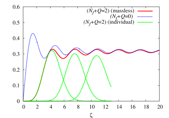
The spectral density is given by a sum of the individual distributions
| (7) |
In the massless and the infinite mass (or quenched) limit, it can be written in a simple form,
| (8) |
where denotes the Bessel functions of the first kind. Their shape and the individual eigenvalue distributions are shown in Figure 1.
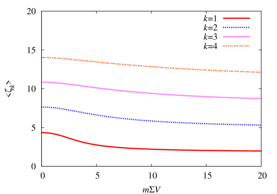
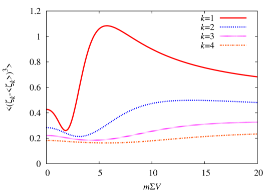
In order to quantify the shape of the distributions, we consider -th moments
| (9) |
which can be calculated numerically. The results for are shown in Figure 2 as a function of . From the plot for one can see that the lowest eigenvalue is lifted near the massless limit due to a repulsive force by the dynamical fermions. When is greater than 10, the eigenvalues qualitatively behave as in the quenched theory (or limit). Transition from the massless two-flavor theory to the quenched theory occurs around 1–10, where the moments of the lowest-lying eigenvalue show rather peculiar dependence on .

The ChRMT spectrum is expected to match with those of the QCD Dirac operator up to a constant . For example, the lowest eigenvalue of the QCD Dirac operator is matched as
| (10) |
from which one can extract , one of the fundamental constant in ChPT. Unlike the standard lattice QCD calculation, we do not need any chiral extrapolation, as is already very small in the -regime. By investigating the consistency with the determination through higher eigenvalues or their shapes, one can estimate possible systematic errors due to higher order effects in the expansion.
III Numerical Simulation
III.1 Overlap fermion implementation
We employ Neuberger’s overlap fermion formulation Neuberger:1997fp ; Neuberger:1998wv for the sea quarks. Its Dirac operator is defined as
| (11) |
where denotes the Hermitian Wilson-Dirac operator with a large negative mass . We choose throughout this work. (Here and in the following the parameters are given in the lattice unit.) The overlap-Dirac operator (11) satisfies the Ginsparg-Wilson relation Ginsparg:1981bj
| (12) |
when the quark mass vanishes. Because of this relation, the fermion action built up with (11) has an exact chiral symmetry under the modified chiral transformation Luscher:1998pq .
In the practical application of the overlap-Dirac operator (11), the profile of near-zero modes of the kernel operator is important, as they determine the numerical cost of the overlap fermion. The presence of such near-zero modes is also a problem for the locality property of the overlap operator Hernandez:1998et . For most gauge actions used in practical simulations, it is known that the spectral density of the operator is non-zero at vanishing eigenvalue = 0 Edwards:1998sh due to the so-called dislocations, i.e. local lumps of the gauge configuration Berruto:2000fx . We avoid this problem by introducing additional fermions and ghosts to generate a weight
| (13) |
in the partition function Fukaya:2006vs . (The same idea is proposed in the context of the domain-wall fermion Izubuchi:2002pq ; Vranas:2006zk .) They are unphysical as their mass is of order of lattice cutoff, and thus does not affect low-energy physics. The numerator suppresses the near-zero modes, while the denominator cancels unwanted effects for higher modes. The “twisted-mass” parameter determines the value of threshold below which the eigenmodes are suppressed. We set = 0.2 in this work. With these extra degrees of freedom, the spectral density vanishes at the vanishing eigenvalue , and the numerical cost of approximating the sign function in (11) is substantially reduced Fukaya:2006vs .
We approximate the sign function using a rational function of the form (see, e.g., vandenEshof:2002ms ; Chiu:2002eh )
| (14) |
where is the lower limit of the range of approximation and . The coefficients , and can be determined analytically (the Zolotarev approximation) so as to optimize the accuracy of the approximation. Since we have to fix the lower limit , we calculate a few lowest-lying eigenvalues and project them out before applying (14) when their absolute value is smaller than . The value of is 0.144 in our simulations. The accuracy of the approximation improves exponentially as the number of poles increases. With , the sign function is approximated to a - level. Since the multi-shift conjugate gradient method can be used to invert all the terms at once, the numerical cost depends on only weakly.
In the -regime the partition function and other physical quantities show striking dependence on the global topological charge of gauge field. With the lattice action including (13) the topological charge never changes during the Hybrid Monte Carlo (HMC) simulations, which consists of molecular dynamics (MD) evolution of gauge field configuration. This is because the topology change must accompany a zero crossing of the eigenvalue of , which is forbidden by the factor (13). The gauge configuration in a fixed topological sector can therefore be effectively sampled. In this work the simulations are restricted in the trivial topological sector except for one quark mass parameter for which we carry out independent simulations at and .
Here, we assume that the ergodicity of the simulation in a fixed topological sector is satisfied even with the determinant (13). In order to confirm this, we are studying the fluctuation of the local topological charge density, which will be reported in a separate paper.
III.2 HMC simulations
We perform two-flavor QCD simulations using the overlap fermion for the sea quarks, with the approximated sign function (14) with . Lattice size is throughout this work. For the gauge part of the action, we use the Iwasaki action Iwasaki:1985we ; Iwasaki:1984cj at = 2.30 and 2.35, which correspond to the lattice spacing = 0.12 fm and 0.11 fm, respectively, when used with the extra Wilson fermions and ghosts. The simulation parameters are listed in Tables 1 and 2 for = 2.30 and 2.35, respectively.
| traj. | [fm] | ||
|---|---|---|---|
| 0.015 | 10,000 | 0 | 0.1194(15) |
| 0.025 | 10,000 | 0 | 0.1206(18) |
| 0.035 | 10,000 | 0 | 0.1215(15) |
| 0.050 | 10,000 | 0 | 0.1236(14) |
| 0.050 | 5,000 | ||
| 0.050 | 5,000 | ||
| 0.070 | 10,000 | 0 | 0.1251(13) |
| 0.100 | 10,000 | 0 | 0.1272(12) |
The configurations from the runs at = 2.30 are for various physics measurements including hadron spectrum, decay constants, form factors, bag parameters, and so on. In this work we use them to analyze the eigenvalue spectrum. The simulation details will be described in a separate paper Kaneko_HMCnf2 , but we reproduce some basic parameters in Table 1. They include the sea quark mass , trajectory length (the unit trajectory length is 0.5 MD time), topological charge and lattice spacing determined from the Sommer scale (= 0.49 fm) Sommer:1993ce of the heavy quark potential. In the massless limit, the lattice spacing is found to be 0.1184(12) fm by a linear extrapolation in . The sea quark mass at = 2.30 covers the region from to with the physical strange quark mass.
| traj. | [fm] | ||||||||
|---|---|---|---|---|---|---|---|---|---|
| 0.002 | 3,690 | 0.2 | 0.0714 | 1/4 | 1/5 | 0.90(23) | 0.756 | 0.62482(1) | 0.1111(24) |
| 1,010 | 0.2 | 0.0625 | 1/4 | 1/5 | 1.24(50) | 0.796 | 0.62479(2) | ||
| 0.020 | 1,200 | 0.2 | 0.0714 | 1/4 | 1/5 | 0.035(09) | 0.902 | 0.62480(1) | 0.1074(30) |
| 0.030 | 1,200 | 0.4 | 0.0714 | 1/4 | 1/5 | 0.253(20) | 0.743 | 0.62480(2) | 0.1127(23) |
| 0.045 | 1,200 | 0.4 | 0.0833 | 1/5 | 1/6 | 0.189(18) | 0.768 | 0.62476(2) | 0.1139(29) |
| 0.065 | 1,200 | 0.4 | 0.1 | 1/5 | 1/6 | 0.098(12) | 0.838 | 0.62474(2) | 0.1175(26) |
| 0.090 | 1,200 | 0.4 | 0.1 | 1/5 | 1/6 | 0.074(19) | 0.855 | 0.62472(2) | 0.1161(24) |
| 0.110 | 1,200 | 0.4 | 0.1 | 1/5 | 1/6 | 0.052(10) | 0.868 | 0.62471(2) | 0.1182(22) |
The runs at = 2.35 were originally intended for a basic parameter search and therefore the trajectory length for each sea quark mass is limited (1,200 HMC trajectories). It is at this value that we performed a run in the -regime by pushing the sea quark mass very close to the chiral limit , which is one order of magnitude smaller than the sea quark mass in other runs. In Table 2 we summarize several simulation parameters. Among them, the basic parameters are the sea quark mass , trajectory length, plaquette expectation value , and lattice spacing. The massless limit of the lattice spacing is evaluated to be 0.1091(23) fm using a linear extrapolation with data above = 0.020. This value is consistent with the result of the -regime run at = 0.002. The other parameters are explained below.
The HMC simulation with the overlap fermion was first attempted by Fodor, Katz and Szabo Fodor:2003bh and soon followed by two other groups DeGrand:2004nq ; Cundy:2005pi . They introduced the so-called reflection-refraction trick in order to treat the discreteness of the HMC Hamiltonian at the topological boundary. This leads to a significant additional cost for dynamical overlap fermions compared to other (chirally non-symmetric) fermion formulations. We avoid such extra costs by introducing the extra Wilson fermion determinants (13), with which the MD evolution never reaches the topological boundary.
In the implementation of the HMC algorithm, we introduce the Hasenbusch’s mass preconditioner Hasenbusch:2001ne together with the multiple time step technique Sexton:1992nu . Namely, we rewrite the fermion determinant as
| (15) |
by introducing a heavier overlap fermion with mass . We then introduce a pseudo-fermion field for each determinant. In the right hand side of (15) the second term is most costly as it requires an inversion of the overlap operator with a small mass . On the other hand, the contribution to the MD force from that term can be made small by tuning close to . With the multiple time step technique, such small contribution does not have to be calculated frequently, while the force from the first term must be calculated more often. We introduce three time steps: (i) for the ratio , (ii) for the preconditioner , and (iii) for the gauge action and the extra Wilson fermions (13). By investigating the size of MD forces from each term, we determine the time steps and the preconditioner mass as listed in Table 2. For the run in the -regime ( = 2.35, = 0.002) we switched to a smaller value in the middle of the run, since we encounter a trajectory which has exceptionally large MD force from the ratio probably due to a small eigenvalue of .
An average shift of Hamiltonian during a unit trajectory determines the acceptance rate in the HMC algorithm. It must be or less to achieve a good acceptance rate, which is satisfied in our runs as listed in Table 2. The value at = 0.002 is larger and around 0.9–1.2. This is due to so-called “spikes” phenomena, i.e. exceptionally large values () of at some trajectories. The spikes are potentially dangerous as they may spoil the exactness of the HMC algorithm, but we believe that this particular run is valid since we have checked that the area preserving condition is satisfied within statistical errors.
For the inversion of the overlap operator we use the relaxed conjugate gradient algorithm Cundy:2004pz . The trick is to relax the convergence condition of the inner solver as the conjugate gradient loop proceeds. This is allowed because the change of the solution vector becomes smaller at the later stages of the conjugate gradient. The gain is about a factor of 2 compared to the conventional conjugate gradient. In the middle of the simulations at = 2.30, we replaced the overlap solver by the one with a five-dimensional implementation Matsufuru:2006xr . This is faster by another factor of 4–5 than the relaxed conjugate gradient method. These details of the algorithm will be discussed in a separate paper Kaneko_HMCnf2 .

The numerical cost depends on how precisely the matrix inversions are calculated. At an inner level there are inversions of the Hermitian Wilson-Dirac operator appearing in the rational approximation (14). The inversions can be done at the same time using the multi-shift conjugate gradient. We calculate until all the solutions reach the relative precision when adopted in the calculation of the HMC Hamiltonian. This value matches the precision we are aiming at for the approximation of the sign function. In the molecular dynamics steps the relative precision is relaxed to . The conjugate gradient for the overlap-Dirac operator at the outer level is also carried out to the level of the () relative precision in the HMC Hamiltonian (MD force) calculation.
The numerical cost can be measured by counting the number of the Wilson-Dirac operator multiplication, although other manipulations, such as the linear algebra of vectors, are not negligible. The number of the Wilson-Dirac operator multiplication is plotted in Figure 3 for the runs at . The upper panel shows the cost per trajectory; the lower panel presents the cost of inverting the overlap-Dirac operator when we calculate the Hamiltonian at the end of each trajectory. The expected mass dependence for the overlap solver is with the lowest-lying eigenvalue of the overlap operator . Therefore, the cost is proportional to only when is much greater than . This condition is satisfied for at and larger than 0.030, where is around 0.004 as we show later. Fitting the data with the scaling law above = 0.030, we obtain the power as 0.82, which is roughly consistent with the expectation. For the total cost of the HMC Hamiltonian (upper panel), the quark mass dependence is more significant, since it depends on the choice of the step sizes. It is not even a smooth function of . If we fit the data with the power law above = 0.030 as in the case of the solver, we obtain = 0.49, which gives a much milder quark mass dependence.
The machine time we spent is roughly one hour per trajectory for the run in the -regime () on a half rack (512 computing nodes) of IBM BlueGene/L. The cost at other mass parameters is lower as one can see in Figure 3. The numerical cost at = 2.30 is higher, because the number of the near-zero modes of is significantly larger.
For comparison we also generated quenched configurations on a lattice at = 2.37 in the topological sector = 0 and 2. We must use the HMC algorithm even for the quenched simulation, as it contains the extra Wilson fermions (13). We accumulated 20,000 trajectories for each topological sector and used the gauge configurations for measurement at every 200 trajectories. The lattice spacing is 0.126(2) fm, which matches the dynamical lattices at in the heavier sea quark mass region = 0.075 and 0.100. In the chiral limit the dynamical lattices are slightly finer.
III.3 Eigenvalue calculation
In the HMC simulations described in the previous section, we stored the gauge configurations at every 10 trajectories for measurements. For those configurations we calculate lowest 50 eigenvalues and eigenvectors of the overlap-Dirac operator . In the analysis of this work we only use the eigenvalues.
We use the implicitly restarted Lanczos algorithm for a chirally projected operator
| (16) |
where . This operator is Hermitian and its eigenvalue gives the real part of the eigenvalue of the original overlap operator . The pair of eigenvalues (and its complex conjugate) of can be obtained from using the relation derived from the Ginsparg-Wilson relation (12).
In the calculation of the eigenvalues we enforce better accuracy in the approximation of the sign function by increasing the number of poles in the rational function. The sign function is then approximated at least to the level. In order to improve the convergence of the Lanczos algorithm we use the Chebyshev acceleration technique Neff:2001zr ; DelDebbio:2005qa and optimize the window of eigenvalues for the target low-lying modes.
For the comparison with ChRMT, the lattice eigenvalue is projected onto the imaginary axis as . Note that is very close to (within 0.05%) for the low-lying modes we are interested in. We consider positive ’s in the following.
In Figure 4 we plot the ensemble averages of the lowest 5 eigenvalues ( = 1–5) as a function of the sea quark mass. The data at = 2.35 are shown. We observe that the low-lying spectrum is lifted as the chiral limit is approached. This is a direct consequence of the fermion determinant , which repels the small eigenvalues from zero when the lowest eigenvalue is larger than . This is exactly the region where the numerical cost saturates as it is controlled by rather than .


Figure 5 shows a Monte Carlo history of the lowest-lying eigenvalue at the lightest ( = 0.002) and the heaviest ( = 0.110) sea quark masses at = 2.35. At = 0.002 we find some long range correlation extending over a few hundred trajectories, while the history = 0.110 seems more random. In order to quantify the effect of autocorrelation we investigate the bin-size dependence of the jackknife error for the average ( = 1–5). As can be seen from Figure 6 the jackknife error saturates around the bin-size 20, which corresponds to 200 HMC trajectories. This coincides with our rough estimate from Figure 5. In the following analysis we take the bin-size to be 20 at = 0.002 and 10 at other sea quark masses.
IV Low-mode spectrum in the -regime
In this section we describe a comparison of the lattice data for the low-lying eigenvalues with the predictions of ChRMT. The most relevant data set in our simulations is the one at = 0.002 and = 2.35, since this is the only run within the -regime.
First we determine the scale, or the chiral condensate, from the first eigenvalue through (10). By solving
| (17) |
recursively in order to correct the dependence of , we obtain and in the lattice unit. In the physical unit, the result corresponds to = [240(2)(6) MeV]3 where the second error comes from the uncertainty in the lattice scale = 0.107(3) fm. In the above, we put a superscript ’’ to the chiral condensate in order to emphasize that it is defined on the lattice. The error of from the statistical error of is neglected (within 0.1%). Note that is already very close to the chiral limit as one can see from Figure 2. For the average of the lowest eigenvalue the difference from the massless limit is only 0.9%.

Next, let us compare the higher eigenvalues of the Dirac operator. We plot the ratios of eigenvalues in Figure 7. The lattice data agree well with the ChRMT predictions (middle panel). It is known that there exists the so-called flavor-topology duality in ChRMT: the low-mode spectrum is identical between the two-flavor (massless) theory at and the quenched theory at (right panel), while the quenched spectrum at is drastically different (left panel). This is nicely reproduced by the lattice data. Note that the finite corrections to the massless case are very small.
| 1 | 4.30 | [4.30] | 1.52 | 1.48(12) | 0.41 | 0.74(27) |
|---|---|---|---|---|---|---|
| 2 | 7.62 | 7.25(13) | 1.73 | 2.11(24) | 0.28 | 0.83(43) |
| 3 | 10.83 | 9.88(21) | 1.88 | 2.52(31) | 0.22 | 0.38(58) |
| 4 | 14.01 | 12.58(28) | 2.00 | 2.39(31) | 0.18 | 0.22(66) |
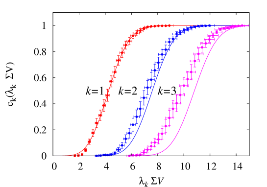
Another non-trivial comparison can be made through the shape of the eigenvalue distributions. We plot the cumulative distribution
| (18) |
of the three lowest eigenvalues in Figure 8. The agreement between the lattice data and ChRMT (solid curves) is quite good for the lowest eigenvalue, while for the higher modes the agreement is marginal. This observation can be made more quantitative by analyzing the moments defined in (9). In Table 3 we list the numerical results of both ChRMT and lattice data for the subtracted moments . The overall agreement is remarkable, though we see deviations of about 10% in the averages. The deviations in the higher moments are larger in magnitude but statistically less significant (less than two standard deviations).
The leading systematic error in the determination of is the finite size effect, which scales as . Unfortunately we can not calculate such a higher order effect within the framework of ChRMT, but we can estimate the size of the possible correction using the higher order calculations of related quantities in ChPT. To the one-loop order, the chiral condensate is written as
| (19) |
where is a numerical constant depending on the lattice geometry Hasenfratz:1989pk . The value for the case of the lattice is 0.0836. Numerically, the correction is 13% assuming the pion decay constant to be = 93 MeV.
The most direct way of reducing the systematic error is to increase the volume, which is very costly, though. Other possibility is to check the results with quantities for which the higher order corrections are known. Meson two-point functions in the -regime are examples of such quantities. A work is in progress to calculate the two-point functions on our gauge ensembles.
We quote the result of in the continuum regularization scheme, i.e. the scheme. We have calculated the renormalization factor using the non-perturbative renormalization technique through the RI/MOM scheme Martinelli:1994ty . Calculation is done on the -regime () lattice with several different valence quark masses. The result is . Details of this calculation will be presented in a separate paper. Including the renormalization factor, our result is
| (20) |
The errors represent a combined statistical error (from , , and ) and the systematic error estimated from the higher order effects in the -expansion as discussed above. Since the calculation is done at a single lattice spacing, the discretization error cannot be quantified reliably, but we do not expect much larger error because our lattice action is free from discretization effects.
V Low-mode spectrum in the -regime
For heavier sea quarks, the -expansion is not justified and the conventional -expansion should be applied instead. Therefore, the correspondence between the Dirac eigenvalue spectrum and ChRMT is not obvious. On the other hand, for heavy enough sea quarks the low-lying eigenvalues should behave as if they are in the quenched lattices. Here we assume that the correspondence is valid in the intermediate sea quark mass region too, and compare the lattice data with the ChRMT predictions for larger . Strictly speaking, the theoretical connection to ChRMT is established only at the leading order of the expansion, which is valid when is satisfied.


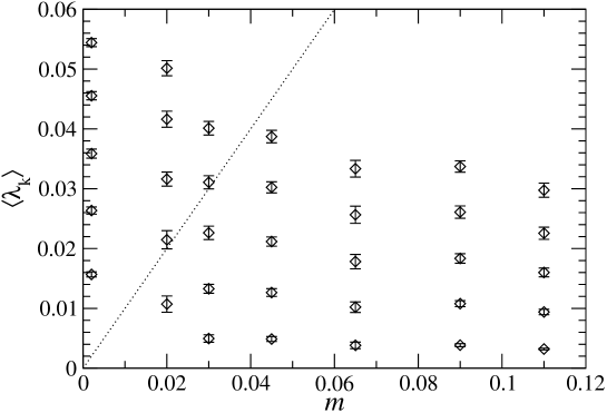
In Figure 9 we plot the eigenvalue ratios ( = 2–4) as a function of . The data are shown for both = 2.35 and 2.30. The curves in the plots show the predictions of ChRMT. The expected transition from the dynamical to quenched lattices can be seen in the lattice data below 10. The mass dependence at = 2.35 is consistent with ChRMT within relatively large statistical errors, while the precise data at = 2.30 show some disagreement especially for third and fourth eigenvalues.
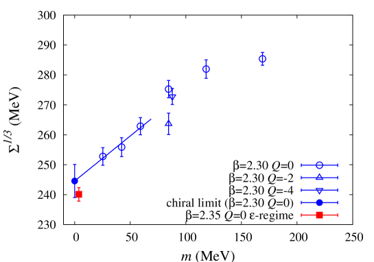
We extract the chiral condensate for each sea quark mass using the same method applied in the -regime taking account of the mass dependence of . The results at = 2.30 are plotted in Figure 10 (open circles). We use a physical unit for both and ; the lattice scale is determined through after extrapolating the chiral limit. The results show a significant sea quark mass dependence. If we extrapolate linearly in sea quark mass using three lowest data points we obtain = [245(5)(6) MeV]3 in the chiral limit. This value is consistent with the result in the -regime as shown in the plot.
In Figure 10 we also plot data points for non-zero topological charge ( and 4) at . We find some discrepancy between and 2 while is consistent with . The size of the disagreement is about 4% for and thus 12% for , which is consistent with our estimate of the higher order effect in the expansion.
VI Bulk spectrum
Although our data for the Dirac eigenvalue spectrum show a qualitative agreement with the ChRMT predictions, there are deviations, which is significant for the larger eigenvalues as seen in Table. 3. This can be understood by looking at higher eigenvalue histogram, which we call the bulk spectrum. Figure 11 shows a histogram of 50 lowest eigenvalues in the -regime ( = 2.35, = 0.002). The normalization is fixed such that it corresponds to the spectral density
| (21) |
divided by the volume in the limit of vanishing bin size.

In order to understand the shape of the data in Figure 11 at least qualitatively, we consider a simple model. Away from the low-mode region one expects a growth of the spectral function as , which is obtained from the number of plain-wave modes of quarks in the free case. By adding the condensate contribution from the Banks-Casher relation Banks:1979yr we plot a dashed curve in Figure 11. Near the microscopic limit , the ChRMT prediction is expected to match with the data, where is defined by (7). We plot the massless case in Figure 11 for a comparison. (Deviation of the spectrum at from the massless case is only %.).
The ChRMT curve gives a detailed description of the Banks-Casher relation: it approaches a constant in the large volume limit. On the other hand, since ChRMT is valid only at the leading order of the expansion, the region of growth cannot be described. Therefore, for the analysis of the microscopic eigenvalues to be reliable, one has to work in a flat region where the contribution is negligible. This is the reason that the lowest eigenvalue is most reliable to extract in our analysis in the previous sections.
From Figure 11 we observe that the flat region does not extend over , which roughly corresponds to the fourth lowest eigenvalue in our data. Already at around this upper limit, the eigenvalues are pushed from above by a repulsive force from the bulk eigenmodes rapidly increasing as , and the ratio is systematically underestimated for = 3 and 4 as found in Figure 7. This effect is regarded as one of the finite size effect, because the term scales as and its magnitude in the microscopic regime is suppressed for larger volumes as . In addition, the peaks of the first few eigenvalues move towards for larger volumes, and thus become less sensitive to the effects from bulk eigenmodes.
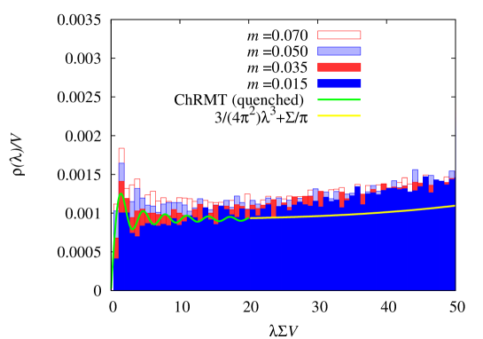
The bulk spectrum for heavier sea quark masses, which are out of the -regime, is also interesting in order to see what happens after the transition to the “quenched-like” region of the eigenvalue spectrum. In Figure 12 the eigenvalue histogram is shown for = 2.30 lattices at = 0.015, 0.035, 0.050 and 0.070, all of which are in the -regime. The plot is normalized with = 0.00212, which is the value after the chiral extrapolation shown in Figure 10. First of all, the physical volume at = 2.30 is about 30% larger than that at = 2.35. Therefore, as explained above, the growth of is expected to be much milder and the lattice data is consistent with this picture. The flat region extends up to around . Second, because the microscopic eigenvalue distribution approaches that of the quenched theory, the lowest peak is shifted towards the left. Overall, the number of eigenvalues in the microscopic region increases a lot. Unfortunately, the correspondence between ChPT and ChRMT is theoretically less clear, since the sea quark masses are in the -regime. In order to describe this region, the standard ChPT must be extended to the partially quenched ChPT and a mixed expansion has to be considered. Namely, the sea quarks are treated in the -expansion, while the valence quarks are put in the -regime to allow the link to ChRMT. In this paper we simply assume that ChRMT can be applied for finite sea quark masses out of the -regime. We observe in Figure 12 that the distribution near the lowest eigenvalue is well described by ChRMT, but the peak grows as the quark mass increases. This means that the effective value of grows as the quark mass increases, which is consistent with the sea quark mass dependence of plotted in Figure 10.
VII Conclusions
We studied the eigenvalue spectrum of the overlap-Dirac operator on the lattices with two-flavors of dynamical quarks. We performed dynamical fermion simulation in the -regime by pushing the sea quark mass down to 3 MeV. For comparison, we also calculated the eigenvalue spectrum on the -regime lattices at two lattice spacings with sea quark mass in the range –. All the runs are confined in a fixed topological charge , except for a few cases with finite .
We found a good agreement of the distribution of low-lying eigenvalues in the -regime with the predictions of ChRMT, which implies a strong evidence of the spontaneous breaking of chiral symmetry in QCD. We extracted the chiral condensate as = [251(7)(11) MeV]3 from the lowest eigenvalue. The renormalization factor was calculated non-perturbatively. The value of contains a systematic error of 10% due to the higher order effect in the expansion . Better determination of will require larger physical volumes to suppress such finite size effects.
Out of the -regime (the case with heavier sea quark masses) the Dirac eigenvalue distribution still shows a reasonable agreement with ChRMT. The value of extracted in this region shows a significant quark mass dependence, while its chiral limit is consistent with the -regime result.
Further information on the low-energy constants can be extracted in the -regime by calculating two- and three-point functions or analyzing the Dirac eigenvalue spectrum with imaginary chemical potential Damgaard:2001js ; Hernandez:2006kz ; Akemann:2006ru . The present work is a first step towards such programs.
ACKNOWLEDGMENTS
We thank P.H. Damgaard and S.M. Nishigaki for useful suggestions and comments. The authors acknowledge YITP workshop YITP-W-05-25 on “Actions and Symmetries in Lattice Gauge Theory” for providing the opportunity to have fruitful discussions. Numerical simulations are performed on IBM System Blue Gene Solution at High Energy Accelerator Research Organization (KEK) under a support of its Large Scale Simulation Program (No. 07-16). This work is supported in part by the Grant-in-Aid of the Japanese Ministry of Education (No. 13135204, 15540251, 16740156, 17740171, 18340075, 18034011, 18740167, and 18840045) and the National Science Council of Taiwan (No. NSC95-2112-M002-005).
References
- (1) J. Gasser and H. Leutwyler, Phys. Lett. B 188, 477 (1987).
- (2) F. C. Hansen, Nucl. Phys. B 345, 685 (1990).
- (3) F. C. Hansen and H. Leutwyler, Nucl. Phys. B 350, 201 (1991).
- (4) H. Leutwyler and A. Smilga, Phys. Rev. D 46, 5607 (1992).
- (5) E. V. Shuryak and J. J. M. Verbaarschot, Nucl. Phys. A 560, 306 (1993) [arXiv:hep-th/9212088].
- (6) A. V. Smilga, arXiv:hep-th/9503049.
- (7) J. J. M. Verbaarschot and T. Wettig, Ann. Rev. Nucl. Part. Sci. 50, 343 (2000) [arXiv:hep-ph/0003017].
- (8) P. H. Damgaard and S. M. Nishigaki, Phys. Rev. D 63, 045012 (2001) [arXiv:hep-th/0006111].
- (9) G. Akemann, P. H. Damgaard, J. C. Osborn and K. Splittorff, Nucl. Phys. B 766, 34 (2007) [arXiv:hep-th/0609059].
- (10) R. G. Edwards, U. M. Heller, J. E. Kiskis and R. Narayanan, Phys. Rev. Lett. 82, 4188 (1999) [arXiv:hep-th/9902117].
- (11) W. Bietenholz, K. Jansen and S. Shcheredin, JHEP 0307, 033 (2003) [arXiv:hep-lat/0306022].
- (12) L. Giusti, M. Luscher, P. Weisz and H. Wittig, JHEP 0311, 023 (2003) [arXiv:hep-lat/0309189].
- (13) J. Wennekers and H. Wittig, JHEP 0509, 059 (2005) [arXiv:hep-lat/0507026].
- (14) K. Ogawa and S. Hashimoto, Prog. Theor. Phys. 114, 609 (2005) [arXiv:hep-lat/0505017].
- (15) T. DeGrand, Z. Liu and S. Schaefer, Phys. Rev. D 74, 094504 (2006) [Erratum-ibid. D 74, 099904 (2006)] [arXiv:hep-lat/0608019].
- (16) C. B. Lang, P. Majumdar and W. Ortner, arXiv:hep-lat/0611010.
- (17) H. Neuberger, Phys. Lett. B 417, 141 (1998) [arXiv:hep-lat/9707022].
- (18) H. Neuberger, Phys. Lett. B 427, 353 (1998) [arXiv:hep-lat/9801031].
- (19) M. Luscher, Phys. Lett. B 428, 342 (1998) [arXiv:hep-lat/9802011].
- (20) H. Fukaya, S. Hashimoto, K. I. Ishikawa, T. Kaneko, H. Matsufuru, T. Onogi and N. Yamada [JLQCD Collaboration], Phys. Rev. D 74, 094505 (2006) [arXiv:hep-lat/0607020].
- (21) H. Fukaya et al. [JLQCD Collaboration], Phys. Rev. Lett. 98, 172001 (2007) [arXiv:hep-lat/0702003].
- (22) G. Martinelli, C. Pittori, C. T. Sachrajda, M. Testa and A. Vladikas, Nucl. Phys. B 445, 81 (1995) [arXiv:hep-lat/9411010].
- (23) P. H. Ginsparg and K. G. Wilson, Phys. Rev. D 25, 2649 (1982).
- (24) P. Hernandez, K. Jansen and M. Lüscher, Nucl. Phys. B 552, 363 (1999) [arXiv:hep-lat/9808010].
- (25) R. G. Edwards, U. M. Heller and R. Narayanan, Nucl. Phys. B 535, 403 (1998) [arXiv:hep-lat/9802016].
- (26) F. Berruto, R. Narayanan and H. Neuberger, Phys. Lett. B 489, 243 (2000) [arXiv:hep-lat/0006030].
- (27) T. Izubuchi and C. Dawson [RBC Collaboration], Nucl. Phys. Proc. Suppl. 106, 748 (2002).
- (28) P. M. Vranas, Phys. Rev. D 74, 034512 (2006) [arXiv:hep-lat/0606014].
- (29) J. van den Eshof, A. Frommer, T. Lippert, K. Schilling and H. A. van der Vorst, Comput. Phys. Commun. 146, 203 (2002) [arXiv:hep-lat/0202025].
- (30) T. W. Chiu, T. H. Hsieh, C. H. Huang and T. R. Huang, Phys. Rev. D 66, 114502 (2002) [arXiv:hep-lat/0206007].
- (31) Y. Iwasaki, Nucl. Phys. B 258, 141 (1985).
- (32) Y. Iwasaki and T. Yoshie, Phys. Lett. B 143, 449 (1984).
- (33) T. Kaneko et al. [JLQCD Collaboration], in preparation.
- (34) R. Sommer, Nucl. Phys. B 411, 839 (1994) [arXiv:hep-lat/9310022].
- (35) Z. Fodor, S. D. Katz and K. K. Szabo, JHEP 0408, 003 (2004) [arXiv:hep-lat/0311010].
- (36) T. A. DeGrand and S. Schaefer, Phys. Rev. D 71, 034507 (2005) [arXiv:hep-lat/0412005].
- (37) N. Cundy, S. Krieg, G. Arnold, A. Frommer, T. Lippert and K. Schilling, arXiv:hep-lat/0502007.
- (38) M. Hasenbusch, Phys. Lett. B 519, 177 (2001) [arXiv:hep-lat/0107019].
- (39) J. C. Sexton and D. H. Weingarten, Nucl. Phys. B 380, 665 (1992).
- (40) N. Cundy, J. van den Eshof, A. Frommer, S. Krieg, T. Lippert and K. Schafer, Comput. Phys. Commun. 165, 221 (2005) [arXiv:hep-lat/0405003].
- (41) H. Matsufuru et al. [JLQCD Collaboration], PoS LAT2006, 031 (2006) [arXiv:hep-lat/0610026].
- (42) H. Neff, N. Eicker, T. Lippert, J. W. Negele and K. Schilling, Phys. Rev. D 64, 114509 (2001) [arXiv:hep-lat/0106016].
- (43) L. Del Debbio, L. Giusti, M. Luscher, R. Petronzio and N. Tantalo, JHEP 0602, 011 (2006) [arXiv:hep-lat/0512021].
- (44) P. Hasenfratz and H. Leutwyler, Nucl. Phys. B 343, 241 (1990).
- (45) T. Banks and A. Casher, Nucl. Phys. B 169, 103 (1980).
- (46) P. H. Damgaard, M. C. Diamantini, P. Hernandez and K. Jansen, Nucl. Phys. B 629, 445 (2002) [arXiv:hep-lat/0112016].
- (47) P. Hernandez and M. Laine, JHEP 0610, 069 (2006) [arXiv:hep-lat/0607027].