Axial $N\to\Delta(1232)$ and $N\to N^{\star}(1440)$ transition form factors

Abstract

We calculate the axial $N\to\Delta(1232)$ and $N\to N^{\star}(1440)$ transition form factors in a chiral constituent quark model. As required by the partial conservation of axial current ($PCAC$) condition, we include one- and two-body axial exchange currents. For the axial $N\to\Delta(1232)$ form factors we compare with previous quark model calculations that use only one-body axial currents, and with experimental analyses. The paper provides the first calculation of all weak axial $N\to N^{\star}(1440)$ form factors. Our main result is that exchange currents are very important for certain axial transition form factors. In addition to improving our understanding of nucleon structure, the present results are relevant for neutrino-nucleus scattering cross section predictions needed in the analysis of neutrino mixing experiments.

I Introduction

The axial $N\to N^{\star}$ transition form factors play an important role in neutrino induced pion production on the nucleon, e.g. in ${\bar{\nu}_{e}}+p\to\Delta^{0}+e^{+}\to n+\pi^{0}+e^{+}$. The two lowest-lying nucleon resonances, $\Delta(1232)$ and $N^{\star}(1440)$ (Roper resonance) are expected to give the dominant contribution to the neutrino scattering cross section for moderate neutrino energies. Weak $\Delta(1232)$ production has been studied experimentally in a series of neutrino scattering experiments on hydrogen and deuterium targets radecky ; barish ; kitagaki . New data on the $N\to\Delta$ axial vector transition form factor are expected from experiments at Jefferson Laboratory latifa . On the theoretical side, the weak axial $\Delta$ excitation has been attracting attention since the 1960’s and has been studied using different approaches. For an overview see Refs. schreiner ; c5q3 . The first lattice computation of $N\to\Delta$ axial form factors has just appeared lattice .

To our knowledge there is no experimental information on the axial $N\to N^{\star}(1440)$ transition form factors. In Ref. luis98 the authors provided a theoretical estimate of the weak $N^{\star}(1440)$ production cross section in electron induced reactions in the kinematic region of the $\Delta$ resonance but no prediction for the axial $N\to N^{\star}(1440)$ form factors was made. The only theoretical determination of weak form factors for the $N\to N^{\star}(1440)$ transition that we are aware of, was done in Ref. bruno but there only one of them, namely $g_{A}^{\star}$ (see below) was evaluated.

It is important to have quark model predictions for the weak $N\to N^{\star}$ transition form factors for two reasons. First, they contain information on the spatial and spin structure of the nucleon and its excited states that is complementary to that obtained from electromagnetic $N\to N^{\star}$ form factors mec . Second, they are required for neutrino-nucleus scattering cross section predictions which in turn are needed for a precise determination of neutrino mass differences and mixing angles Pas04 . Previous quark model calculations c5q3 ; Abd72 ; c5q1 ; c5q1-2 ; c5q2 ; c5q4 ; c5q5 included only one-body axial currents, i.e. processes where the weak probe couples to just one valence quark at a time (impulse approximation). However, this approximation violates the partial conservation of axial current (PCAC) condition, which requires that the axial current operator be a sum of one-body and two-body exchange terms, and that the latter be connected with the two-body potentials of the quark model Hamiltonian david1 ; david2 . The axial exchange currents provide an effective description of the non-valence quark degrees of freedom in the nucleon as probed by the weak interaction.

Recently, employing a chiral quark model with gluon and pseudoscalar meson exchange potentials and corresponding axial exchange currents, we have evaluated the elastic axial nucleon form factors $g_{A}(q^{2})$ and $g_{P}(q^{2})$ david1 , as well as the axial couplings $g^{8}_{A}(0)$ and $g^{0}_{A}(0)$ related to the spin content of the nucleon david2 . The results obtained were in good agreement with experiment. Furthermore, they allowed a consistent quark model interpretation of the missing nucleon spin as orbital angular momentum carried by the nonvalence quark degrees of freedom in the nucleon. In the present paper we apply this model to the weak excitation of nucleon resonances as shown in Fig. 1 and calculate the axial $N\to\Delta(1232)$ and $N\to N^{\star}(1440)$ form factors. As in our previous work, we go beyond the impulse approximation and include not only pion exchange currents but also two-body axial currents arising from gluon exchange and the confinement interaction as required by PCAC. We will see below that in certain axial form factors, the contribution of various exchange currents can be clearly identified, and thus further details of nucleon structure can be revealed.

The paper is organized as follows. After a short review of the chiral quark model in sect. 2, we calculate in sect. 3 all four Adler form factors $C^{A}_{i}(q^{2}),\ i=3\cdots 6$ of the weak $N\to\Delta(1232)$ transition, and compare with other theoretical calculations and experimental analyses of neutrino-induced pionproduction on the nucleon. Sect. 4 is devoted to the axial $N\to N^{\star}(1440)$ transition, for which we present the first theoretical prediction of all three axial form factors. We summarize our results in sect. 5.

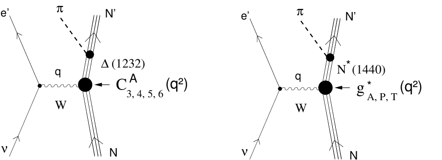
Figure 1: Feynman diagrams for neutrino-induced pionproduction on the nucleon via resonance excitation. Left: Axial transition form factors $C_{3}^{A}(q^{2})$, $C_{4}^{A}(q^{2})$, $C_{5}^{A}(q^{2})$, and $C_{6}^{A}(q^{2})$ contributing to weak $N\to\Delta(1232)$ excitation. Right: Axial transition form factors $g_{A}^{*}(q^{2})$, $g_{P}^{*}(q^{2})$, and $g_{T}^{*}(q^{2})$ contributing to weak excitation of the $N^{*}(1440)$ resonance. The four-momentum transfer of the weak gauge boson $W$ is denoted by $q$.

II Chiral quark model

The calculation of the axial form factors is performed within the framework of the chiral constituent quark model in which chiral symmetry is introduced via the non-linear $\sigma$-model. Although we refer the reader to Ref. david2 for details of the model, we explain here its main ingredients. The Hamiltonian includes apart from a confinement potential $V^{conf}$, a one-gluon exchange potential $V^{g}$, and a one-pion exchange potential $V^{\pi}$ 

$$H=\sum_{j=1}^{3}\left(m_{q}+\frac{\hbox{$p$}\hbox to0.0pt{\hss\hbox{$p$}\hskip 0.39993pt}\hbox to0.0pt{\hss\lower 0.17218pt\hbox{\hbox{$p$}\hbox to0.0pt{\hss\hbox{$p$}\hskip 0.39993pt}}}_{j}^{2}}{2m_{q}}\right)-\frac{\hbox{$P$}\hbox to0.0pt{\hss\hbox{$P$}\hskip 0.39993pt}\hbox to0.0pt{\hss\lower 0.17218pt\hbox{\hbox{$P$}\hbox to0.0pt{\hss\hbox{$P$}\hskip 0.39993pt}}}^{2}}{6m_{q}}+\sum_{j<k=1}^{3}\left(V^{conf}({\bf r}_{j},{\bf r}_{k})+V^{g}({\bf r}_{j},{\bf r}_{k})+V^{\pi}({\bf r}_{j},{\bf r}_{k})\right),$$ (1)

where $m_{q}$ is the constituent quark mass. Here, ${\bf r}_{j}$, ${\bf p}_{j}$ are the position and momentum operators of the $j$-th quark, and ${\bf P}$ is the momentum of the center of mass of the three-quark system. The kinetic energy of the center of mass motion is subtracted from the total Hamiltonian. Explicit expressions for the individual potentials can be found in Ref. david2 .

The axial currents employed in this work are shown in Fig. 2. As mentioned in the introduction, the axial current operator contains not only one-body currents but also two-body gluon, pion, and confinement exchange currents consistent with the two-body potentials in Eq.(1) as required by the PCAC relation

$${\bf q}\cdot{\bf A}({\bf q})-[H,A^{0}({\bf q})]=-i\ \sqrt{2}\ f_{\pi}\frac{m_{\pi}^{2}}{q^{2}-m_{\pi}^{2}}M^{\pi}({\bf q}).$$ (2)

The PCAC equation links the strong interaction Hamiltonian $H$, the weak axial current $A^{\mu}=(A^{0},{\bf A})$ operators, and the pion emission operator described by $M^{\pi}$. Here, $m_{\pi}$ is the pion mass and $f_{\pi}$ is the pion decay constant.

Figure 2: Feynman diagrams for the axial currents employed in this work: a) one-body current (impulse approximation), b) one-gluon exchange current, c) confinement exchange current, d) one-$\pi$ exchange current.

Eq.(2) also demands that the axial coupling of the quarks, $g_{Aq}$, is related to the pion-quark coupling constant, $g_{\pi q}$, via a Goldberger-Treiman relation david1

$$g_{Aq}=f_{\pi}\frac{g_{\pi q}}{m_{q}}.$$ (3)

Inserting the physical values for the constituent quark mass, the pion decay constant, and the pion-quark coupling, one finds that $g_{Aq}$ is renormalized from its bare value of 1 for structureless QCD quarks to 0.77 for constituent quarks.

To solve the Schrödinger equation for the Hamiltonian in Eq.(1) the wave functions are expanded in a harmonic oscillator basis that includes up to $N=2$ excitation quanta. The $N$ ground state and $N^{*}(1440)$ wave functions are given by a superposition of five harmonic oscillator states

$$|N\ \rangle = a_{S_{S}}\ |S_{S}\rangle+a_{S_{S}^{\prime}}\ |S_{S}^{\prime}\rangle+a_{S_{M}}\ |S_{M}\rangle+a_{D_{M}}\ |D_{M}\rangle+a_{P_{A}}\ |P_{A}\rangle$$

$$|N^{\star}\rangle = a^{\star}_{S_{S}}\ |S_{S}\rangle+a^{\star}_{S_{S}^{\prime}}\ |S_{S}^{\prime}\rangle+a^{\star}_{S_{M}}\ |S_{M}\rangle+a^{\star}_{D_{M}}\ |D_{M}\rangle+a^{\star}_{P_{A}}\ |P_{A}\rangle,$$ (4)

while for the $\Delta$ ground state we have

$$|\Delta\rangle=b_{S_{S}}\ |S_{S}\rangle_{\Delta}+b_{S_{S}^{\prime}}\ |S_{S}^{\prime}\rangle_{\Delta}+b_{D_{S}}\ |D_{S}\rangle_{\Delta}+b_{D_{M}}\ |D_{M}\rangle_{\Delta}.$$ (5)

The mixing coefficients for the $N(939)$, $N^{*}(1440)$, and $\Delta(1232)$ wave functions are determined by diagonalization of the Hamiltonian in Eq.(1) in this restricted harmonic oscillator basis, and are given in Table 1 (model $A$). The $N$ and $\Delta$ are mainly in the $S_{S}$ harmonic oscillator ground state, while the $N^{*}(1440)$ is mainly given by the radial excitation state denoted as $S^{\prime}_{S}$. Note that the $D$ state probabilities are typically $1\%$ or less. A complete description of the wave functions in Eqs.(II-5) can be found in Ref. ik2 .

$N$	$a_{S_{S}}$	$a_{S^{\prime}_{S}}$	$a_{S_{M}}$	$a_{D_{M}}$	$a_{P_{A}}$
$A$	0.9585	$-0.1475$	$-0.2344$	$-0.0672$	0.0011
$B$	0.9571	$-0.0723$	$-0.2704$	$-0.0753$	0.0005
$N^{*}$	$a^{\star}_{S_{S}}$	$a^{\star}_{S^{\prime}_{S}}$	$a^{\star}_{S_{M}}$	$a^{\star}_{D_{M}}$	$a^{\star}_{P_{A}}$
$A$	0.1689	0.9832	0.0683	0.0122	$-0.0006$
$B$	0.1211	0.9793	0.1604	0.0232	$-0.0005$
$\Delta$	$b_{S_{S}}$	$b_{S^{\prime}_{S}}$	$b_{D_{S}}$	$b_{D_{M}}$
$A$	0.9564	0.2433	$-0.1303$	0.0957
$B$	0.9283	0.3273	$-0.1406$	0.1069

Table 1: Admixture coefficients for the $N(939)$, $N^{*}(1440)$, and $\Delta(1232)$ states as defined in Eqs.(II-5). Model A: color-screened confinement potential david2 ; model B: quadratic confinement potential with anharmonic terms of Eq.(6).

In order to check the sensitivity of our results with respect to the model of confinement, we employ two confinement potentials. Model $A$ refers to the confinement potential in Ref. david2 , which is linear at short distances and color-screened at large inter-quark distances as a result of quark-antiquark pair creation shen . This is our preferred choice. In model $B$ we use a quadratic (harmonic) dependence on the inter-quark distance $r$ corrected by anharmonic terms

$$V^{conf}({\bf r}_{j},{\bf r}_{k})=-\hbox{$\lambda$}\hbox to0.0pt{\hss\hbox{$\lambda$}\hskip 0.39993pt}\hbox to0.0pt{\hss\lower 0.17218pt\hbox{\hbox{$\lambda$}\hbox to0.0pt{\hss\hbox{$\lambda$}\hskip 0.39993pt}}}^{c}_{j}\cdot\hbox{$\lambda$}\hbox to0.0pt{\hss\hbox{$\lambda$}\hskip 0.39993pt}\hbox to0.0pt{\hss\lower 0.17218pt\hbox{\hbox{$\lambda$}\hbox to0.0pt{\hss\hbox{$\lambda$}\hskip 0.39993pt}}}^{c}_{k}\ \left(a_{c}\,r^{2}+A+\frac{B}{r}+Cr\right).$$ (6)

Here, the color factor $\hbox{$\lambda$}\hbox to0.0pt{\hss\hbox{$\lambda$}\hskip 0.39993pt}\hbox to0.0pt{\hss\lower 0.17218pt\hbox{\hbox{$\lambda$}\hbox to0.0pt{\hss\hbox{$\lambda$}\hskip 0.39993pt}}}^{c}_{j}\cdot\hbox{$\lambda$}\hbox to0.0pt{\hss\hbox{$\lambda$}\hskip 0.39993pt}\hbox to0.0pt{\hss\lower 0.17218pt\hbox{\hbox{$\lambda$}\hbox to0.0pt{\hss\hbox{$\lambda$}\hskip 0.39993pt}}}^{c}_{k}=-8/3$ for quarks in a color-singlet baryon, and $r=|{\bf r}_{j}-{\bf r}_{k}|$ is the relative distance between the two quarks. As in the case of the color screened potential david2 , the confinement parameters together with the quark-gluon coupling $\alpha_{s}$ and the oscillator parameter $b$ of model $B$ have been adjusted using the $N$ and $\Delta$ mass spectrum and low energy nucleon electromagnetic properties (magnetic moments and charge and magnetic radii). The numerical values of these parameters are given in Table 2; the corresponding parameters of model $A$ are listed in Ref. david2 .

$b$	$\alpha_{s}$	$a_{c}$	$A$	$B$	$C$
$[$ fm]		[MeV/fm2]	[MeV]	[MeV fm]	[MeV/fm]
0.5844	1.16	13.141	14.993	$-9.765$	12.152

Table 2: Parameters of the confinement potential in Eq.(6), harmonic oscillator parameter $b$, and gluon-quark coupling $\alpha_{s}$ of model $B$.

III Axial $N\to\Delta$ transition form factors

Following Llewellyn Smith ll one can write the most general form of the axial current for the $N\to\Delta$ transition describing, e.g., neutrino induced pion production on the nucleon as depicted in Fig. 1, as a sum of four axial current terms, each of which is multiplied by a Lorentz-invariant form factor $C_{i}^{A}(q^{2})$ that depends only on the square of four-momentum transfer $q^{2}$

$$\bar{u}_{\Delta\nu}({\bf p^{\prime}})\biggl{[}\frac{C_{3}^{A}(q^{2})}{M_{N}}\left(g^{\mu\nu}q_{\sigma}\gamma^{\sigma}-\gamma^{\mu}q^{\nu}\right)+\frac{C_{4}^{A}(q^{2})}{M^{2}_{N}}\left(g^{\mu\nu}p^{\prime}q-p^{\prime\mu}q^{\nu}\right)$$ (7)

$$\hskip 42.67912pt+C_{5}^{A}(q^{2})g^{\mu\nu}+\frac{C_{6}^{A}(q^{2})}{M^{2}_{N}}q^{\mu}q^{\nu}\biggr{]}\sqrt{3}\,{\bf T}^{\dagger}\ u({\bf p}).$$

Here, ${\bf T}^{\dagger}$ is the 1/2 to 3/2 isospin transition operator with reduced matrix element taken to be one. For the $n\to\Delta^{+}$ or $p\to\Delta^{++}$ transitions one needs the $\bf-T^{\dagger}_{+1}$ component of the isospin transition operator, whereas for $n\to\Delta^{-}$ or $p\to\Delta^{0}$ the $\bf T^{\dagger}_{-1}$ component has to be used . In the following we use the $n\to\Delta^{+}$ transition for global normalization of the axial form factors. In Eq.(7), $u({\bf p})$ and $u_{\Delta\nu}({\bf p}^{\prime})$ are Dirac and Rarita-Schwinger spinors Eri88 respectively for a nucleon with three-momentum ${\bf p}$ and a $\Delta$ with momentum ${\bf p}^{\prime}$. The four-momentum transfer $q$ is given by $q=p^{\prime}-p=(q^{0},{\bf q})$, where $q^{0}$ is the energy transfer, and ${\bf q}$ the three-momentum transfer. All four Adler form factors $C_{i}^{A}(q^{2})$ with $i=3,\cdots 6$ are real from $T$ invariance. Before we evaluate the axial $N\to\Delta$ transition form factors in the chiral quark model, we discuss some of their low-energy properties.

The form factor $C_{5}^{A}(q^{2})$ is the $N\to\Delta$ analogue of the nucleon isovector axial form factor $g_{A}(q^{2})$ . $PCAC$ relates its value at $q^{2}=0$ to the strong $\pi N\Delta$ coupling constant $g_{\pi N\Delta}(0)$ through the non-diagonal Goldberger-Treiman relation

$$C_{5}^{A}(0)=\frac{f_{\pi}}{\sqrt{6}}\frac{g_{\pi N\Delta}(0)}{M_{N}}.$$ (8)

With the empirical value for $g_{\pi N\Delta}$ at the pion mass, as extracted from a $K$-matrix analysis of $\pi N$ scattering phase shifts, $g_{\pi N\Delta}(q^{2}=m^{2}_{\pi})=28.6\pm 0.3$ mukho , and $f_{\pi}=92.4\$ MeV pdg as measured in weak pion decay, $C_{5}^{A}(0)=1.15\pm 0.01$ is obtained.

The form factor $C_{6}^{A}(q^{2})$ is the inelastic analogue of the induced pseudoscalar form factor $g_{P}(q^{2})$ of the nucleon. In the framework of Heavy Baryon Chiral Perturbation Theory (HB$\chi$PT) it has been shown that at low momentum transfers $C_{6}^{A}(q^{2})$ is given as zhu

$$\left.C_{6}^{A}(q^{2})\right|_{HB\chi PT}=\frac{g_{\pi N\Delta}(q^{2})}{\sqrt{6}}f_{\pi}\frac{M_{N}}{m^{2}_{\pi}-q^{2}}-\frac{1}{6\sqrt{6}}\,M_{N}\,f_{\pi}\,g_{\pi N\Delta}(q^{2})\,r_{A}^{2}+{\cal O}(q^{2},m^{2}_{\pi}),$$ (9)

quite analogous to the result obtained for the elastic induced pseudoscalar form factor bernard94 . The first term in Eq.( 9) is the dominant pion-pole form factor, and the second term is the leading order non-pole term, where $r_{A}^{2}$ is the square of the axial $N\to\Delta$ transition radius defined as

$$\left.r_{A}^{2}=\frac{6}{C_{5}^{A}(0)}\frac{d\,C_{5}^{A}(q^{2})}{d\,q^{2}}\right|_{q^{2}=0}.$$ (10)

The weak axial $N\to\Delta$ transition radius $r_{A}^{2}$ as extracted from an analysis of neutrino scattering on deuterium kitagaki , lies in the range (see below)

$$r_{A}^{2}\simeq 0.394\sim 0.477\ {\mathrm{fm}}^{2}.$$ (11)

Combining Eq. (9) and Eq.(11) one gets for the non–pole part of the $C_{6}^{A}$ form factor

$$\left.C_{6}^{A,\ non-pole}(0)\right|_{HB\chi PT}\simeq-\frac{1}{6\sqrt{6}}\,M_{N}\,f_{\pi}\,g_{\pi N\Delta}(0)\,r_{A}^{2}=-(1.71\sim 2.07).$$ (12)

As discussed in Ref. c5q3 the form factor $C_{3}^{A}(q^{2})$ is the axial counterpart of the electric quadrupole ($E2$) transition form factor $G_{E2}(q^{2})$ mec , which is important for determining the shape of the nucleon hen01 . In several analyses (see table 5) $C_{3}^{A}(q^{2})=0$ is assumed. Below, we will see that $C_{3}^{A}(q^{2})$ is mainly determined by pion-exchange currents thereby providing a unique possibility to study the nucleon pion cloud without major interference from valence quark and gluon degrees of freedom. As to $C_{4}^{A}(q^{2})$, in the SU(6) symmetry limit, this form factor is connected with the scalar helicity amplitude c5q3 , which in the electromagnetic case corresponds to the charge quadrupole transition form factor $G_{C2}(q^{2})$ mec . However, unlike the latter $C_{4}^{A}(0)\neq 0$ in the SU(6) symmetry limit. Experimentally, both $C_{3}^{A}(q^{2})$ and $C_{4}^{A}(q^{2})$ are poorly known.

We now proceed and calculate all four axial $N\to\Delta$ transition form factors. To this end we have to convert the Dirac spinors in Eq.(7) into Pauli spinors and extract the corresponding operator structure. Including the normalization factors for the $N$ and $\Delta$ spinors one obtains in the center of mass frame of the resonance

$$A^{0}_{N\Delta}=\sqrt{3}{\bf T}^{\dagger}\left(C_{3}^{A}(q^{2})+C_{4}^{A}(q^{2})\frac{M_{\Delta}}{M_{N}}-C_{6}^{A}(q^{2})\frac{q^{0}}{M_{N}}\right)\sqrt{\frac{E_{N}+M_{N}}{2E_{N}}}\ \frac{\hbox{$\sigma$}\hbox to0.0pt{\hss\hbox{$\sigma$}\hskip 0.39993pt}\hbox to0.0pt{\hss\lower 0.17218pt\hbox{\hbox{$\sigma$}\hbox to0.0pt{\hss\hbox{$\sigma$}\hskip 0.39993pt}}}_{N\Delta}^{[1]}\cdot{\bf q}}{M_{N}}$$

$${\bf A}_{N\Delta}=\sqrt{3}{\bf T}^{\dagger}\Bigg{\{}\hbox{$\sigma$}\hbox to0.0pt{\hss\hbox{$\sigma$}\hskip 0.39993pt}\hbox to0.0pt{\hss\lower 0.17218pt\hbox{\hbox{$\sigma$}\hbox to0.0pt{\hss\hbox{$\sigma$}\hskip 0.39993pt}}}_{N\Delta}^{[1]}\bigg{\{}\left(C_{3}^{A}(q^{2})\frac{M_{\Delta}-M_{N}}{M_{N}}+C_{4}^{A}(q^{2})\frac{M_{\Delta}q^{0}}{M_{N}^{2}}+C_{5}^{A}(q^{2})\right)$$

$$\hskip 109.54327pt-\frac{{\bf q}^{2}}{3M_{N}^{2}}\left({C_{6}^{A}(q^{2})}+{C_{3}^{A}(q^{2})}\frac{2M_{N}}{E_{N}+M_{N}}\right)\bigg{\}}$$

$$\hskip 76.82234pt+\left[\hbox{$\sigma$}\hbox to0.0pt{\hss\hbox{$\sigma$}\hskip 0.39993pt}\hbox to0.0pt{\hss\lower 0.17218pt\hbox{\hbox{$\sigma$}\hbox to0.0pt{\hss\hbox{$\sigma$}\hskip 0.39993pt}}}_{N\Delta}^{[1]}\otimes{Y}^{[2]}(\hat{{\bf q}})\right]^{[1]}\frac{{\bf q}^{2}}{M_{N}^{2}}\frac{\sqrt{8\pi}}{3}\left(C_{6}^{A}(q^{2})+\frac{C_{3}^{A}(q^{2})}{4}\frac{2M_{N}}{E_{N}+M_{N}}\right)$$

$$\hskip 76.82234pt-\left[\hbox{$\sigma$}\hbox to0.0pt{\hss\hbox{$\sigma$}\hskip 0.39993pt}\hbox to0.0pt{\hss\lower 0.17218pt\hbox{\hbox{$\sigma$}\hbox to0.0pt{\hss\hbox{$\sigma$}\hskip 0.39993pt}}}_{N\Delta}^{[2]}\otimes{Y}^{[2]}(\hat{{\bf q}})\right]^{[1]}\frac{{\bf q}^{2}}{M_{N}^{2}}\frac{\sqrt{5\pi}}{\sqrt{6}}C_{3}^{A}(q^{2})\frac{2M_{N}}{E_{N}+M_{N}}\Bigg{\}}\sqrt{\frac{E_{N}+M_{N}}{2E_{N}}}.$$ (13)

The $\hbox{$\sigma$}\hbox to0.0pt{\hss\hbox{$\sigma$}\hskip 0.39993pt}\hbox to0.0pt{\hss\lower 0.17218pt\hbox{\hbox{$\sigma$}\hbox to0.0pt{\hss\hbox{$\sigma$}\hskip 0.39993pt}}}_{N\Delta}^{[j]}$ are tensor operators of rank $j$ defined at the baryon level. They are normalized such that their reduced matrix elements are all equal to one. Furthermore, the energy and three-momentum imparted by the weak probe is denoted respectively by $q^{0}$ and ${\bf q}$, $E_{N}=\sqrt{{\bf q}^{2}+M_{N}^{2}}$, and $Y^{[2]}(\hat{\bf q})$ is a spherical harmonic of rank 2 with ${\hat{\bf q}}={\bf q}/|{\bf q}|$. With the axial current operators of the chiral quark model david2 we can calculate all Adler form factors by comparing our quark model matrix elements with the matrix elements of the baryon level operators in Eq. (13). Numerical results are discussed in the next section.

III.1 $N\to\Delta$ axial form factors at $q^{2}=0$

Our numerical results for the four axial $N\to\Delta$ transition form factors at $q^{2}=0$, obtained with our preferred choice for confinement (model A), are shown in Table 3. In contrast to most model predictions (see Table 5), the axial coupling $C_{3}^{A}(0)$ is non-zero in the present approach. As can be seen from Table 3, the finite value for $C_{3}^{A}(0)$ is mainly due to pion exchange currents. Thus, this observable may be useful for determining the relative importance of gluon and pion degrees of freedom in the nucleon. There are non-zero contributions to $C_{3}^{A}(0)$ already in impulse approximation. However, these are small compared to the $\pi$-exchange current contribution if realistic D state probabilities $P_{D}<1\%$ consistent with the Hamiltonian (see Table 1) are employed.

	Imp	Gluon	Pion	Conf	Total
$C_{3}^{A}(0)$	$-$0.0068	$-$0.0054	0.049	$-$0.0010	0.035
$C_{4}^{A}(0)$	$-0.56$	0.31	0.14	$-0.15$	$-0.26$
$C_{5}^{A}(0)$	0.93	$-0.17$	0.14	0.029	0.93
$C_{6}^{A,\,non-pole}(0)$	0.033	0.28	$-0.30$	$-0.73$	$-0.72$

Table 3: Axial couplings $C_{i}^{A}(0)$ for the $N\to\Delta(1232)$ transition obtained with model A for confinement (color screened confinement). The axial current contributions are denoted as: one-body (imp), gluon exchange current (gluon), pion exchange current (pion), confinement current (conf), total result (total).

For the induced pseudoscalar form factor $C_{6}^{A}(0)$, we evaluate only the non-pole contribution $C_{6}^{A,non-pole}(0)$, i.e. the second term in Eq.(9), which is very small in impulse approximation. Moreover, gluon and pion exchange current contributions cancel to a large extent, so that the scalar confinement current is the dominant contribution. This is also the case for the elastic $g_{P}^{non-pole}(0)$ axial coupling david1 . Our result in Table 3 agrees in sign with the one predicted by Eq.(9) but it is a factor $2\sim 3$ smaller in magnitude. As mentioned above, $C_{6}^{A}(0)$ is dominated by the pion-pole contribution of Eq.(9). The large value $C_{6}^{A,\,pion-pole}(0)\approx 52$ makes the extraction of the small non-pole part a difficult task.

For $C_{4}^{A}(0)$ both one-body and two-body exchange current contributions are similar in size, and exchange currents modify the result obtained in impulse approximation considerably. Because of a cancellation of pion and confinement exchange currents at $q^{2}=0$, the gluon exchange current contribution provides the largest correction to the impulse approximation.

The axial vector coupling $C_{5}^{A}(0)$, which is the counterpart of the axial nucleon coupling $g_{A}(0)$, is completely dominated by the one-body axial current (see Table 3). As in the case of $g_{A}(0)$ david1 , we observe an almost complete cancellation between the different exchange current contributions. Because $C_{5}^{A}(0)$ is numerically the most important axial $N\to\Delta$ coupling, we discuss it in more detail below.

	$C_{5}^{A}(0)$
Quark models	0.97 c5q1 ; c5q1-2	0.83 c5q2	1.17 c5q3	1.06 c5q4	0.87 c5q5	1.5 golli03
Empirical approaches	$1.15\pm 0.23$ barish	$1.39\pm 0.14$ c5q5	$1.1\pm 0.2$ c5e2	$1.22\pm 0.06$ luis
Current algebra	0.98 slaughter

Table 4: Axial coupling $C_{5}^{A}(0)$ for the $N\to\Delta$ transition obtained by different groups. Most of this Table has been adapted from Ref. luis .

In Table 4 we give values for $C_{5}^{A}(0)$ obtained by different groups using quark models c5q5 ; c5q1 ; c5q1-2 ; c5q2 ; c5q3 ; c5q4 ; golli03 or empirical approaches barish ; c5q5 ; c5e2 ; luis that fit the $\nu p\to\Delta^{++}\mu^{-}$ and $\nu d\to n\Delta^{++}\mu^{-}$ cross sections. The empirical approaches employ PCAC and the experimental $\pi N\Delta$ coupling constant $g_{\pi N\Delta}(q^{2}=m^{2}_{\pi})$. We also quote a result obtained using a broken symmetry current algebra approach to QCD slaughter , which does not rely on $PCAC$. The quark model results for $C_{5}^{A}(0)$ are generally smaller than the value obtained from Eq.(8) using PCAC. An exception is the recent calculation by Golli et al. golli03 . Using a linear $\sigma$-model they get $C_{5}^{A}(0)=1.5$, some 25% larger than the $PCAC$ estimate in Eq.(8). According to the authors this comes from a meson contribution that is too large, because in their model only mesons bind the quarks so that their strength is overestimated.

In our model $C_{5}^{A}(0)$ is smaller than expected from Eq.(8) because the axial coupling of the constituent quarks, $g_{Aq}$, is renormalized from its bare value of $1$ to $0.77$. While this renormalization led to the correct axial couplings of the nucleon david1 ; david2 , it is seen here to be responsible for a smaller $C_{5}^{A}(0)$ than expected from $PCAC$ and the empirical $g_{\pi N\Delta}(0)$. Conversely, from our value for $C_{5}^{A}(0)$ in Table 3 and Eq.(8) we would obtain $g_{\pi N\Delta}(0)=22.2$ which is only about 4/5 of the empirical strong $\pi N\Delta$ coupling constant. This is a large discrepancy if we think of the width of the $\Delta(1232)$ resonance. Our value would imply a width $\Gamma_{\Delta}\approx 70$ MeV which is only 60% of the experimental width $\Gamma_{\Delta}\approx 120$ MeV. The ratio $g_{\pi N\Delta}(0)/g_{\pi NN}(0)$ evaluated in the present model (using PCAC to extract $g_{\pi N\Delta}(0)$ from $C_{5}^{A}(0)$) is close to the impulse approximation result $\sqrt{72/25}\approx 1.7$, which is smaller than the empirical ratio $g_{\pi N\Delta}(0)/g_{\pi NN}(0)=2.1$.

The present model is then unable to reproduce, via $PCAC$, the strong coupling constant $g_{\pi N\Delta}$ correctly. On the other hand, it is conceivable that the “experimental” width of the $\Delta$ from which $g_{\pi N\Delta}(0)/g_{\pi NN}(0)=2.1$ is determined contains some non-resonant background contribution and that the true $\pi N\Delta$ coupling constant is actually somewhat smaller Henley . In addition, the above considerations are based on the assumption that the non-diagonal Goldberger Treiman relation in Eq. (8) is satisfied to the same accuracy as the diagonal one. A different explanation of the failure to reproduce the $\Delta$ width is given in the model of Ref. li06-1 where claims are made that a 10% admixture of a $qqqq\bar{q}$ component in the $\Delta$ wave function could enlarge the naive three-quark model width by a factor $2\sim 3$. However, weak form factors have not been evaluated in this model.

	$C_{3}^{A}(0)$	$C_{4}^{A}(0)$	$C_{5}^{A}(0)$	$C_{6}^{A,\,non-pole}(0)$
This work (model A)	0.035	$-0.26$	0.93	$-0.72$
Salin salin	0	$-2.7$	0	0
Adler adler	0	$-0.3$	1.2	0
Bijtebier bijtebier	0	$-2.9\sim-3.6$	1.2	0
Zucker zuck	1.8	$-1.8$	1.9	0
HHM c5q5	0	$-0.29\pm 0.006$	$0.87\pm 0.03$	0
SU(6) c5q3	0	$-0.38$	1.17	0
Isgur-Karl c5q3	$-0.0013$	$-0.66$	1.16	0.032
Isgur-Karl 2 c5q3	0.0008	$-0.657$	1.20	0.042
D-mixing c5q3	0.052	0.052	0.813	$-0.17$
Golli golli03	0	0.141	1.53	1.13

Table 5: Results for the $N\to\Delta$ axial couplings obtained in different models. Most of this Table has been taken from Ref.c5q3 .

In Table 5 we compare our total results for the axial couplings with other model calculations. The ingredients of the baryon level calculations salin ; adler ; bijtebier ; zuck are discussed in detail in Ref. schreiner . The remaining entries in Table 5 refer to quark model calculations. The present model is similar to the Isgur-Karl and Isgur-Karl 2 (IK) quark models c5q3 . The main difference is that in the latter only the one-body axial current is taken into account (impulse approximation) and $g_{Aq}$ is kept to 1, whereas we include axial two-body currents and use the renormalized axial quark coupling $g_{Aq}=0.77$ as required by the PCAC condition.

We have already pointed out that for $C_{5}^{A}(0)$ axial exchange current contributions largely cancel so that the difference between the IK model and the present calculation is mainly due to our use of the renormalized axial quark coupling of Eq.(3). For $C_{4}^{A}(0)$ and $C_{6}^{A,\,non-pole}(0)$ the IK results are similar to our one-body current contribution, whereas for $C_{3}^{A}(0)$, they obtain smaller values than our impulse approximation. The different wave function admixture coefficients and oscillator parameter used here and in Ref. c5q3 are responsible for this discrepancy. In any case, the present results clearly show that the main contribution to $C_{3}^{A}(0)$ and $C_{6}^{A,\,non-pole}(0)$ come from exchange currents. Both axial transition couplings are considerably larger than predicted in impulse approximation. Also $C_{4}^{A}(0)$ is significantly affected by exchange currents. Our total result for $C_{4}^{A}(0)$ is in agreement with the one obtained by Adler (see Table 5) using dispersion relations.

Next, we compare our results with the $D$-mixing model c5q3 , which employs only one-body axial currents and $D$-wave admixture coefficients in the $N$ and $\Delta$ that have been adjusted to reproduce the nucleon axial coupling $g_{A}(0)$ as suggested by Glashow glas , and the electric quadrupole ($E2$) over magnetic dipole ($M1$) ratio in the electromagnetic $N\to\Delta$ transition. The net result is a large $D$-wave probability both in the nucleon ($P_{D}=20\%$) and Delta ($P_{D}=30\%$) wave functions.

As mentioned before, the $C_{3}^{A}$ form factor is the weak axial analogue of the $N\to\Delta$ electric quadrupole ($E2$) transition form factor. The latter is a measure of the deviation of $N$ and $\Delta$ shape from spherical symmetry. In the $D$-state mixing model the finite values obtained for $C_{3}^{A}(0)$ and $C_{6}^{A,\,non-pole}(0)$ are a reflection of the nonspherical $N$ and $\Delta$ shape. However, in this model the sizes and signs of the $D$-state admixtures, and the axial current operator are not compatible with the Hamiltonian of the system, and, as a result, the PCAC condition is severely violated. In a consistent theory which includes both one- and two-body axial currents satisfying the PCAC constraint of Eq.(2), the nonsphericity of the $N$ and $\Delta$ comes mainly from the non-valence quark degrees of freedom described by the two-body axial currents and not from highly deformed valence quark orbits as represented by large $D$-state admixtures.

III.2 $q^{2}$ dependence of the axial $N\to\Delta$ form factors

In this section we discuss the $q^{2}$ behavior of the axial transition form factors. The available experimental information comes from the analysis of neutrino scattering experiments radecky ; barish ; kitagaki . Here, we refer to the analysis done by Kitagaki et al. kitagaki where no attempt was made to obtain independent information on the different form factors. Instead, the authors used the Adler model adler as developed by Schreiner and von Hippel schreiner . There, the axial form factors for the $N\to\Delta$ transition have been parametrized as

$$C_{j}^{A}(q^{2})=\frac{C_{j}^{A}(0)\ (1-a_{j}q^{2}/(b_{j}-q^{2}))}{(1-q^{2}/M_{A}^{2})^{2}}\hskip 28.45274pt;\hskip 28.45274ptj=3,4,5$$ (14)

with

$$C_{3}^{A}(0)=0\hskip 5.69046pt,\hskip 5.69046ptC_{4}^{A}(0)=-0.3\hskip 5.69046pt,\hskip 5.69046ptC_{5}^{A}(0)=1.2$$

$$a_{3}=b_{3}=0\hskip 5.69046pt,\hskip 5.69046pta_{4}=a_{5}=-1.21\hskip 5.69046pt,\hskip 5.69046ptb_{4}=b_{5}=2\ {\mathrm{GeV}^{2}}.$$ (15)

In addition, it has been assumed that $C_{6}^{A}(q^{2})$ is given by the pion pole contribution alone. The axial mass $M_{A}$ is the only free parameter which has been adjusted to experiment with the result

$$M_{A}=1.28\ ^{+0.08}_{-0.10}\ {\mathrm{GeV}}.$$ (16)

In this parameterization, the axial radius as defined in Eq.(10) is given by

$$r_{A}^{2}=6\left(\frac{2}{M_{A}^{2}}-\frac{a_{5}}{b_{5}}\right)$$ (17)

from where one gets the values in Eq.(11).

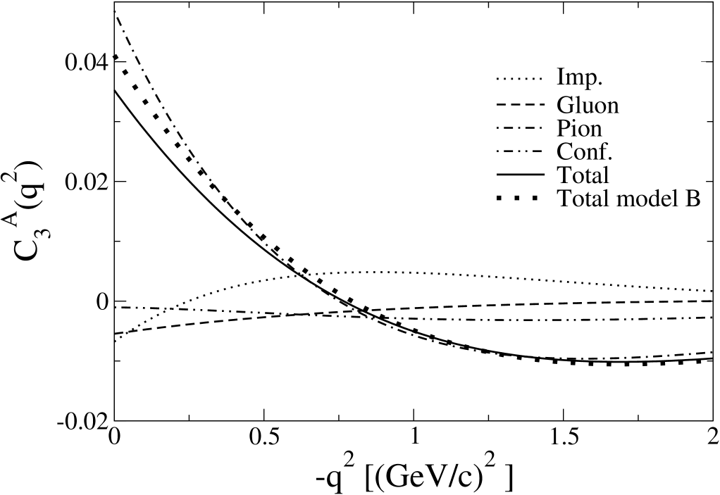
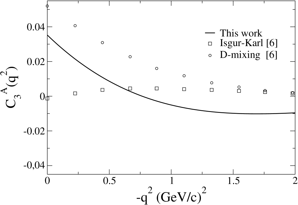
Figure 3: Axial form factor $C_{3}^{A}(q^{2})$. Upper panel: present model calculations with color screened confinement (model A). The individual axial current contributions are denoted as: impulse contribution (dotted line), gluon exchange current (dashed line), pion exchange current (dashed-dotted line), confinement exchange current (dashed-double-dotted line), total result (solid line). The curve labelled Total model $B$ (dotted line, filled squares) represents our total result when using the confinement potential of Eq.(6). Lower panel: comparison with other model calculations. This work (solid line) represents our total result obtained with our preferred choice for confinement (model A), Isgur-Karl model c5q3 (open squares), D-mixing model c5q3 (open circles). There is no experimental information on $C_{3}^{A}(q^{2})$.

In order to compare with experimental data and other theoretical calculations we evaluate the $q^{2}$ dependence of the form factors up to $q^{2}=2$ (GeV/c)² with the caveat that the model may not be reliable at high momentum transfers. For the momentum transfer dependence of the axial constituent quark coupling, $g_{Aq}(q^{2})$, we use axial vector meson dominance

$$g_{Aq}(q^{2})=\frac{g_{Aq}}{1-q^{2}/m^{2}_{a_{1}}}$$ (18)

with $m_{a_{1}}=1260$ MeV, in analogy to the usual vector meson dominance for the electromagnetic quark form factor mec .

In Fig. 3 we show our results for $C_{3}^{A}(q^{2})$. We get non-zero, though small, values which are mainly due to the pion exchange current contribution. The form factor rapidly decreases with $-q^{2}$. In the lower panel of this figure we also show the results obtained in the Isgur-Karl (impulse approximation) model c5q3 leading to very small values over the whole $q^{2}$ range. In the D-mixing model calculation c5q3 , also performed in impulse approximation, but in this case with an unrealistic $D$-state probability in the $N$ and $\Delta$ wave functions, larger values are obtained. Lattice data lattice , not shown in the figure, are compatible with zero within errors, just as assumed in the experimental analysis.

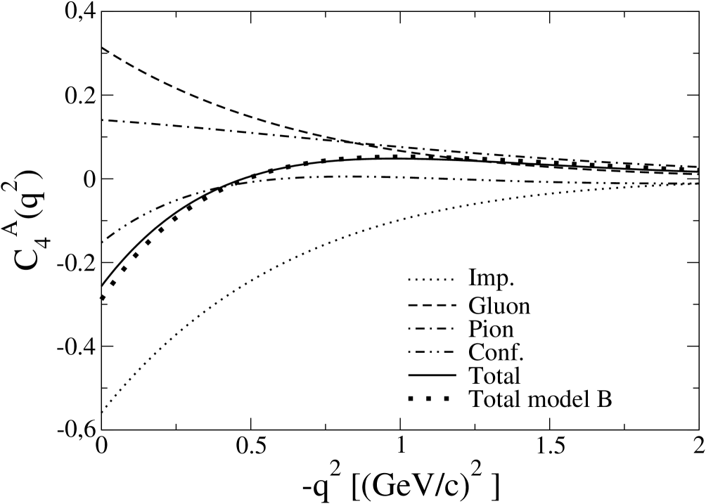
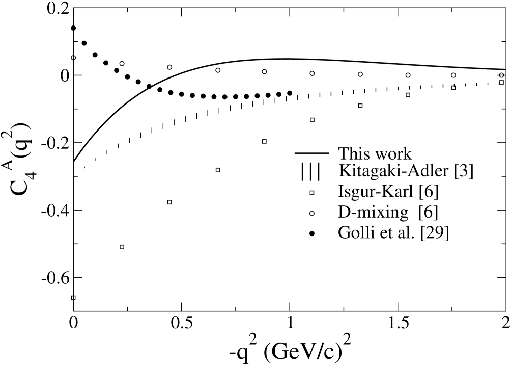
Figure 4: Axial form factor $C_{4}^{A}(q^{2})$. Notation as in figure 3. In the lower panel we also show the results of the Kitagaki-Adler experimental analysis kitagaki (vertical bars), and the ones obtained in the linear $\sigma$-model of Golli et al. golli03 (black circles).

In Fig. 4 we plot the form factor $C_{4}^{A}(q^{2})$. Our total result starts out as expected from the $C_{4}^{A}(q^{2})=-C_{5}^{A}(q^{2})/4$ relation assumed in the experimental analysis, but it soon deviates from it. Exchange currents are responsible for a sign change at around $-q^{2}=0.48$ (GeV/c)². The results of Golli et al. golli03 , obtained in a linear $\sigma$-model calculation, are similar in magnitude to ours but have the opposite sign. They also show a sign change at approximately $-q^{2}=0.24$ (GeV/c)². The Isgur-Karl model calculation c5q3 is very similar to our impulse contribution except for a difference in the normalization at $q^{2}=0$, which, as discussed before, comes from the different $g_{Aq}$ values used in both calculations. In the D-mixing model c5q3 very small and positive values are obtained.

The results from the Kitagaki-Adler experimental analysis kitagaki are also shown in Fig. 4 with vertical bars. The size of the bars reflects the uncertainties in the determination of the axial mass $M_{A}$ (see Eq.(16)). Quenched lattice results lattice display a similar behavior as the one obtained in the calculation of Golli et al. golli03 . On the other hand, unquenched lattice calculations give much larger and positive values in the $0\leq-q^{2}\leq 2$ GeV² region. Apparently, $C_{4}^{A}(q^{2})$ is very sensitive to unquenching and more statistics is needed to draw a firm conclusion concerning its behavior alexandrou06 . In any case, it seems that the assumption $C_{4}^{A}(q^{2})=-C_{5}^{A}(q^{2})/4$ made in the experimental analysis is neither confirmed by quark models nor by lattice determinations.

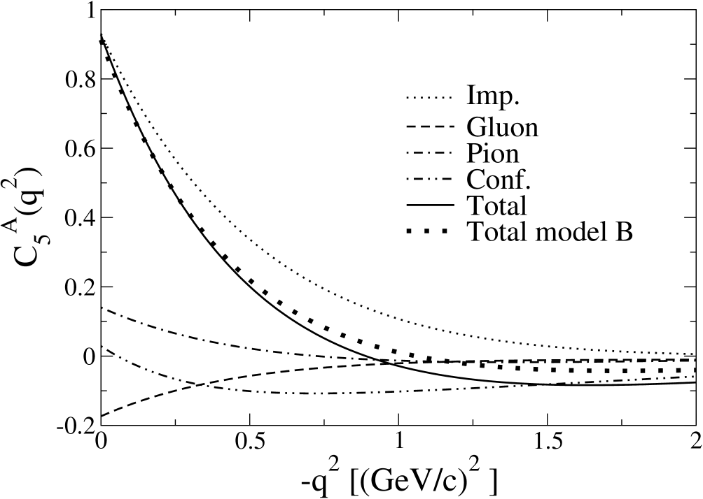
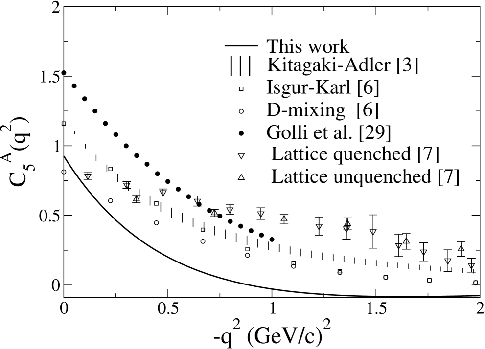
Figure 5: Axial form factor $C_{5}^{A}(q^{2})$. Same notation as in Fig. 4. In the lower panel we also show quenched (down triangles) and unquenched (up triangles) lattice data from Ref. lattice .

In Fig. 5 we present the results for $C_{5}^{A}(q^{2})$. For this observable the impulse contribution is dominant. In the low $q^{2}$ region we predict a similar behavior as the Kitagaki-Adler analysis although with a larger slope at the origin. Our result for the axial radius $\left.r_{A}^{2}\right|_{\mathrm{This\ work}}=0.59\$fm² would be closer to the one obtained in the experimental analysis if we did not include the axial vector meson dominance factor in Eq.(18). The finite axial radius of the constituent quark david1 contributes $r_{Aq}^{2}=0.147$ fm² to the axial transition radius. However, in the low $q^{2}$ region the main difference between the present calculation and the experimental analysis is the normalization $C_{5}^{A}(0)$. We obtain $C_{5}^{A}(0)=0.93$, to be compared to $C_{5}^{A}(0)=1.21$ used in the Kitagaki-Adler analysis. Again our use of the quark axial coupling $g_{Aq}=0.77$ is responsible for this difference.

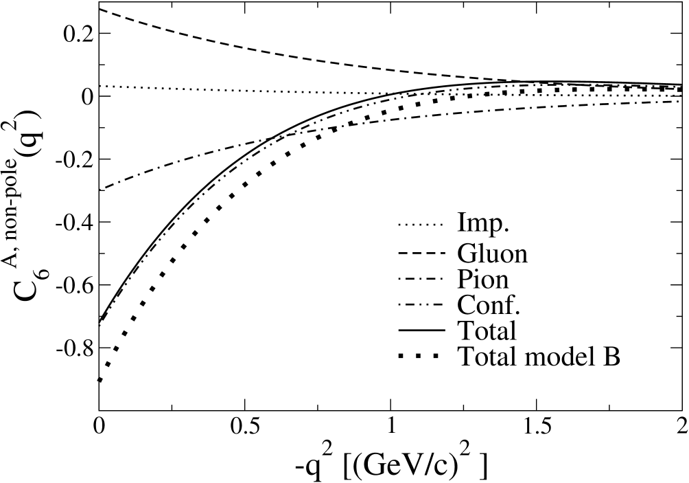
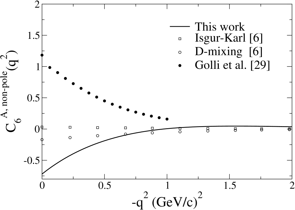
Figure 6: Non-pole part of the axial form factor $C_{6}^{A}(q^{2})$. Notation as in Fig. 4.

The $\sigma$ model calculation of Golli et al. golli03 leads to a similar $q^{2}$ dependence at low momentum transfers as the present calculation but with larger $C_{5}^{A}(q^{2})$ values, in particular they obtain $C_{5}^{A}(0)=1.5$. The Isgur-Karl model c5q3 and our impulse contribution differ mainly in the normalization and good agreement with the experimental analysis is obtained although with a smaller axial radius, $\left.r_{A}^{2}\right|_{\mathrm{Isgur-Karl}}\simeq 0.32\$fm² (our estimate). The axial coupling $C_{5}^{A}(0)$ of the $D$-mixing model c5q3 is similar to our result but the $q^{2}$ dependence of the form factor is different leading to a small axial radius that we estimate to be around $\left.r_{A}^{2}\right|_{\mathrm{D-mixing}}\simeq 0.30\$fm². Quenched lattice data from Ref. lattice hint at a value $\left.C_{5}^{A}(0)\right|_{Latt.\ quenched}\approx 0.86$ (our estimate from a linear extrapolation of their data) with a small axial radius that we estimate as $\left.r_{A}^{2}\right|_{Latt.\ quenched}\approx 0.18$ fm² (our estimate).

Finally, in Fig. 6 we give our results for the form factor $C_{6}^{A,non-pole}(q^{2})$. The one-body contribution is very small, while gluon and pion exchange contributions cancel to a large extent so that the confinement exchange contribution is responsible for the absolute size and shape of this form factor. The results of Golli et al. golli03 are similar in magnitude to the present calculation but, in contrast to our result they predict a positive value. This seems to contradict the findings of HB$\chi$PT zhu where a large negative value for $C_{6}^{A,\ non-pole}(0)$ has been obtained. In the Isgur-Karl model calculation of Ref. c5q3 small and positive values originating from the small $D$-wave components of the $N$ and $\Delta$ wave functions are obtained. On the other hand, the $D$-mixing model calculation of Ref. c5q3 with its large $D$-wave components leads to a negative $C_{6}^{A,non-pole}(q^{2})$, although much smaller in magnitude than the present calculation. There is no lattice calculation of $C_{6}^{A,non-pole}(q^{2})$.

Comparing our results for the color screened confinement potential with the ones for the quadratic plus anharmonic type (Total model $B$ in figs. 3, 4, and 5) we conclude that there a no significant differences for the $C_{3}^{A}(q^{2}),\,C^{A}_{4}(q^{2})$, and $C^{A}_{5}(q^{2})$ form factors. In the case of $C^{A}_{6}(q^{2})$ we observe a $25\%$ change at small $-q^{2}$, with $C^{A}_{6}$ becoming more negative and thus in better agreement with the HB$\chi$PT result zhu .

IV Axial $N\to N^{*}(1440)$ transition form factors

For the $n\to N^{\star+}(1440)$ transition used to normalize the form factors , the axial current can be written as

$$\bar{u}_{\star}({\bf p}^{\prime})\left(g^{\star}_{A}(q^{2})\ \gamma^{\mu}\gamma_{5}+2\frac{M_{N}}{m^{2}_{\pi}}\ g^{\star}_{P}(q^{2})\ q^{\mu}\gamma_{5}+g^{\star}_{T}(q^{2})\ P^{\mu}\gamma_{5}\ \right)u({\bf p}),$$ (19)

where $u({\bf p})$ and $u_{\star}({\bf p}^{\prime})$ are the Dirac spinors for the neutron and the $N^{\star+}(1440)$ with momentum ${\bf p}$ and ${\bf p}^{\prime}$ respectively, and $P=p^{\prime}+p=(P^{0},{\bf P})$. Again the three form factors are real from $T$ invariance. Because the transition is not between members of the same isospin multiplet, invariance of strong interactions under G-parity transformations does not require $g^{\star}_{T}(q^{2})$ to vanish as in the case of the corresponding elastic axial form factor david1 .

Before we present the results of our model calculation, we first discuss some general properties of the $N\to N^{*}(1440)$ transition form factors. As in the diagonal axial $N\to N$ transition, the pseudoscalar form factor $g^{\star}_{P}(q^{2})$ consists of two terms, a pion pole and a non-pole term

$$g^{\star}_{P}(q^{2})=g^{\star\,pion-pole}_{P}(q^{2})+g^{\star\,non-pole}_{P}(q^{2}).$$ (20)

The pseudoscalar form factor $g^{\star}_{P}(q^{2})$ is dominated by the pion-pole contribution given by

$$g^{\star,pion-pole}_{P}(q^{2})=\frac{g_{\pi NN^{\star}}(q^{2})}{2M_{N}}\,f_{\pi}\frac{m^{2}_{\pi}}{M_{N}}\frac{M_{N}+M_{N^{\star}}}{m^{2}_{\pi}-q^{2}},$$ (21)

where $g_{\pi NN^{\star}}(q^{2})$ is the strong $\pi NN^{\star}$ coupling constant assuming a pseudovector $\pi NN^{\star}$ coupling. A determination of this coupling constant from the analysis of the Roper decay into nucleon plus pion assuming a total width of $350\$MeV and a branching ratio of 65% pdg , gives $g_{\pi NN^{\star}}(q^{2}=m^{2}_{\pi})=5.17$. In the case of the $N\to N^{\star}(1440)$ transition, $PCAC$ relates the strong coupling constant $g_{\pi NN^{\star}}(0)$ to the form factors $g^{\star}_{A}(0)$ and $g^{\star}_{T}(0)$ through

$$g^{\star}_{A}(0)+(M_{N^{\star}}-M_{N})\cdot g^{\star}_{T}(0)=f_{\pi}\frac{g_{\pi NN^{\star}}(0)}{M_{N}}.$$ (22)

The operator structure at the baryon level extracted from Eq.(19), including also the normalization factors for the $N$ and $N^{*}(1440)$ spinors, is given in the center of mass of the resonance by

$$A^{0}=\frac{\hbox{$\sigma$}\hbox to0.0pt{\hss\hbox{$\sigma$}\hskip 0.39993pt}\hbox to0.0pt{\hss\lower 0.17218pt\hbox{\hbox{$\sigma$}\hbox to0.0pt{\hss\hbox{$\sigma$}\hskip 0.39993pt}}}\cdot{\bf q}}{E_{N}+M_{N}}\left(-g^{\star}_{A}(q^{2})-q^{0}\frac{2M_{N}}{m^{2}_{\pi}}\,g^{\star}_{P}(q^{2})-P^{0}\ g^{\star}_{T}(q^{2})\right)\sqrt{\frac{E_{N}+M_{N}}{2E_{N}}}$$

$${\bf A}=\hbox{$\sigma$}\hbox to0.0pt{\hss\hbox{$\sigma$}\hskip 0.39993pt}\hbox to0.0pt{\hss\lower 0.17218pt\hbox{\hbox{$\sigma$}\hbox to0.0pt{\hss\hbox{$\sigma$}\hskip 0.39993pt}}}\biggl{[}g^{\star}_{A}(q^{2})-\left(\frac{2M_{N}}{m^{2}_{\pi}}\ g^{\star}_{P}(q^{2})-g^{\star}_{T}(q^{2})\right)\frac{{\bf q}^{2}}{3(E_{N}+M_{N})}\biggr{]}\sqrt{\frac{E_{N}+M_{N}}{2E_{N}}}$$

$$\hskip 22.76228pt+[\hbox{$\sigma$}\hbox to0.0pt{\hss\hbox{$\sigma$}\hskip 0.39993pt}\hbox to0.0pt{\hss\lower 0.17218pt\hbox{\hbox{$\sigma$}\hbox to0.0pt{\hss\hbox{$\sigma$}\hskip 0.39993pt}}}^{[1]}\otimes{\bf q}^{[2]}]^{[1]}\ \sqrt{\frac{5}{3}}\ \frac{1}{E_{N}+M_{N}}\left(\frac{2M_{N}}{m^{2}_{\pi}}\ g^{\star}_{P}(q^{2})-g^{\star}_{T}(q^{2})\right)\sqrt{\frac{E_{N}+M_{N}}{2E_{N}}}.$$ (23)

Here, $\sigma$$\sigma$ $\sigma$$\sigma$  is the Pauli spin matrix operator at the baryon level and ${\bf q}^{[2]}_{m}=[{\bf q}\otimes{\bf q}]^{[2]}_{m}={\bf q}^{2}\sqrt{8\pi/15}\ Y^{[2]}_{m}({\hat{\bf q}})$. These are the appropriate expressions to compare with our explicit constituent quark model calculation in order to extract the axial $N\to N^{\star}(1440)$ transition form factors.

IV.1 $N\to N^{\star}(1440)$ axial form factors at $q^{2}=0$

	Imp	Gluon	Pion	Conf	Total
$g^{\star}_{A}(0)$	$-0.149$	0.169	$-0.169$	$2.5\ 10^{-3}$	$-0.148$
$g^{\star,non-pole}_{P}(0)$	0.0038	$-0.0030$	0.0022	$-0.0097$	$-0.0067$
$g^{\star}_{T}(0)$ [$\mathrm{MeV}^{-1}$]	$3.3\ 10^{-4}$	$-2.8\ 10^{-5}$	$1.7\ 10^{-5}$	$1.7\ 10^{-4}$	$4.9\ 10^{-4}$

Table 6: Axial couplings of the $N\to N^{*}(1440)$ transition obtained with model A for confinement (color screened confinement). The different axial exchange current contributions are denoted as in Table 3.

Our results for the different axial couplings, obtained with our preferred choice for confinement (model A) are given in Table 6. As in the case of $C_{5}^{A}(0)$ discussed above, $g^{\star}_{A}(0)$ is dominated by the one-body axial current. The different two-body currents cancel to a large extent and the total value differs from the impulse result by less than 1% . The weak axial coupling constant $g^{\star,non-pole}_{P}(0)$ is dominated by confinement exchange currents. This is similar to our result for the $N\to\Delta$ form factor $C_{6}^{A,non-pole}(0)$ discussed above. The axial coupling $g^{\star}_{T}(0)$ is non zero, and receives the largest contribution from the one-body axial current.

Using our numerical results of Table 6 for $g^{\star}_{A}(0)$ and $g^{\star}_{T}(0)$, the evaluation of the left-hand side of Eq.(22) yields 

$$g_{\pi NN^{\star}}(0)=1.43,$$ (24)

which is too small compared to the phenomenological value quoted above. Although there is a theoretical analysis krehl of the Roper width that suggests that it could be smaller, i.e., $160\$ MeV rather than $350\$ MeV, the present $g_{\pi NN^{\star}}(0)$ would still be too small. Eq.(24) is also at variance with Ref. riska , where $g_{\pi NN^{\star}}(0)\approx 3.5$ was obtained. On the other hand, their calculation is equivalent to our one-body axial current calculation, and thus both results for $g_{\pi NN^{\star}}(0)$ should agree. In the meantime, the correctness of our finding in Eq.(24) has been been confirmed riskaprivate . A more recent determination by the same group, using a Poincaré covariant constituent quark model with instant, point, and front forms of relativistic kinematics, gives values for $g_{\pi NN^{\star}}$ in the range $g_{\pi NN^{\star}}(0)=0.71\sim 1.11$ depending on the form used bruno in agreement with our determination.

It has been suggested in Ref. jaffe that the $N^{*}(1440)$ resonance could be a pentaquark state that lies in the near-ideally mixed $\overline{10}_{f}\oplus 8_{f}$ representation of SU(3)_f. This suggestion has been further supported by a QCD sum rule calculation matheus . Unfortunately, the expected width is again too small. However, the Roper width is not the only problem posed for the pentaquark interpretation. There is also the problem that recent experimental results have not confirmed previous claims concerning the existence of pentaquark states schumacher . A different analysis argues that the Roper width can be reproduced in a model where the Roper wave function has a 30% admixture of a $qqqq\bar{q}$ component li06-2 . As in the case of the $N\to\Delta$ transition, weak form factors have not yet been evaluated in this model.

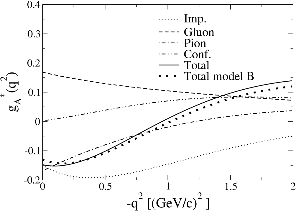
Figure 7: Axial form factor $g_{A}^{\star}(q^{2})$. Notation as in the upper panel of Fig. 3.

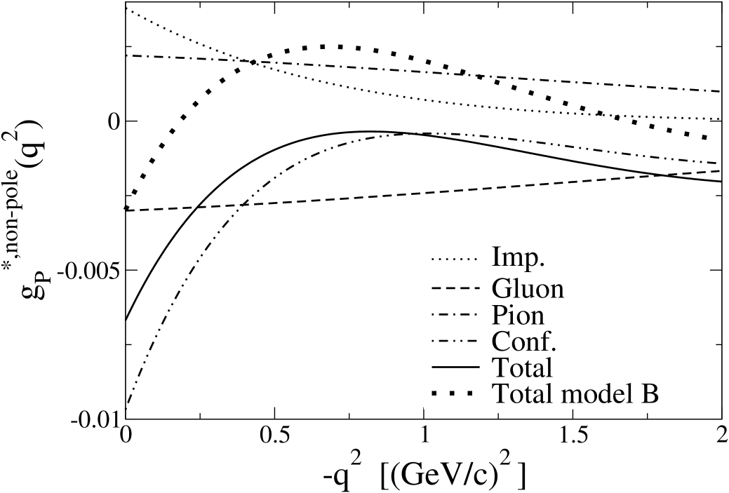
Figure 8: Non-pole part of the axial form factor $g_{P}^{\star}(q^{2})$. Notation as in the upper panel of Fig. 3.

IV.2 $q^{2}$ dependence of the axial $N\to N^{\star}(1440)$ form factors

Next, we discuss the $q^{2}$ behavior of the three $N\to N^{\star}(1440)$ form factors. In Fig. 7 we show $g_{A}^{\star}(q^{2})$. We see that gluon and pion exchange contributions cancel to a large extent over the whole range of momentum transfers considered. At very low $-q^{2}$ the total result is dominated by the one-body axial current, while the confinement exchange current contribution grows as $-q^{2}$ increases. As a result, the minimum in the form factor moves to lower $-q^{2}$ values and we predict a sign change around $q^{2}\approx 1$ GeV². The present impulse approximation is close in shape to the calculation of Ref. bruno using the instant and front form of relativistic kinematics .

Our results for the $g_{P}^{\star,non-pole}(q^{2})$ form factor are shown in Fig. 8. Again, gluon and pion contributions cancel each other to a large extent. The confinement exchange current is the dominant term at low momentum transfers but its contribution decreases in magnitude with increasing $-q^{2}$.

The form factor $g_{T}^{\star}(q^{2})$ displayed in Fig. 9 is non-zero over the entire range of momentum transfers. Gluon and pion contributions are small and the total value at low $q^{2}$ is mainly given by the one-body axial current with confinement exchange current also playing a role. The value for $g_{T}^{\star}(q^{2})$ shows a steady decrease as $-q^{2}$ increases.

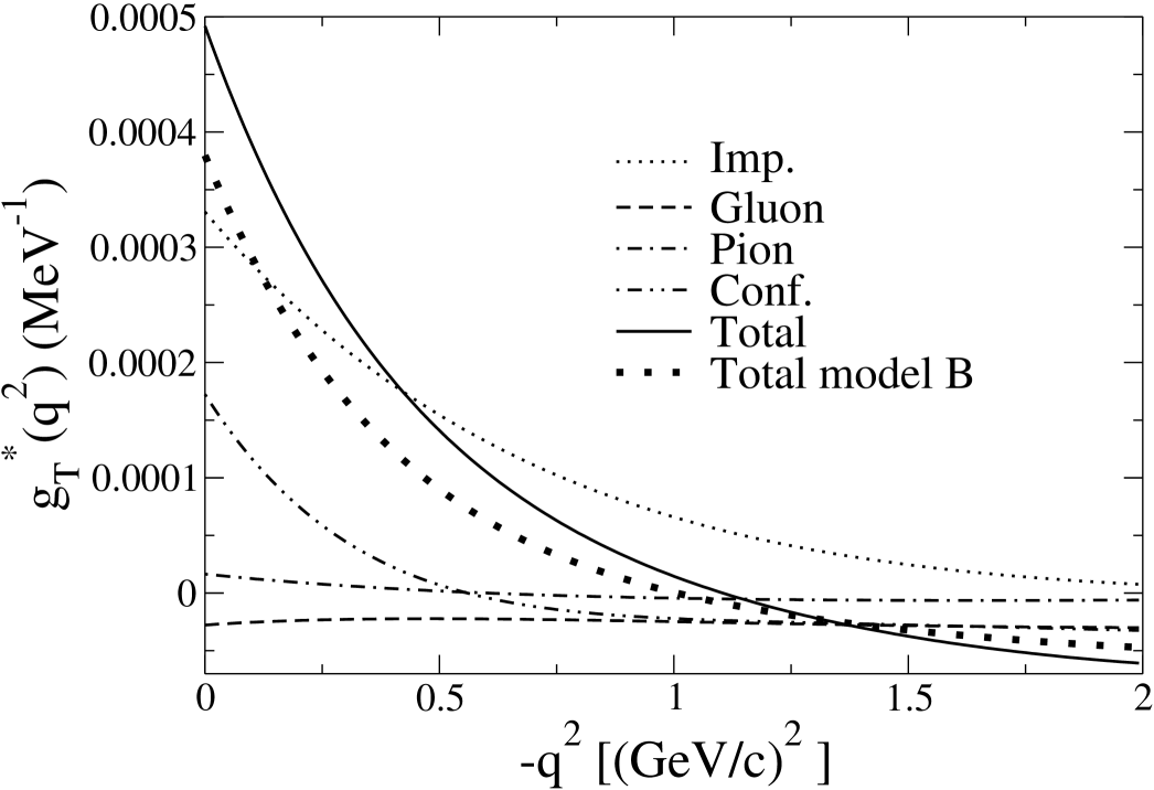
Figure 9: Axial form factor $g_{T}^{\star}(q^{2})$. Notation as in the upper panel of Fig. 3.

Comparison of the results with the ones obtained with the quadratic plus anharmonic confinement potential (Total model $B$ in figs. 7, 8, and 9) shows large changes for $g_{P}^{\star,non-pole}(q^{2})$ due to a decrease (in absolute value) of the confinement contribution. For $g_{A}(q^{2})$ and $g_{T}(q^{2})$ the changes are not that drastic and the general trend of the form factors is preserved.

V Summary

We have investigated the axial form factors of the weak $N\to\Delta(1232)$ and $N\to N^{\star}(1440)$ transitions in a chiral quark model where chiral symmetry is introduced via a non-linear $\sigma$-model. In contrast to previous quark model calculations, we include not only one-body currents but also two-body axial exchange currents consistent with the two-body potentials in the Hamiltonian as required by the PCAC condition.

For the axial $N\to\Delta(1232)$ transition we find that the form factors $C_{3}^{A}(q^{2})$ and $C_{6}^{A,\,non-pole}(q^{2})$ are dominated by two-body currents. In particular, $C_{3}^{A}(q^{2})$ is mainly determined by pion, while $C_{6}^{A,\,non-pole}(q^{2})$ is entirely given by the scalar confinement exchange currents. Also the form factor $C_{4}^{A}(q^{2})$ receives important contributions from axial two-body currents, mainly from the gluon exchange current. On the other hand, due to cancellation of the various exchange current contributions, $C_{5}^{A}(q^{2})$ is governed by the one-body axial current. At $q^{2}=0$ its magnitude is smaller than expected from $PCAC$ and the empirical strong coupling constant, $g_{\pi N\Delta}$, i.e., our result for $C_{5}^{A}(0)$ does not reproduce, via $PCAC$, the experimental value for the strong coupling constant ratio $g_{\pi N\Delta}/g_{\pi NN}$.

For the $N\to N^{\star}(1440)$ transition, we find that $g_{A}^{\star}(q^{2})$ is governed by the one-body axial current but with important corrections coming from scalar confinement exchange currents resulting in a sign change of this form factor at $q^{2}\approx 1$ GeV². At $q^{2}=0$ it agrees with other quark model determinations bruno , but it is too small to explain, via $PCAC$, the empirical value for the strong coupling constant $g_{\pi NN^{\star}}$ obtained from the experimental Roper resonance width. The form factor $g_{P}^{\star,\,non-pole}(q^{2})$ receives the largest contribution from two-body currents, in particular the confinement exchange current. For $g_{T}^{\star}(0)$ we get a non-zero value mainly due to the one-body axial current but with a 30% contribution coming from exchange currents.

In summary, we have found that axial two-body exchange currents play an important role in the weak excitation of nucleon resonances. In particular, the axial $N\to\Delta$ transition form factor $C_{3}^{A}(q^{2})$, which is a measure of the nonsphericity of the $N$ and $\Delta$, is mainly determined by pion exchange currents and thus provides an interesting observable for studying the role of pions in the nucleon without interference from valence quark and gluon degrees of freedom. On the other hand, $C_{6}^{A,\,non-pole}(q^{2})$ is almost exclusively determined by the confinement exchange current. Also the pseudoscalar form factor $g_{P}^{\star,\,non-pole}(q^{2})$ in the $N\to N^{\star}(1440)$ transition is largely governed by the confinement exchange current and sensitive to the confinement model. Further theoretical and experimental investigation of the axial $N\to N^{\star}$ transition form factors will undoubtedly be very useful for obtaining a detailed picture of nucleon structure.