Systematic Errors in the Hubble Constant Measurement
from the Sunyaev-Zel’dovich effect

Abstract

The Hubble constant estimated from the combined analysis of the Sunyaev-Zel’dovich effect and X-ray observations of galaxy clusters is systematically lower than those from other methods by 10-15 percent. We examine the origin of the systematic underestimate using an analytic model of the intracluster medium (ICM), and compare the prediction with idealistic triaxial models and with clusters extracted from cosmological hydrodynamic simulations. We identify three important sources for the systematic errors; density and temperature inhomogeneities in the ICM, departures from isothermality, and asphericity. In particular, the combination of the first two leads to the systematic underestimate of the ICM spectroscopic temperature relative to its emission-weighed one. We find that these three systematics well reproduce both the observed bias and the intrinsic dispersions of the Hubble constant estimated from the Sunyaev-Zel’dovich effect.

1 Introduction

Galaxy clusters constitute an important cosmological probe, in particular in determining the Hubble constant $H_{0}$ through the combined analysis of the Sunyaev-Zel’dovich effect (SZE) (Sunyaev & Zel’dovich, 1972) and X-ray observations. Recent high-resolution X-ray and radio observations enable one to construct a statistical sample of clusters for the $H_{0}$ measurement. Carlstrom et al. (2002) compiled the previous results of 38 distance determination to 26 different galaxy clusters, and obtained $H_{0}=60\pm 3\,\mathrm{km\,s^{-1}\,Mpc^{-1}}$ (Reese et al., 2002; Uzan et al., 2004, but see Bonamente et al. 2006). Despite its relatively large individual errors, the mean value of $H_{0}$ estimated from SZE and X-ray appears systematically lower than those estimated with other methods: e.g. $H_{0}=72\pm 8\,\mathrm{km\,s^{-1}\,Mpc^{-1}}$ from the distance to Cepheids (Freedman et al., 2001), and $H_{0}=73\pm 3\,\mathrm{km\,s^{-1}\,Mpc^{-1}}$ from the cosmic microwave background anisotropy (Spergel et al., 2007).

Possible systematic errors in the $H_{0}$ measurement from the SZE have been extensively studied by several authors (Inagaki, Suginohara & Suto, 1995; Kobayashi, Sasaki & Suto, 1996; Yoshikawa, Itoh & Suto, 1998; Hughes & Birkinshaw, 1998; Birkinshaw, 1999; Wang & Fang, 2007); they have addressed a number of physical sources of possible biases including the finite extension, clumpiness, asphericity, and non-isothermality of the intracluster medium (ICM). Nevertheless they were not able to identify any systematic error that affects the estimate of $H_{0}$ by 10-15 percent. Therefore it has been generally believed that the reliability of $H_{0}$ from the SZE is dominated by the statistics. Given that, the 10-15 percent underestimate bias mentioned above, if real, needs to be explained in terms of additional ICM physics beyond the simple models used in previous studies.

Recently, Mazzotta et al. (2004) have pointed out that the spectroscopic temperature, $T_{\mathrm{spec}}$, is systematically lower than the emission-weighted temperature, $T_{\mathrm{ew}}$. Kawahara et al. (2007, hereafter Paper I) investigated the origin of the discrepancy and found that both the fluctuation of density and temperature and non-isothermality cause the difference between $T_{\mathrm{spec}}$ and $T_{\mathrm{ew}}$. They also found that the probability density functions (PDF) of both density and temperature are well approximated by the log-normal function.

The aim of the paper is to revisit the origin of the bias based on an observable quantity, $T_{\mathrm{spec}}$ and the log-normal description for fluctuations of ICM. The paper is organized as follows. In §2, we briefly review the conventional method to estimate $H_{0}$ from the spherical isothermal $\beta$ modeling of galaxy clusters. Then we describe several possible sources of the systematic bias based on the log-normal description of the fluctuations and the spectroscopic temperature. We propose an analytical model for the bias in §3. Non-spherical effects are considered in §4 on the basis of triaxial model clusters which include the log-normal fluctuation and the temperature profile. Section 5 explores the validity of our analytic model for the systematic bias using clusters extracted from cosmological hydrodynamic simulations. Finally, we summarize our conclusions in §6. Appendix A describes the semi-analytic distribution function of the bias of the estimated Hubble constant due to the asphericity of clusters.

2 Estimating $H_{0}$ from the SZE in the spherical isothermal $\beta$ model

A conventional estimate of $H_{0}$ from the SZE is based on the assumptions that the gas temperature is isothermal, $T(r)=T_{\mathrm{cl}}$ (= const.), and that the gas density follows the spherical $\beta$ model:

$$n(r)=n_{0}\,\left[1+\left(\frac{r}{r_{\mathrm{c}}}\right)^{2}\right]^{-3\beta/2},$$ (1)

where $n_{0}$ is the central density, $r_{c}$ is the core radius, and $\beta$ is the index characterizing the density profile. These approximations are insufficient to model the full complexity of real galaxy clusters. It has been (implicitly) assumed that the average over a number of clusters should significantly reduce the resulting error in the estimate of $H_{0}$. While we will quantitatively argue below that this is not the case, we summarize here the commonly adopted estimator for $H_{0}$ in the spherical isothermal $\beta$ model (Inagaki, Suginohara & Suto, 1995; Kobayashi, Sasaki & Suto, 1996).

In this idealistic model, the X-ray surface brightness and $y$-parameter of SZE at an angle $\theta$ from the center of cluster are given by

$$S_{\mathrm{x}}(\theta) = \frac{\Lambda_{\rm x}(T_{\mathrm{cl}})n_{0}^{2}r_{\mathrm{c}}G(\beta)}{4\pi(1+z)^{4}}\left[1+\left(\frac{\theta}{\theta_{\mathrm{c}}}\right)^{2}\right]^{-3\beta+\frac{1}{2}}$$ (2)

$$y(\theta) = \frac{n_{0}\sigma_{\scriptscriptstyle T}\,kT_{\mathrm{cl}}\,r_{\mathrm{c}}G(\beta/2)}{m_{e}c^{2}}\left[1+\left(\frac{\theta}{\theta_{\mathrm{c}}}\right)^{2}\right]^{-\frac{3}{2}\beta+\frac{1}{2}},$$ (3)

where $m_{e}$ is the electron mass, $k$ is the Boltzmann constant, $c$ is the speed of light, $\sigma_{\scriptscriptstyle T}$ is the Thomson cross section, $\Lambda_{\rm x}(T)$ is the cooling function, $z$ is the redshift of the cluster, and we define

$$G(\beta)\equiv\sqrt{\pi}\,\frac{\Gamma(3\beta-1/2)}{\Gamma(3\beta)}$$ (4)

with $\Gamma(x)$ being the gamma function.

Combining equations (2) and (3), one can eliminate $n_{0}$ and estimate the core radius as

$${r_{{\rm c,iso}\beta}}(T_{\mathrm{cl}})=\frac{y(0)^{2}}{S_{\mathrm{x}}(0)}\frac{m_{e}^{2}c^{4}\Lambda_{\rm x}(T_{\mathrm{cl}})}{4\pi(\sigma_{\mathrm{T}}kT_{\mathrm{cl}})^{2}(1+z)^{4}}\frac{G(\beta)}{[G(\beta/2)]^{2}},$$ (5)

where $S_{\mathrm{x}}(0)$ and $y(0)$ denote the values at $\theta=0$, the line-of-sight through the center of the galaxy cluster. Note that the right-hand-side of equation (5) is written entirely in terms of observable quantities.

Equation (5) corresponds to the estimate of the core radius along the line-of-sight. If the cluster is spherically symmetric, it should be equal to the core radius in the plane of the sky. With the assumption, the measured angular core radius, $\theta_{\mathrm{c,fit}}$, is related to the physical core radius simply by

$$r_{\rm c,fit}=\theta_{\mathrm{c,fit}}d_{\mathrm{A}}(z)$$ (6)

with $d_{\mathrm{A}}(z)$ being the angular diameter distance of the cluster at $z$. Equations (5) and (6) may be combined to estimate the angular diameter distance to the cluster (Silk & White, 1978):

$$d_{\mathrm{A,est}}(z)\equiv\frac{{r_{{\rm c,iso}\beta}}}{\theta_{\mathrm{c,fit}}}.$$ (7)

If one obtains $d_{\mathrm{A,est}}(z)$ for a number of clusters at different redshifts, one can estimate cosmological parameters by fitting to the angular diameter distance vs. redshift relation, $d_{\mathrm{A}}(z)$. In what follows, however, we consider the above methodology for the purpose of estimating $H_{0}$. Thus following Inagaki, Suginohara & Suto (1995), we introduce the ratio of the estimated to the true value of $H_{0}$:

$$f_{\scriptscriptstyle H} = \frac{d_{\mathrm{A}}}{d_{\mathrm{A,est}}}=\frac{H_{\rm 0,est}}{H_{\rm 0,true}}=\frac{r_{\scriptscriptstyle\perp}}{r_{\scriptscriptstyle\parallel}}.$$ (8)

Equations (5) and (6) provide commonly used estimators for the radius of clusters along and perpendicular to the line-of-sight, $r_{\scriptscriptstyle\parallel}$, $r_{\scriptscriptstyle\perp}$, respectively, but they are model-dependent and ill-defined for generic non-spherical clusters. We will come back to this issue below (§4 and 5). Note that $f_{\scriptscriptstyle H}>1$ ($<1$) corresponds to over(under)-estimate the true $H_{0}$.

Given the approximations underlying the spherical isothermal $\beta$ model, it is not surprising that $f_{\scriptscriptstyle H}$ for a individual cluster deviates from unity. A more relevant question is whether the average over a number of clusters, $\langle f_{\scriptscriptstyle H}\rangle$, is still systematically larger or smaller than unity. If such systematic errors exist, can we correct for them by identifying their physical origin ? This is what we address in the present paper.

In fact there are several previous attempts toward the same goal, mainly utilizing numerically simulated galaxy clusters (Inagaki, Suginohara & Suto, 1995; Yoshikawa, Itoh & Suto, 1998; Sulkanen, 1999). They concluded that departure from the sphericity and the isothermality of clusters results in $f_{\scriptscriptstyle H}\not=1$, but after averaging over a sample the systematic errors are relatively small, $|\langle f_{\scriptscriptstyle H}\rangle-1|\approx 5$%. Our analysis below is different from the previous ones in adopting the spectroscopic temperature, $T_{\mathrm{spec}}$, for $T_{\mathrm{cl}}$. Indeed $T_{\mathrm{cl}}$ is a somewhat ambiguous quantify for actual clusters (not isothermal). It has been common in this field to assume that the emission-weighted temperature:

$$T_{\mathrm{ew}}\equiv\frac{\int n^{2}\Lambda_{\rm x}(T)TdV}{\int n^{2}\Lambda_{\rm x}(T)dV},$$ (9)

is approximately equal to $T_{\mathrm{spec}}$ (the above integration is carried out over the entire cluster volume). Thus the previous conclusion is entirely based on the assumption that $T_{\mathrm{cl}}=T_{\mathrm{ew}}$. Recently, however, Mazzotta et al. (2004) and Rasia et al. (2005) pointed out that $T_{\mathrm{spec}}$, estimated by fitting the thermal continuum and the emission lines of the X-ray spectrum, is systematically lower than $T_{\mathrm{ew}}$. Furthermore in Paper I we found that the difference between $T_{\mathrm{ew}}$ and $T_{\mathrm{spec}}$ could be explained through an analytic model of the temperature profile and inhomogeneities in the ICM. We will evaluate $f_{\scriptscriptstyle H}$ applying the model and then comparing the numerical simulations in the subsequent sections.

3 Analytic modeling of systematic errors of $H_{0}$ for spherical clusters

Identifying possible systematic errors in the estimate of $H_{0}$ for realistic clusters is inevitably complicated. In order to address the problem as analytically as possible, we consider spherical clusters that follow a density profile of equation (1) and a polytropic temperature profile but with log-normal density and temperature fluctuations. While the approach in this section is not entirely generic, it is useful in understanding the physical origin of systematic errors. The present analytic modeling will be tested against numerically generated triaxial cluster samples in §4, and against those from cosmological hydrodynamic simulations in §5.

Our task here is to derive analytic expressions for more general cases, which correspond to equations (2) to (5) in the case of the isothermal $\beta$ model. Let us consider first the effect of inhomogeneities in ICM. The X-ray surface brightness at the center of the cluster is written as an integral over the line-of-sight:

$$S_{\mathrm{x}}(0)=\frac{1}{4\pi(1+z)^{4}}\int n({\bf r})^{2}\Lambda_{\rm x}(T({\bf r}))dr.$$ (10)

Paper I found that the fluctuation fields defined as $\delta_{n}\equiv n({\bf r})/n(r)$ and $\delta_{T}\equiv T({\bf r})/T(r)$ are approximately independent and follow the $r$-independent log-normal PDF, $P_{\rm LN}(\delta_{n};\sigma_{\mathrm{LN},\,n})$ and $P_{\rm LN}(\delta_{n};\sigma_{\mathrm{LN},\,T})$, where $\sigma_{\mathrm{LN},\,n}$ and $\sigma_{\mathrm{LN},\,T}$ denote the standard deviations of the density and temperature logarithms. The average of equation (10) over many independent line-of-sights can then be computed by integrating over the log-normal PDFs. If we further assume that the cooling function, $\Lambda_{\rm x}(T)$, is dominated by thermal bremsstrahlung (bolometric), $\Lambda_{\rm bremss}(T)\propto\sqrt{T}$, we can rewrite equation (10) as

$$S_{\mathrm{x}}(0) = \frac{1}{4\pi(1+z)^{4}}\int\delta_{n}^{2}\delta_{T}^{1/2}P_{\rm LN}(\delta_{n})P_{\rm LN}(\delta_{T})d\delta_{n}d\delta_{T}\int n(r)^{2}\Lambda_{\rm bremss}(T(r))dr$$ (11)

$$= \frac{\exp{(\sigma_{\mathrm{LN},\,n}^{2}-\sigma_{\mathrm{LN},\,T}^{2}/8)}}{4\pi(1+z)^{4}}\int n(r)^{2}\Lambda_{\rm bremss}(T(r))dr.$$ (12)

On the contrary, their fluctuations do not affect $y(0)$ because the integrand of the $y$-parameter is a linear function of both temperature and density. Thus the inhomogeneity effect is well described by the factor:

$$\chi_{\sigma}\equiv\exp{(\sigma_{\mathrm{LN},\,n}^{2}-\sigma_{\mathrm{LN},\,T}^{2}/8)}.$$ (13)

The polytropic temperature profile is expressed as

$$T(r)=T_{0}\,[n(r)/n_{0}]^{\gamma-1},$$ (14)

where $T_{0}$ is the central temperature (at $r=0$), and $\gamma$ is the polytropic index. Then we obtain

$$S_{\mathrm{x}}(0) = \chi_{\sigma}\frac{1}{4\pi(1+z)^{4}}\int n(r)^{2}\Lambda_{\rm bremss}(T(r))dr$$ (15)

$$= \chi_{\sigma}\frac{\Lambda_{\rm bremss}(T_{0})n_{0}^{2}r_{\mathrm{c}}G(\beta(\gamma+3)/4)}{4\pi(1+z)^{4}},$$ (16)

and

$$y(0) = \frac{n_{0}\sigma_{\rm T}kT_{0}r_{\mathrm{c}}G(\beta\gamma/2)}{m_{e}c^{2}},$$ (17)

respectively. Therefore, the core radius in this model is written as

$$r_{\rm c,polyLN} = \chi_{\sigma}\frac{y(0)^{2}}{S_{\mathrm{x}}(0)}\frac{m_{e}^{2}c^{4}\Lambda_{\rm bremss}(T_{0})}{4\pi(\sigma_{\mathrm{T}}kT_{0})^{2}(1+z)^{4}}\frac{G(\beta(\gamma+3)/4)}{[G(\beta\gamma/2)]^{2}}.$$ (18)

If one attempts to fit the X-ray surface brightness profile under the assumption of the isothermal $\beta$ model, the fitted value of the $\beta$ parameter should be

$$\beta_{\rm fit}=\frac{\beta(\gamma+3)}{4},$$ (19)

since $\Lambda_{\rm bremss}[T(r)]n(r)^{2}\propto T(r)^{1/2}n(r)^{2}\propto[n(r)^{(\gamma+3)/4}]^{2}$. In addition, the fitted temperature should be equal to the spectroscopic temperature $T_{\rm spec}$. Thus the estimated core radius is given by equation (5):

$${r_{{\rm c,iso}\beta}}(T_{\mathrm{spec}})=\frac{y(0)^{2}}{S_{\mathrm{x}}(0)}\frac{m_{e}^{2}c^{4}\Lambda_{\rm bremss}(T_{\mathrm{spec}})}{4\pi(\sigma_{\mathrm{T}}kT_{\mathrm{spec}})^{2}(1+z)^{4}}\frac{G(\beta_{\rm fit})}{[G(\beta_{\rm fit}/2)]^{2}}.$$ (20)

Therefore the systematic bias in the estimate of the Hubble constant in this particular model should be

$$f_{\rm H,polyLN|iso\beta} = \frac{r_{\rm c,polyLN}}{{r_{{\rm c,iso}\beta}}(T_{\mathrm{spec}})}=\chi_{\sigma}\frac{\Lambda_{\rm bremss}(T_{0})/T_{0}^{2}}{\Lambda_{\rm bremss}(T_{\mathrm{spec}})/T_{\mathrm{spec}}^{2}}\frac{G(\beta(\gamma+3)/4)}{[G(\beta\gamma/2)]^{2}}\frac{[G(\beta_{\rm fit}/2)]^{2}}{G(\beta_{\rm fit})}$$ (21)

$$= \chi_{\sigma}\frac{\Lambda_{\rm bremss}(T_{0})/T_{0}^{2}}{\Lambda_{\rm bremss}(T_{\mathrm{spec}})/T_{\mathrm{spec}}^{2}}\left[\frac{G(\beta(\gamma+3)/8)}{G(\beta\gamma/2)}\right]^{2}\equiv\chi_{\sigma}\chi_{\rm T}(T_{\mathrm{spec}}),$$ (22)

where we define $\chi_{\rm T}$ that expresses the effect of the temperature structure in the ICM.

It may be more instructive to rewrite equation (21) as

$$f_{\rm H,polyLN|iso\beta}=\chi_{\sigma}~{}\chi_{\rm T}(T_{\mathrm{ew}})~{}\frac{\chi_{\rm T}(T_{\mathrm{spec}})}{\chi_{\rm T}(T_{\mathrm{ew}})},$$ (23)

since $T_{\rm cl}$ was often assumed to be equal to $T_{\mathrm{ew}}$. Equation (23) makes it clear that the systematic bias in the estimate of $H_{0}$ results from three major effects; $\chi_{\sigma}$ due to inhomogeneities in the ICM, $\chi_{\rm T}(T_{\mathrm{ew}})$ representing the temperature structure assuming that $T_{\rm cl}=T_{\mathrm{ew}}$, and finally $\chi_{\rm T}(T_{\mathrm{spec}})/\chi_{\rm T}(T_{\mathrm{ew}})$ coming from the difference from the spectroscopic and the emission-weighted temperatures of the ICM.

Those three factors can be expressed in an approximate but analytic fashion as follows. If we adopt the log-normal PDF for the density and temperature inhomogeneities in the ICM, $\chi_{\sigma}=\exp(\sigma_{\mathrm{LN},\,n}^{2}-\sigma_{\mathrm{LN},\,T}^{2}/8)$ (eq.[13]). As shown in Paper I, cosmological hydrodynamic simulations indicate that $\sigma_{\mathrm{LN},\,n}\approx 0.2$–$0.5$ and $\sigma_{\mathrm{LN},\,T}\approx 0.2$–$0.3$. Thus $\chi_{\sigma}\approx 1.04$–$1.3$. The second factor can be estimated by using the analytical relation of $T_{0}$ and $T_{\mathrm{ew}}$ in the current model:

$$T_{\mathrm{ew}}/T_{0} = \exp{(\sigma_{\mathrm{LN},\,T}^{2}/2)}\,J(\beta,\gamma,r_{c}/r_{\mathrm{vir}}),$$ (24)

where we assume that the cluster has a finite extension and $n(r)=0$ for the radius $r$ beyond the virial radius of the cluster, $r_{\mathrm{vir}}$, and we define

$$J(\beta,\gamma,r_{c}/r_{\mathrm{vir}}) \equiv \frac{\,{}_{2}F_{1}(3/2,3\beta[1+3(\gamma-1)/4];5/2;-r_{\mathrm{vir}}^{2}/r_{c}^{2})}{\,{}_{2}F_{1}(3/2,3\beta[1+(\gamma-1)/4];5/2;-r_{\mathrm{vir}}^{2}/r_{c}^{2})},$$ (25)

with $\,{}_{2}F_{1}(\alpha,\beta;\gamma;\zeta)$ being the hyper-geometric function (see §3 of Paper I). Just for simplicity, we neglect the term, $\exp{(\sigma_{\mathrm{LN},\,T}^{2}/2)}$, that represents the temperature inhomogeneity because it is relatively small for $\sigma_{\mathrm{LN},\,T}\approx 0.2-0.3$. If we further adopt $\Lambda_{\rm x}(T)=\Lambda_{\rm bremss}(T)\propto\sqrt{T}$ then $\chi_{\rm T}(T_{\mathrm{ew}})$ reduces to

$$\chi_{\rm T}(T_{\mathrm{ew}}) \approx \left(\frac{T_{\mathrm{ew}}}{T_{0}}\right)^{1.5}\frac{[G(\beta(\gamma+3)/8)]^{2}}{[G(\beta\gamma/2)]^{2}}$$ (26)

$$= J(\beta,\gamma,r_{c}/r_{\mathrm{vir}})^{1.5}\frac{[G(\beta(\gamma+3)/8)]^{2}}{[G(\beta\gamma/2)]^{2}}.$$ (27)

The result is plotted in Figure 1 for typical values of the parameters, and indicates that $\chi_{\rm T}(T_{\mathrm{ew}})$ ranges from 0.8 to 1.0 for $\beta=0.5-0.8$ and $\gamma=1.1-1.2$.

Similarly the third factor can be approximated as

$$\chi_{\rm spec-ew}\equiv\frac{\chi_{\rm T}(T_{\mathrm{spec}})}{\chi_{\rm T}(T_{\mathrm{ew}})}=\frac{T_{\mathrm{spec}}^{2}}{T_{\mathrm{ew}}^{2}}\,\frac{\Lambda_{\rm bremss}(T_{\mathrm{ew}})}{\Lambda_{\rm bremss}(T_{\mathrm{spec}})}\approx\left(\frac{T_{\mathrm{spec}}}{T_{\mathrm{ew}}}\right)^{1.5}.$$ (28)

Several studies confirmed the systematic underestimate of the spectroscopic temperature relative to the emission-weighted temperature, $T_{\mathrm{spec}}/T_{\mathrm{ew}}=0.8-0.9$ from cosmological hydrodynamic simulations (Rasia et al., 2005; Kay et al., 2006, paper I). If $T_{\mathrm{spec}}/T_{\mathrm{ew}}=$ 0.8 (0.9), for instance, $\chi_{\rm spec-ew}$ amounts to 0.7 (0.85).

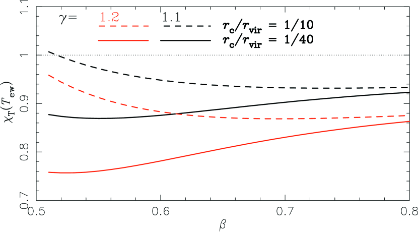
Figure 1: The bias of $H_{0}$ due to the temperature profile (eq.26) as a function of $\beta$. Dashed and solid curves correspond to the cases that core radius is 10 percent and 2.5 percent of the virial radius, respectively. Red and black colors indicate the polytropic index $\gamma=1.2$ and $1.1$, respectively.

4 Numerical modeling of systematic errors of $H_{0}$ for inhomogeneous and triaxial clusters

So far we have only considered spherical clusters. Asphericity is definitely another important source of error in the estimate of $H_{0}$. The errors are expected to be significantly reduced by averaging over a statistical sample of clusters randomly oriented with respect to our line-of-sight. Nevertheless, if clusters preferentially take either prolate or oblate shapes, for instance, the residual errors may not be entirely negligible. This is why we address the effect of asphericity on the basis of the triaxial approximation for the cluster ICM (Hughes & Birkinshaw, 1998; Jing & Suto, 2002; Lee & Suto, 2003, 2004).

To investigate quantitatively the combined effects of gas inhomogeneity and asphericity, we numerically create three sets of cluster samples and perform mock observations of Monte-Carlo realizations. The first one is spherical, but include random gas density and temperature fluctuations according to the log-normal distribution. The second one is triaxial without the fluctuations. Both the first and the second samples assume isothermality ($\gamma=1$). The third one corresponds to the model described in §3 except for added asphericity; the log-normal fluctuations, the polytropic temperature structure, and the triaxiality are included. We call them model clusters in order to distinguish them from simulated clusters extracted from cosmological hydrodynamic simulations (§5).

Each model cluster is constructed on $(512)^{3}$ grid points within 6 $\mathrm{h^{-1}Mpc}$ cubic region around the center. We first create spherically symmetric clusters with the gas density profile following equation (1) with $\beta=0.65$, $r_{\rm c}=100\mathrm{h^{-1}kpc}$, and $n_{0}=10^{-2}\mathrm{cm^{-3}}$. The gas is fiducially isothermal with $T=5$ keV, while we also consider the case of polytropic temperature profile with $T_{0}=7$ keV and $\gamma=1.2$. We then add random fluctuations of gas density and temperature according to the $r$-independent log-normal distributions. The X-ray emissivity is computed with SPEX version 2.0 assuming collisional ionization equilibrium, the energy range of $0.5-10.0$ keV and a constant metallicity $0.3Z_{\odot}$. Triaxial model clusters are constructed simply by stretching spherical clusters along the three axis directions by a factor of $\lambda_{a}$, $\lambda_{b}$, and $\lambda_{c}$, respectively.

In mock observations, we extract the quantities necessary to compute ${r_{{\rm c,iso}\beta}}(T_{\mathrm{cl}})$ and ${r_{{\rm c,fit}}}$ via equations (5) and (6) in the following manner. We first fit the projected profiles of $S_{\mathrm{x}}(\theta)$ with a functional form $S_{\mathrm{x}}(0)[1+(r/r_{\mathrm{c,fit,Sx}})^{2}]^{-3\beta_{\rm fit}+1/2}$ from $r=0$ to $r=\mathrm{1h^{-1}Mpc}$ over 1024 random LOSs toward each cluster. For each LOS, we also compute $y(0)$ and, unless otherwise stated, use it directly in our analysis. We will discuss other choices of obtaining $y(0)$ in §5.3. As will be described later, the gas temperature $T_{\rm cl}$ is obtained by either fitting the mock X-ray spectra or simply using the input temperature, depending on the purpose of the analysis. We use the template of the spectral energy distribution computed using SPEX 2.0 assuming collisional ionization equilibrium, the energy range of $0.5-10.0\mathrm{keV}$ and a constant metallicity $0.3Z_{\odot}$. Assuming that $r_{\scriptscriptstyle\parallel}={r_{{\rm c,iso}\beta}}(T_{\mathrm{cl}})$ and $r_{\scriptscriptstyle\perp}=r_{\mathrm{c,fit,Sx}}$, we calculate $f_{\scriptscriptstyle H}$ for each LOS.

To quantify the bias due to the projection effect, we also compute the volume-averaged radial profile of the gas density, directly from the grid data within the radius $\mathrm{1h^{-1}Mpc}$. By fitting the profile to the $\beta$ model, we obtain the estimated core radius $r_{\mathrm{c,fit,3D}}$, which is independent of LOS. We will compare the values of $f_{\scriptscriptstyle H}$ using $r_{\scriptscriptstyle\perp}=r_{\mathrm{c,fit,3D}}$ and $r_{\mathrm{c,fit,Sx}}$ in what follows.

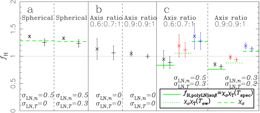
Figure 2: The average and rms of $f_{\scriptscriptstyle H}$ of the model clusters; (a) spherical clusters with gas inhomogeneities and no temperature gradient, (b) ellipsoidal and isothermal clusters, and (c) ellipsoidal clusters with temperature gradient and gas inhomogeneities. Crosses and pluses denote $f_{\scriptscriptstyle H}$ adopting $r_{\scriptscriptstyle\perp}=r_{\mathrm{c,fit,Sx}}$ and $r_{\scriptscriptstyle\perp}=r_{\mathrm{c,fit,3D}}$, respectively. Thick horizontal lines indicate analytical estimations for $\chi_{\sigma}$ (dashed), $\chi_{\sigma}\chi_{\rm T}(T_{\rm ew})$ (dotted), and $\chi_{\sigma}\chi_{\rm T}(T_{\rm spec})$ (solid). In panel (c), black symbols indicate $f_{\scriptscriptstyle H}$ using ${r_{{\rm c,iso}\beta}}(T_{\mathrm{cl}}=T_{\mathrm{spec}})$, red symbols ${r_{{\rm c,iso}\beta}}(T_{\mathrm{cl}}=T_{\mathrm{ew}})$, and blue symbols $r_{{\rm c,poly}\beta}$, which correspond to the isothermal fit with $T=T_{\rm spec}$, the isothermal fit with $T=T_{\rm ew}$, and the polytropic fit, respectively (see the main text for details).

Figure 2a shows the mean and rms values of $f_{\scriptscriptstyle H}$ for spherical clusters with no temperature gradient. We consider two cases for the log-normal density and temperature fluctuations with $(\sigma_{\mathrm{LN},\,n},\sigma_{\mathrm{LN},\,T})=(0.5,0.0)$ and $(0.5,0.3)$. The latter set corresponds to the typical value for the simulated cluster as Paper I reported. To present the bias produced solely by gas inhomogeneities, we here adopt for $T_{\mathrm{cl}}$ the volume averaged temperature instead of fitting the mock X-ray spectra. It is evident that the fluctuations in gas density yield $f_{\scriptscriptstyle H}\sim 1.3$ (i.e. overestimating of $H_{0}$ by $\sim 30\%$), while those in gas temperature do not contribute significantly to the bias. The mean value of $f_{\scriptscriptstyle H}$ is in good agreement with our analytical expectation $\chi_{\sigma}$ (dashed horizontal lines). The bias due to the projection is $\sim 10\%$.

The bias produced by ellipsoidal shapes is displayed in Figure 2b for the two sets of the axis ratio ($\lambda_{a}:\lambda_{b}:\lambda_{c}=0.6:0.7:1$ and $0.9:0.9:1$). These sets are the typical value of the simulated cluster. Again, to present the bias solely from asphericity, the gas is assumed to be isothermal without any fluctuations and we adopt $T_{\mathrm{cl}}=T_{0}$ in computing $f_{\scriptscriptstyle H}$. The average bias is relatively small ($\lesssim 15\%$) and that due to the projection is $\sim 3\%$. These results indicate that the bias due to asphericity, after averaging over a statistical sample of clusters, is smaller than that from gas inhomogeneity.

Figure 2c illustrates the bias in a more realistic case; we create ellipsoidal clusters with the polytropic temperature profile and fluctuations. Two sets of axis ratio ($\lambda_{a}:\lambda_{b}:\lambda_{c}=0.6:0.7:1$ and $0.9:0.9:1$) are chosen adopting $(\sigma_{\mathrm{LN},\,n},\sigma_{\mathrm{LN},\,T})=(0.5,0.3)$ and $(0.3,0.2)$, respectively. In this panel, we show the values of $f_{\scriptscriptstyle H}$ based on the following three methods, so as to understand clearly the physical origin of the overall bias in the $H_{0}$ estimation.

The first method (black symbols in Fig. 2c) corresponds to the most conventional case of using the isothermal $\beta$-model and the spectroscopic temperature $T_{\rm spec}$. To obtain $T_{\rm spec}$ we fit the mock X-ray spectra from the central ($r<1$ $\mathrm{h^{-1}Mpc}$) region of each cluster using XSPEC assuming a single temperature MEKAL model. We assume the perfect response, and ignore its effect on the spectral temperature (Paper I). Clearly, the value of $H_{0}$ is underestimated by $\sim 10$-$20\%$. This is in good agreement with our analytical estimation for $f_{\rm H,polyLN|iso\beta}=\chi_{\sigma}\chi_{\rm T}(T_{\rm spec})$ for a spherical cluster (solid horizontal lines). To obtain $\chi_{\rm T}(T_{\mathrm{spec}})$, we compute the volume-averaged profile of the density and the temperature. These profile are fitted to equation (1) and equation (14) taking $n_{0}$, $r_{\mathrm{c,fit,3D}}$, $\beta$, $T_{0}$ and $\gamma$ as free parameters. We use the adopted values $(\sigma_{\mathrm{LN},\,n},\sigma_{\mathrm{LN},\,T})=(0.5,0.3)$ and $(0.3,0.2)$ to compute $\chi_{\sigma}$.

The second method (red symbols in Fig. 2c) aims to mimic previous numerical studies of the $H_{0}$ bias (Inagaki, Suginohara & Suto, 1995; Yoshikawa, Itoh & Suto, 1998) and adopts the isothermal $\beta$-model and the emission-weighted temperature $T_{\rm ew}$. We obtain $T_{\mathrm{ew}}$ by directly summing up the temperature of each grid point from the central ($r<1$ $\mathrm{h^{-1}Mpc}$) region. Also plotted for comparison is an analytical estimate $\chi_{\sigma}\chi_{\rm T}(T_{\rm ew})$ (dotted lines). The values of $\chi_{\sigma}$ and $\chi_{\rm T}(T_{\rm ew})$ are computed as described above. In this case, $\chi_{\sigma}$ and $\chi_{\rm T}(T_{\rm ew})$practically cancel each other, and $f_{\scriptscriptstyle H}$ is close to unity, consistent with the previous findings of Inagaki, Suginohara & Suto (1995) and Yoshikawa, Itoh & Suto (1998). This shows that the absence of the bias in previous studies is simply an artifact of using $T_{\mathrm{ew}}$, which is systematically larger than $T_{\rm spec}$.

The third method (blue symbols in Fig. 2c) attempts to eliminate the bias due to the temperature gradient by using the polytropic profile to estimate the core radius (Ameglio et al., 2006) :

$$r_{{\rm c,poly}\beta} = \frac{y(0)^{2}}{S_{\mathrm{x}}(0)}\frac{m_{e}^{2}c^{4}\Lambda_{\rm x}(T_{0})}{4\pi(\sigma_{\mathrm{T}}kT_{0})^{2}(1+z)^{4}}\frac{G(\beta\gamma/4+3\beta/4)}{[G(\beta\gamma/2)]^{2}},$$ (29)

where we adopt $T_{0}$ and $\gamma$ from fitting the volume-averaged temperature profile of the model clusters. The value of $\beta$ is obtained from equation (19) using $\beta_{\rm fit}$ and $\gamma$. The value of $f_{\scriptscriptstyle H}$ so obtained should represent the bias arising from sources other than the spectral fitting and the temperature gradient. Given the good agreement with the analytical estimate for $\chi_{\sigma}$ (dashed lines), we conclude that the bias in this case is dominated by the effect from gas inhomogeneities.

In summary, there are three major sources for the bias of $H_{0}$; the spectral fitting, the temperature gradient, and local density fluctuations. The former two leads to an underestimate while the latter an overestimate of $H_{0}$. In every case studied here, the bias due to asphericity is much smaller than the other three.

5 Comparison with clusters from cosmological hydrodynamic simulations

5.1 Cosmological hydrodynamic simulations

We now compare the bias described in the previous section with simulated clusters. They are extracted from the Smoothing Particle Hydrodynamic (SPH) simulation of the local universe performed by Dolag et al. (2005) assuming $\Lambda$CDM universe with $\Omega_{0m}=0.3,\Omega_{b}=0.04,\sigma_{8}=0.9$, and $h=0.7$. The numbers of dark matter and SPH particles are $\sim 20$ million each within a high-resolution sphere of radius $\sim 110Mpc$, which is embedded in a periodic box $\sim 343$ Mpc on a side that is filled with nearly 7 million low-resolution dark matter particles. The simulation is designed to reproduce the matter distribution of the local universe adopting the initial conditions based on the IRAS galaxy distribution, smoothed over a scale of $4.9h^{-1}\mathrm{Mpc}$. We choose the six massive clusters identified as Coma, Perseus, Virgo, Centaurus, A3627, and Hydra. Figure 3 shows projected surface density maps of these simulated clusters. The values of $\beta$ and $\gamma$ of these clusters are listed in Table 1. The cubic region of 6 $h^{-1}$ Mpc around the center of each cluster is extracted and divided into $512^{3}$ cells. The density and temperature of each mesh point are calculated from SPH particles using the B-spline smoothing kernel. A detailed description of this procedure is given in Paper I.

We perform mock observations over 1024 LOSs for each simulated cluster in a similar manner to §4 except for the following points. First, we compute $T_{\mathrm{spec}}$ and $T_{\mathrm{ew}}$ within the virial radius instead of 1 $\mathrm{h^{-1}Mpc}$. Second, we use the fitted value of $\sigma_{\mathrm{LN},\,n}$ and $\sigma_{\mathrm{LN},\,T}$ in calculating $\chi_{\sigma}$ of the analytical model.

Table 1: Properties of the Six Simulated Clusters.

	$\beta_{\mathrm{fit,3D}}$ $\,{}^{*}$	$\gamma$ $\,{}^{*}$	$\lambda_{a}/\lambda_{c}$	$\lambda_{b}/\lambda_{c}$	$\langle r_{\mathrm{c,fit,Sx}}\rangle/r_{\mathrm{c,fit,3D}}$
Coma	0.74	1.17	0.59	0.64	1.03 $\pm$ 0.14
Perseus	0.64	1.09	0.49	0.61	1.04 $\pm$ 0.18
Virgo	0.60	1.15	0.44	0.61	1.16 $\pm$ 0.31
Centaurus	0.69	1.17	0.68	0.78	1.03 $\pm$ 0.13
A3627	0.69	1.15	0.79	0.83	1.08 $\pm$ 0.06
Hydra	0.70	1.22	0.84	0.93	1.03 $\pm$ 0.05
$\ast$ The values of $\beta_{\mathrm{fit,3D}}$ and $\gamma$ are slightly changed from that listed in Paper I due to the improvement of the routine of fits.

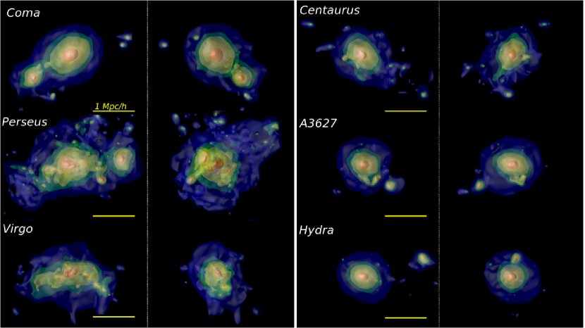
Figure 3: Projected surface density maps of the six simulated clusters. Five different ($n_{e}=3\times 10^{-3},1\times 10^{-3},5\times 10^{-4},3\times 10^{-4}$, and $1\times 10^{-4}$ [$\mathrm{cm^{-3}}$]) isodensity surfaces are indicated with different colors (red, orange, yellow, green, and blue, respectively). The left panels of each cluster indicate the view from our galaxy. The right panels are the projection of each simulated cluster as seen by a distant observer located to the “right” of each panel on the left. The horizontal yellow lines indicate the physical size of $1\,\mathrm{h^{-1}Mpc}$.

5.2 Results

Figure 4 displays a set of histograms of $f_{\scriptscriptstyle H}$ for the simulated Coma cluster. The same analysis is done for the other five clusters. Histograms in different colors correspond to the symbols of the same color in Figure 2c, and indeed show similar trends for each component of the bias. Since the physical length of clusters along the LOS is not symmetrically distributed around its mean, the corresponding histograms of $f_{\scriptscriptstyle H}$ are skewed positively. In Appendix A, we compute the distribution for the two extreme cases, the prolate and the oblate ellipsoids, and find that they yield positively and negatively skewed distributions, respectively. Indeed this is consistent with the fact that the simulated Coma is nearly prolate (Table 1) .

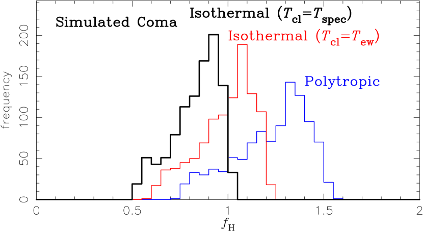
Figure 4: Distribution of $f_{\scriptscriptstyle H}$ over 1024 LOSs for the simulated Coma cluster. Black, red and blue histograms indicate the results for the isothermal fit with $T=T_{\rm spec}$, the isothermal fit with $T=T_{\rm ew}$, and the polytropic fit, respectively.

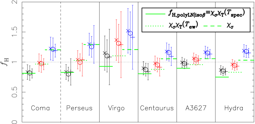
Figure 5: The average and rms of $f_{\scriptscriptstyle H}$ for the six simulated clusters. Black, red and blue symbols with error-bars indicate the results for the isothermal fit with $T=T_{\rm spec}$, the isothermal fit with $T=T_{\rm ew}$, and the polytropic fit, respectively. Crosses and pluses denote $f_{\scriptscriptstyle H}$ adopting $r_{\scriptscriptstyle\perp}=r_{\mathrm{c,fit,Sx}}$ and $r_{\scriptscriptstyle\perp}=r_{\mathrm{c,fit,3D}}$, respectively. Open circles indicate $f_{\scriptscriptstyle H}$ adopting $r_{\scriptscriptstyle\perp}=r_{\mathrm{c,fit,Sx}}$ but assuming that the clusters are not extended beyond the virial radius. Thick green horizontal lines indicate analytical estimations for $\chi_{\sigma}$ (dashed), $\chi_{\sigma}\chi_{\rm T}(T_{\rm ew})$ (dotted), and $\chi_{\sigma}\chi_{\rm T}(T_{\rm spec})$ (solid).

The (simple arithmetic) mean, $\langle f_{\scriptscriptstyle H}\rangle$ is plotted in Figure 5 for six simulated clusters. The quoted error bars indicate 1$\sigma$ standard deviation from the mean. Except for the simulated Virgo cluster, $\langle f_{\scriptscriptstyle H}\rangle$ is below unity, i.e., $H_{0}$ is underestimated. It is remarkable that a simple analytical model for systematic effects (solid, dotted and dashed horizontal lines) described in §3 can reproduce the bias in the simulated clusters.

We have made sure that the bias from other sources is minor; first, if a cluster has a finite extension and is bounded within the virial radius, the value of $\langle f_{\scriptscriptstyle H}\rangle$ becomes smaller by $\lesssim 5\%$ (open circles in Fig. 5). Second, we compute the axis ratio ($\lambda_{a}<\lambda_{b}<\lambda_{c}$) of each simulated cluster, basically following the method of Jing & Suto (2002), but using the gas density not the dark matter density. The isodensity surfaces corresponding to the gas densities of $n_{e}=3\times 10^{-3}$, $1\times 10^{-3}$, $5\times 10^{-4}$, $3\times 10^{-4}$, and $1\times 10^{-4}$ [$\mathrm{cm^{-3}}$] are shown in Figure 3. After eliminating substructures, the axis ratio is calculated by diagonalizing the inertial tensor of each surface. The averaged axis ratios of the five different density regions (Table 1) are similar to the typical value adopted in §4. Therefore, we conclude that the spherical approximation itself is not a major source of the bias for the simulated cluster. Finally, the bias due to the projection is small (crosses and pluses in Fig. 5). We list in Table 1 the average values of $r_{\mathrm{c,fit,Sx}}$ over 1024 LOSs relative to $r_{\mathrm{c,fit,3D}}$. The ratio is unity within 10 % (except for Virgo that has a relatively large dispersion), and basically all consistent with unity within the uncertainty.

It is interesting to emphasize here that the shape of the distribution of $f_{\scriptscriptstyle H}$ reflects the shape of clusters from the perspective of measuring the three-dimensional shape of clusters (Sereno et al., 2006, e.g.). If all clusters had the same shape, the observation of one cluster toward multiple directions might correspond to that of multiple clusters toward each LOS. Of course, the real shapes vary from cluster to cluster. However, if clusters tend to be prolate (oblate) preferentially, the distribution of $H_{\rm 0,est}$ should be skewed positively (negatively) as shown in appendix A. Therefore, independently of the knowledge of real value of $H_{\rm 0,true}$, the statistical information about the shape distribution may be obtained in principle by the distribution of $H_{\rm 0,est}$.

5.3 Comparison with previous studies

The above results are consistent with the previous results of $f_{\scriptscriptstyle H}\sim 1$ with $T_{\mathrm{cl}}=T_{\mathrm{ew}}$ (Inagaki, Suginohara & Suto, 1995; Yoshikawa, Itoh & Suto, 1998). On the other hand, Ameglio et al. (2006) explored the bias of $d_{\mathrm{A}}$ using the cosmological hydrodynamic simulations, and reported that $H_{0}$ is overestimated by more than a factor of two if one adopts the isothermal $\beta$ model. This is opposite to our conclusion here, and we found that this should be ascribed to the sensitivity of $f_{\rm H}$ on the adopted values of $y(0)$, i.e., $f_{\rm H}\propto d_{\mathrm{A,est}}^{-1}\propto y^{-2}(0)$ as explained below.

Ameglio et al. (2006) obtained $y(0)$ by fitting the noise-less profile of $y(\theta)$ up to $R_{500}$ fixing other $\beta$-model parameters from the X-ray profile, while we use directly the projected values of $y(0)$ in the simulation data. The difference in these two methods is apparent in Figure 5 (right panel) of Ameglio et al. (2006); their fit (solid line) was affected largely by the data points at large radii and yielded a value of $y(0)$ smaller by $\sim 50\%$ than the actual data. This enhances the value of $f_{\rm H}$ by more than a factor of two, and indeed accounts for their apparently opposite conclusions. We have checked that other differences between their analysis and ours (the use of mass-weighted temperature for $T_{\mathrm{cl}}$ and the removal of the cluster central region) do not affect the results significantly.

As far as the bias in the previous SZE observations is concerned, we believe that our method is more relevant to what has been done with the real data, because these observations were not capable of constraining the radial profile of the y-parameter up to large radii with high S/N (see Komatsu et al., 2001; Kitayama et al., 2004, for the currently highest angular-resolution observation of the SZE).

We have further made sure that the effects of the finite spatial resolution of the observations and the central cooling region, which were neglected in our preceding analysis, are minor; first, we have evaluated $y(0)$ by fitting $y(\theta)$ within a radius of 100 $h^{-1}\mathrm{kpc}$ and 200 $h^{-1}\mathrm{kpc}$. These approximately correspond to the typical angular resolution of the SZE observation ($\sim$ 1 minute) at $z=0.1$ and $z=0.3$, respectively. The values of $\beta$ and $\theta_{c}$ are fixed from the X-ray profile. For the six simulated clusters, the resulting values of $f_{\rm H}$ differ from our initial analysis (see Fig. 5) by $-6\%$ to $+7\%$ ($+2\%$ on average) for $r<100h^{-1}\mathrm{kpc}$, and by $-3\%$ to $+10\%$ ($+5\%$ on average) for $r<200h^{-1}\mathrm{kpc}$.

Second, we have also performed the fitting separately for the X-ray and SZE profiles. The values of $S_{\mathrm{x}}$, $\beta$ and $\theta_{c}$ are evaluated by fitting $S_{\mathrm{x}}(\theta)$ with equation (2), while that of $y(0)$ is obtained by fitting $y(\theta)$ with equation (3) independently of the X-ray profile. As a result, the values of $f_{\rm H}$ differ from those of Figure 5 by $-6\%$ and $+1\%$ ($-3\%$ on average).

Note that observationally there are several different ways to evaluate $y(0)$, $S_{\mathrm{x}}(0)$, $\beta$ and $\theta_{c}$. A conventional method is to fit the X-ray imaging data $S_{\mathrm{x}}(\theta)$ first. Then the SZ image is fitted to obtain $y(0)$ assuming the values of $\beta$ and $\theta_{c}$ from the X-ray data. Our analysis procedure adopted here follows the conventional method. While Reese et al. (2002) have determined $d_{A}$ from the joint fit to the X-ray and SZE imaging data, the result is almost equivalent to the conventional method since the X-ray imaging data have a much higher S/N than the SZE data.

6 Conclusions

We considered various possible systematic errors of $H_{0}$ from the combined analysis of the Sunyaev-Zel’dovich effect and X-ray observations. In particular we addressed the validity and limitation of the spherical isothermal $\beta$ model in estimating $H_{0}$, which has been used widely as a reasonable approximation after averaging over a number of clusters. We introduced the ratio of the estimated to the true Hubble constant, $f_{H}$, to characterize the systematic errors. We constructed an analytic model for $f_{H}$, and identified three important sources for the systematic errors; density and temperature inhomogeneities in the ICM, the temperature profile, and departures from sphericity. Except for the non-spherical effect, the most important analytical expression that summarizes our conclusion is equation (23), or equivalently,

$$\frac{H_{\rm 0,est}}{H_{\rm 0,true}}=\chi_{\sigma}~{}\chi_{\rm T}(T_{\mathrm{ew}})~{}\chi_{\rm spec-ew}.$$ (30)

In our analytic model discussed in §3, the inhomogeneity bias, $\chi_{\sigma}$, the non-isothermality bias, $\chi_{\rm T}(T_{\mathrm{ew}})$, and the temperature bias $\chi_{\rm spec-ew}$ are given by equations (13), (26), and (28), respectively.

While the above model prediction is fairly general, the net value of $f_{\rm H}$ sensitively depends on the degree of the inhomogeneity and multi-phase temperature structure of real ICM. Our simulated cluster sample implies that $\chi_{\sigma}\approx(1.1-1.3)$, $\chi_{\rm T}(T_{\mathrm{ew}})\approx(0.8-1)$, $\chi_{\rm spec-ew}\approx(0.8-0.9)$, and therefore $\langle f_{\rm H}\rangle\approx(0.8-0.9)$. Given the result of Reese et al. (2002), this is certainly indicative, but may need to be interpreted with caution because the result is critically dependent on the reliability of the adopted numerically simulated clusters as representative samples of clusters observed in the real universe. Exactly for this reason, we are attempting more direct (not statistical) comparison of our model prediction against observed cluster samples, which will be presented elsewhere hopefully in the near future (Reese et al. in preparation).

We thank Noriko Yamasaki and Kazuhisa Mitsuda for useful discussions, Klaus Dolag for providing a set of simulated cluster samples, and Erik Reese for a careful reading of the manuscript. We also thank an anonymous referee for several constructive comments. The simulations were performed at the Data-Reservoir at the University of Tokyo, and we thank Mary Inaba and Kei Hiraki for providing the computational resources. This work is supported by Grant-in-Aid for Scientific research of Japanese Ministry of Education, Culture, Sports, Science and Technology (Nos. 14102204, 15740157, 16340053, 18740112, and 18072002), and by JSPS (Japan Society for Promotion of Science) Core-to-Core Program “International Research Network for Dark Energy”.

Appendix A Distribution of $f_{\scriptscriptstyle H}$ for prolate and oblate ellipsoids

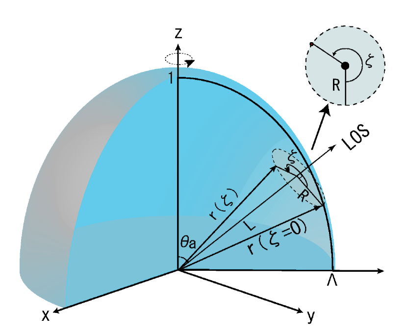
Figure 6: Schematic representation of a prolate cluster with an axis ratio $\lambda_{a}:\lambda_{b}:\lambda_{c}=1:\Lambda:\Lambda$. Given the symmetry around the $z$-axis (the long axis), an LOS through the cluster center is specified by an angle $\theta_{{\bf a}}$ from the $z$-axis. An arbitrary position in the cluster ${\bf r}$ is expressed in terms of $L$ (the projection of ${\bf r}$ onto the LOS direction), $R$ (the projection of ${\bf r}$ onto the plane normal to the LOS), and $\zeta$ (the azimuthal angle on the plane normal to the LOS).

In this Appendix, we derive the distribution of $f_{\scriptscriptstyle H}$ due to the asphericity of clusters, by considering the following two extreme cases; the prolate ($\lambda_{a}=\lambda_{b}<\lambda_{c}$) and the oblate ($\lambda_{a}<\lambda_{b}=\lambda_{c}$) ellipsoids. We choose $z$-axis as the long (short) axis and $x$- and $y$-axes as the short (long) axes for an prolate (oblate) ellipsoid. The direction of the unit vector along the LOS of an observer, ${\bf a}$, is defined in terms of the spherical coordinate ($\theta_{{\bf a}}$, $\phi_{{\bf a}}$). Figure 6 shows a schematic picture of a prolate ellipsoid.

Let us define the quantity $\Lambda\equiv\lambda_{a}/\lambda_{c}=\lambda_{b}/\lambda_{c}$ ($\Lambda\equiv\lambda_{b}/\lambda_{a}=\lambda_{c}/\lambda_{a}$) for the prolate (oblate) ellipsoid. We assume that the gas density follows the prolate (oblate) $\beta$ model:

$$n({\bf r})_{|\theta_{{\bf a}}} = n_{0}\left(1+(\tilde{r}/r_{\mathrm{c}})^{2}\right)^{-3\beta/2},$$ (A1)

$$\tilde{r} \equiv |{\bf r}|[\sin^{2}{\theta_{{\bf r}}}/\Lambda^{2}+\cos^{2}{\theta_{{\bf r}}}]^{1/2},$$ (A2)

and $\theta_{{\bf r}}$ is the angle between $z$-axis and ${\bf r}$. Because the surface brightness profile is independent of $\phi_{{\bf a}}$ due to the $z$-axial symmetry, one can express $f_{\scriptscriptstyle H}$ as function of $\theta_{{\bf a}}$.

For an isothermal cluster, the surface brightness averaged over a circle of radius $R$ is proportional to $\int n^{2}dL$ averaged over the angle $\zeta$ of the circle. We put $\zeta=0$ where ${\bf r}$ is located on the same plane defined by the LOS and $z$-axis. To compute the averaged surface brightness, we need an expression of the density $n$ as a function of $L$, $R$, and $\zeta$. In the Cartesian coordinate, ${\bf r}(\zeta=0)$ is

$${\bf r}(\zeta=0)=\left(\begin{array}[]{rl}\sqrt{R^{2}+L^{2}}\cos{\phi_{{\bf a}}}\sin{(\arctan{R/L}+\theta_{{\bf a}})}\\ \sqrt{R^{2}+L^{2}}\sin{\phi_{{\bf a}}}\sin{(\arctan{R/L}+\theta_{{\bf a}})}\\ \sqrt{R^{2}+L^{2}}\cos{(\arctan{R/L}+\theta_{{\bf a}})}\end{array}\right).$$ (A6)

Multiplying the rotation matrix around ${\bf a}$, ${\it M}_{{\bf a}}(\zeta)$ to ${\bf r}(\zeta=0)$, we obtain

$${\bf r}(\zeta) = {\it M}_{{\bf a}}(\zeta){\bf r}(\zeta=0)$$ (A7)

$$= \left(\begin{array}[]{rl}R\cos{\zeta}\cos{\phi_{{\bf a}}}\cos{\theta_{{\bf a}}}+R\sin{\zeta}\sin{\phi_{{\bf a}}}+L\cos{\phi_{{\bf a}}}\sin{\theta_{{\bf a}}}\\ R\cos{\zeta}\sin{\phi_{{\bf a}}}\cos{\theta_{{\bf a}}}-R\sin{\zeta}\cos{\phi_{{\bf a}}}+L\sin{\phi_{{\bf a}}}\sin{\theta_{{\bf a}}}\\ L\cos{\theta_{{\bf a}}}-R\cos{\zeta}\sin{\theta_{{\bf a}}}\end{array}\right),$$ (A11)

where

$${\it M}_{{\bf a}}(\zeta)\equiv$$ (A12)

$$\left(\begin{array}[]{ccc}x_{\bf a}^{2}+(1-x_{\bf a}^{2})\cos{\zeta}&x_{\bf a}y_{\bf a}(1-\cos{\zeta})+z_{\bf a}\sin{\zeta}&z_{\bf a}x_{\bf a}(1-\cos{\zeta})-y_{\bf a}\sin{\zeta}\\ x_{\bf a}y_{\bf a}(1-\cos{\zeta})-z_{\bf a}\sin{\zeta}&y_{\bf a}^{2}+(1-y_{\bf a}^{2})\cos{\zeta}&y_{\bf a}z_{\bf a}(1-\cos{\zeta})+x_{\bf a}\sin{\zeta}\\ z_{\bf a}x_{\bf a}(1-\cos{\zeta})+y_{\bf a}\sin{\zeta}&y_{\bf a}z_{\bf a}(1-\cos{\zeta})-x_{\bf a}\sin{\zeta}&z_{\bf a}^{2}+(1-z_{\bf a}^{2})\cos{\zeta}\end{array}\right),$$ (A16)

and

$$\left(\begin{array}[]{rl}x_{\bf a}\\ y_{\bf a}\\ z_{\bf a}\end{array}\right)\equiv\left(\begin{array}[]{rl}\cos{\phi_{{\bf a}}}\sin{\theta_{{\bf a}}}\\ \sin{\phi_{{\bf a}}}\sin{\theta_{{\bf a}}}\\ \cos{\theta_{{\bf a}}}\end{array}\right).$$ (A23)

Thus, we obtain

$$|{\bf r}(\zeta)|\cos{\theta_{{\bf r}}}=L\cos{\theta_{{\bf a}}}-R\cos{\zeta}\sin{\theta_{{\bf a}}}.$$ (A24)

Then, $|{\bf r}(\zeta)|$ and $\theta_{{\bf r}}$ are written as

$$|{\bf r}(\zeta)| = \sqrt{L^{2}+R^{2}}$$ (A25)

$$\theta_{{\bf r}} = \arccos{\left(\frac{L\cos{\theta_{{\bf a}}}-R\cos{\zeta}\sin{\theta_{{\bf a}}}}{\sqrt{L^{2}+R^{2}}}\right)}.$$ (A26)

Combining with equation (A1), we can write $n({\bf r})_{|\theta_{{\bf a}}}$ in terms of $L$,$R$, and $\zeta$ as

$$n({\bf r})_{|\theta_{{\bf a}}}=n_{0}\left(1+(\tilde{r}(R,L,\zeta)_{|\theta_{{\bf a}}}/r_{\mathrm{c}})^{2}\right)^{-3\beta/2}\equiv n(R,L,\zeta),$$ (A27)

where

$$\tilde{r}(R,L,\zeta)_{|\theta_{{\bf a}}}\equiv\tilde{r}=\frac{\sqrt{L^{2}+R^{2}+[\Lambda^{2}-1](L\cos{\theta_{{\bf a}}}-R\cos{\zeta}\sin{\theta_{{\bf a}}})^{2}}}{\Lambda}.$$ (A28)

Then, the averaged surface brightness at $R$ is

$$S_{\mathrm{x}}(R)_{|\theta_{{\bf a}}} = \frac{1}{2\pi}\int_{0}^{2\pi}d\zeta\int_{-\infty}^{\infty}dL[n(R,L,\zeta)_{|\theta_{{\bf a}}}]^{2}$$ (A29)

$$= \frac{n_{0}^{2}r_{\mathrm{c}}}{2\pi}\int_{0}^{2\pi}d\zeta\int_{-\infty}^{\infty}dq_{L}\left[\frac{q_{L}^{2}+q_{R}^{2}+(\Lambda^{2}-1)(q_{L}\cos{\theta_{{\bf a}}}-q_{R}\cos{\zeta}\sin{\theta_{{\bf a}}})^{2}}{\Lambda^{2}}+1\right]^{-3\beta}$$ (A30)

$$\equiv \frac{n_{0}^{2}r_{\mathrm{c}}}{2\pi}I(q_{R})_{|\theta_{{\bf a}}}$$ (A31)

where we define the normalized length by $r_{\mathrm{c}}$, $q_{R}\equiv R/r_{\mathrm{c}}$,$q_{L}\equiv L/r_{\mathrm{c}}$. We compute $I(q_{R})_{|\theta_{{\bf a}}}$ numerically for $\Lambda=0.5$ (prolate) and $\Lambda=2.0$ (oblate) adopting $\beta=0.65$. We fit $I(q_{R})_{|\theta_{{\bf a}}}$ from $q_{R}=0$ to $q_{R}=10.0$ by with a functional form of the surface brightness profile assuming the spherical beta model $(\propto[1+(q_{R}/q_{c,\mathrm{fit}|\theta_{{\bf a}}})^{2}]^{-3\beta_{\mathrm{fit}|\theta_{{\bf a}}}+1/2})$. Thus, we obtain the counter part of ${r_{{\rm c,iso}\beta}}$ , $q_{c,\mathrm{fit}|\theta_{{\bf a}}}\equiv r_{\mathrm{c,fit,Sx}}/r_{\mathrm{c}}$ and the fitted value of $\beta$, $\beta_{\mathrm{fit}|\theta_{{\bf a}}}$. While, $q_{\rm c,iso\beta|\theta_{{\bf a}}}\equiv{r_{{\rm c,iso}\beta}}/r_{\mathrm{c}}$ is written as

$$q_{\rm c,iso\beta|\theta_{{\bf a}}}=(\sin^{2}{\theta_{{\bf a}}}/\Lambda^{2}+\cos^{2}{\theta_{{\bf a}}})^{-1/2}\frac{G(\beta)G(\beta_{\mathrm{fit}|\theta_{{\bf a}}}/2)^{2}}{G(\beta/2)^{2}G(\beta_{\mathrm{fit}|\theta_{{\bf a}}})}.$$ (A32)

The first term of the right-hand side represents the elongation of the radius toward the LOS. The second term is the correction to the use of $\beta_{\mathrm{fit}|\theta_{{\bf a}}}$ in observation instead of the true $\beta$. However, the correction is very small (within 0.01% error).

Finally, we obtain the bias of $H_{0}$ as a function of $\theta_{{\bf a}}$,

$$f_{\scriptscriptstyle H}(\theta_{{\bf a}})\equiv\frac{q_{\mathrm{c,\mathrm{fit}|\theta_{{\bf a}}}}}{q_{\rm c,iso\beta|\theta_{{\bf a}}}}.$$ (A33)

The probability of $f_{\scriptscriptstyle H}$ for the random assignment is proportional to the solid angle $\Omega(f_{\scriptscriptstyle H})$. If $f_{\scriptscriptstyle H}(\theta_{{\bf a}})$ is a monotonic function, the PDF of $f_{\scriptscriptstyle H}$ is obtained as

$$P(f_{\scriptscriptstyle H})=\frac{1}{4\pi}\frac{d\Omega}{df_{\scriptscriptstyle H}} = \frac{1}{4\pi}\frac{d\Omega}{d\theta_{{\bf a}}}\Big{|}\frac{d\theta_{{\bf a}}}{df_{\scriptscriptstyle H}}\Big{|}$$ (A34)

$$= \frac{\sin{\theta_{{\bf a}}(f_{\scriptscriptstyle H})}}{2}\Big{|}\frac{d\theta_{{\bf a}}(f_{\scriptscriptstyle H})}{df_{\scriptscriptstyle H}}\Big{|},$$ (A35)

where $\theta_{{\bf a}}(f_{\scriptscriptstyle H})=f^{-1}_{{\scriptscriptstyle H}}(\theta_{{\bf a}})$.

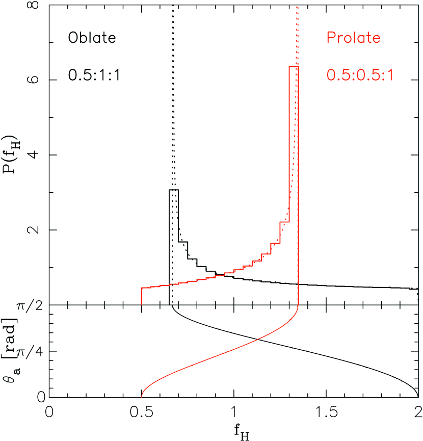
Figure 7: Upper: The PDF of $f_{\scriptscriptstyle H}$ for the oblate ($\Lambda=2$; black curves) and prolate ($\lambda=0.5$; red curves) ellipsoids. Dotted lines represent equation (A34), while solid lines show the corresponding histograms with a bin size of $\Delta f_{\scriptscriptstyle H}=0.05$. Lower: The angle, $\theta_{{\bf a}}$, as a function of $f_{\scriptscriptstyle H}$.

Dotted lines in the upper panel of Figure 7 show equation (A34) for prolate ($\Lambda=0.5$) and oblate ($\Lambda=2.0$) ellipsoids. As shown in the lower panel, the corresponding $\theta_{{\bf a}}$ is a monotonically increasing (decreasing) function of $f_{\scriptscriptstyle H}$ for the prolate (oblate) ellipsoid. At $\theta_{{\bf a}}=0$, $f_{\scriptscriptstyle H}$ is equal to $\Lambda$, which corresponds to the case that the LOS is along the $z$-axis.

The PDF diverges at $\theta_{{\bf a}}=\pi/2$. This can be understood as follows. Equations (A32) to (A34) imply that

$$P(f_{\scriptscriptstyle H})\propto\sin{\theta_{{\bf a}}(f_{\scriptscriptstyle H})}\Big{|}\frac{dq_{\rm c,iso\beta|\theta_{{\bf a}}}^{-1}}{d\theta_{{\bf a}}(f_{\scriptscriptstyle H})}\Big{|}^{-1}\propto\frac{\sqrt{\cos^{2}\theta_{{\bf a}}(f_{\scriptscriptstyle H})+\Lambda^{-2}\sin^{2}\theta_{{\bf a}}(f_{\scriptscriptstyle H})}}{\cos\theta_{{\bf a}}(f_{\scriptscriptstyle H})},$$ (A36)

where we ignore the $\theta_{{\bf a}}$-dependence of $q_{c,\mathrm{fit|\theta_{{\bf a}}}}$ and $\beta_{\mathrm{fit}|\theta_{{\bf a}}}$. Thus $\theta_{{\bf a}}\approx\pi/2$, $P(f_{\scriptscriptstyle H})$ diverges as $1/\cos\theta_{{\bf a}}$. Note, however, its integration over a finite size of $f_{\scriptscriptstyle H}$ does not diverge (see eq.[A34]). This is plotted in the solid histograms, where the bin size $\Delta f_{\scriptscriptstyle H}=0.05$ is adopted. The resulting distribution is skewed positively (negatively) for the prolate (oblate) ellipsoid, which is consistent with the results shown in Figure 4.

References

• Ameglio et al. (2006) Ameglio, S., Borgani, S., Diaferio, A., & Dolag, K. 2006, MNRAS, 369, 1459
• Birkinshaw (1999) Birkinshaw, M., 1999, Physics Report, 310, 97
• Bonamente et al. (2006) Bonamente et al., 2006, ApJ, 647, 25
• Carlstrom et al. (2002) Carlstrom, J. E., Holder, G. P., and Reese, E. D. 2002, ARA&A, 40, 643
• Dolag et al. (2005) Dolag, K.,Hansen, F. K.,Roncarelli, & M.,Moscardini, L. 2005, MNRAS, 363, 29
• Freedman et al. (2001) Freedman et al., 2001, ApJ, 553, 47
• Hughes & Birkinshaw (1998) Hughes, J. P., & Birkinshaw, M. 1998, ApJ, 501, 1
• Inagaki, Suginohara & Suto (1995) Inagaki, Y., Suginohara, T., & Suto, Y. 1995, PASJ, 47, 411
• Jing & Suto (2002) Jing, Y. P., & Suto, Y. 2002, ApJ, 574, 538
• Kawahara et al. (2007) Kawahara, H., Suto, Y., Kitayama, T.,Sasaki, S., Shimizu, M, Rasia, E.,& Dolag, K. 2007, ApJ, 659, 257 (paper I)
• Kay et al. (2006) Kay, S. T. , da Silva, A. C. , Aghanim, N. , Blanchard, A. , Liddle, A. R. , Puget, J.-L. , Sadat, R. ,& Thomas, P. A, 2006, astro-ph/0611017
• Kobayashi, Sasaki & Suto (1996) Kobayashi, S., Sasaki, S., & Suto, Y. 1996, PASJ, 48, 107
• Komatsu et al. (2001) Komatsu, E., Matsuo, H., Kitayama, T., Hattori, M., Kawabe, R., Kohno, K., Kuno, N., Schindler, S., Suto, Y., & Yoshikawa, K. 2001, PASJ, 53, 57
• Kitayama et al. (2004) Kitayama, T., Komatsu, E., Ota, N., Kuwabara, T., Suto, Y., Yoshikawa, K., Hattori, M., & Matsuo, H. 2004, PASJ, 56, 17
• Lee & Suto (2003) Lee, J. & Suto, Y. 2003, ApJ, 585, 151
• Lee & Suto (2004) Lee, J. & Suto, Y. 2004, ApJ, 601, 599
• Mazzotta et al. (2004) Mazzotta, P., Rasia, E., Moscardini, L., & Tormen, G. 2004, MNRAS, 354, 10
• Rasia et al. (2005) Rasia, E., Mazzotta, P., Borgani, S., Moscardini, L., Dolag, K., Tormen, G., Diaferio, A., & Murante, G. 2005, ApJ, 618, L1
• Reese et al. (2002) Reese, E.D., Carlstrom, J.E., Joy, M., Mohr, J.J., Grego, L., & Holzapfel, W.L. 2002, ApJ, 581, 53
• Sereno et al. (2006) Sereno, M., De Filippis, E., Longo, G., & Bautz, M. W. 2006, ApJ, 645, 170
• Silk & White (1978) Silk, J. & White, S.D.M. 1978, ApJ,226,L103
• Spergel et al. (2007) Spergel et al. 2007, ApJS, 170, 377
• Sulkanen (1999) Sulkanen, M.E. 1999, ApJ, 522, 59
• Sunyaev & Zel’dovich (1972) Sunyaev R.A. & Zel’dovich Ya.B. 1972, Comments on Astrophys.& Space Phys., 4, 173
• Uzan et al. (2004) Uzan, J.-P., Aghanim, N. & Mellier, Y. 2004, Phys. Rev. D, 70, 083533
• Wang & Fang (2007) Wang, Y. G.,& Fan, Z. H., 2007, ApJ, 643, 630
• Yoshikawa, Itoh & Suto (1998) Yoshikawa, K., Itoh, M., & Suto, Y. 1998, PASJ, 50, 203