Controllable dynamics of two separate qubits in Bell states

Abstract

The dynamics of entanglement and fidelity for a subsystem of two separate spin-1/2 qubits prepared in Bell states is investigated. One of the subsystem qubit labelled $A$ is under the influence of a Heisenberg XY spin-bath, while another one labelled $B$ is uncoupled with that. We discuss two cases: (i) the number of bath spins $N\rightarrow\infty$; (ii) $N$ is finite: $N=40$. In both cases, the bath is initially prepared in a thermal equilibrium state. It is shown that the time dependence of the concurrence and the fidelity of the two subsystem qubits can be controlled by tuning the parameters of the spin-bath, such as the anisotropic parameter, the temperature and the coupling strength with qubit $A$. It is interesting to find the dynamics of the concurrence is independent of four different initial Bell states and that of the fidelity is divided into two groups.

I Introduction

Entanglement, which exhibits a very peculiar correlation among the degrees of freedom of a single particle or the distinct parts of a composite system, is the most intriguing feature of quantum composite system and a vital resource for quantum computation and quantum communication Nielsen ; Bennett ; Horodecki ; Werner ; Greenberger ; Dur . In the field of quantum information theory, it is a fundamental issue to create, quantify, control and manipulate the entangled quantum bits, which are often composed of spin-half atoms in different problems Nielsen ; Loss ; Kane ; Tanas . Particularly, lots of works Jordan ; Benjamin ; Barnum are devoted to steering two initially entangled qubits through an auxiliary particle or field (for instance, another spin qubit or a bosonic mode), which interacts with only one of them. It is a very exciting motivation, yet those approximated models neglect the actual complex environment of the quantum qubits. And it remains an important open question how the entanglement degree responds to the influence of environmental noise Yu4 . Practically, the spin qubits are indeed open quantum subsystems and exposed to the influence of their environments Breuer3 ; weiss ; Breuer ; Yuan . In most conditions, the coupling between the subsystem and environment will degrade the entanglement degree between the subsystem qubits. In some other conditions, however, a specially structured and well designed bath can be conceived as a protection device to suppress the negative influence from itself or other noise sources TWmodel ; Milburn ; Jing2 .

For the spin subsystem, there are two important modes of bath: (i) boson-bath, e.g., the Caldeira-Leggett model Leggett ; (ii) spin-bath, e.g., the model used in Ref. Prokoev . Here we discuss the latter one. It is well known that the localized spins in solid state nano-devices, the most promising candidates for qubits due to their easy scalability and controllability Loss ; Burkard , are mainly subject to the influence from the nuclear spins, which constitute a type of spins-1/2 environment. It is an almost intractable computation task to deal with such a spin-spin-bath model for its giant number of degrees of freedom. Therefore, physicists resort to some approximations or simplifications, such as the Markovian Gardiner schemes and the non-Markovian ones Shresta , which have been developed in the past two decades. Based on these schemes, plenty of analytical and numerical methods were exploited to study the reduced dynamics of subsystem consisted of spins-1/2 by tracing out the degrees of freedom of the spin-bath. Some recent works focused on the center spins in a network configuration, in which the form of bath is specially structured, such as a thermal bath Paganelli ; Paganelli2 , a bath via Heisenberg XX couplings Hutton and a thermal spin bath via Heisenberg XY couplings Yuan ; Jing3 .

In this paper, an open two-spin-qubit subsystem (two qubits labelled $A$ and $B$ respectively) is explored as a target quantum information device with a spin bath of a star-like configuration. The model is something like the one considered in Ref. Yuan ; Hamdouni . But there are significant differences between them. It is supposed that at the beginning, the subsystem is prepared as one of the Bell states (Einstein-Rosen-Podolsky pairs) EPR ; Bell :

$$|e_{1}\rangle = 1/\sqrt{2}(|11\rangle+|00\rangle)$$

$$|e_{2}\rangle = 1/\sqrt{2}(|10\rangle+|01\rangle)$$

$$|e_{3}\rangle = 1/\sqrt{2}(|11\rangle-|00\rangle)$$

$$|e_{4}\rangle = 1/\sqrt{2}(|10\rangle-|01\rangle)$$

Then Qubit $B$ is moved far away or isolated so that not only the coupling between Qubit $B$ and $A$, but also the interaction of $B$ with the spin-bath could be neglected. The bath is regarded as an adjustable auxiliary device to control the time evolution of the two qubits. And the evolution is represented by the concurrence and fidelity dynamics as functions of various parameters associated with the bath. The reduced dynamics of the subsystem is obtained by a numerical scheme combined by the Holstein-Primakoff transformation and the Laguerre polynomial expansion algorithm. We consider two conditions, in which the number of spins in the bath is infinite and finite. The rest of this paper is organized as following. In Sec. II we first give the model Hamiltonian and its analytical derivation; and then we introduce the numerical calculation about the evolution of the reduced matrix for the subsystem. Detailed results and discussions are in Sec. III. And conclusion is given in Sec. IV.

II Model and Method

II.1 Hamiltonian

The subsystem is consisted of two entangled spin-1/2 atoms labelled $A$ and $B$ respectively, between which there is no coupling. Qubit $A$ interacts with a spin-1/2 bath via a Heisenberg XY interaction while $B$ does not. The total system Hamiltonian, similar to those considered in Refs. Yuan ; Breuer ; Hutton ; Breuer2 , is divided into $H_{s}$, $H_{b}$ and $H_{sb}$. They represent the subsystem, the bath and the interaction Breuer ; Yuan ; Canosa part between the former two terms respectively:

$$H_{s} = \mu_{0}(\sigma_{A}^{z}+\sigma_{B}^{z}),$$ (1)

$$H_{sb} = \frac{g_{0}}{2\sqrt{N}}\sum_{i=1}^{N}\left[(1+\gamma)\sigma_{A}^{x}\sigma_{i}^{x}+(1-\gamma)\sigma_{A}^{y}\sigma_{i}^{y}\right],$$ (2)

$$H_{b} = \frac{g}{2N}\sum_{i\neq j}^{N}\left[(1+\gamma)\sigma_{i}^{x}\sigma_{j}^{x}+(1-\gamma)\sigma_{i}^{y}\sigma_{j}^{y}\right].$$ (3)

where $\mu_{0}$ is half of the energy bias for the two-level atom $A$ or $B$; $g_{0}$ is the coupling strength between the subsystem spin $A$ and the bath spins; $g$ represents the mutual interactions among the bath spins. $\gamma$ ($0\leq\gamma\leq 1$) is the anisotropic parameter. When $\gamma=0$, the XY interaction is reduced to an XX one Yuan . The x, y and z components of the matrix $\sigma$ are the Pauli matrices.

$$\sigma^{x}=\left(\begin{array}[]{cc}0&1\\ 1&0\end{array}\right),\quad\sigma^{y}=\left(\begin{array}[]{cc}0&-i\\ i&0\end{array}\right),\quad\sigma^{z}=\left(\begin{array}[]{cc}1&0\\ 0&-1\end{array}\right).$$ (4)

The indices $i$ in the summation run from $1$ to $N$ and $N$ is the number of the bath spins.

Adopting $\sigma^{\pm}=1/2(\sigma^{x}\pm i\sigma^{y})$, we can rewrite the Hamiltonians (2) and (3) by:

$$H_{sb}=\frac{g_{0}}{\sqrt{N}}\biggl{[}\sum_{i=1}^{N}\sigma_{i}^{+}(\gamma\sigma_{A}^{+}+\sigma_{A}^{-})+\sum_{i=1}^{N}\sigma_{i}^{-}(\sigma_{A}^{+}+\gamma\sigma_{A}^{-})\biggr{]},$$ (5)

$$H_{b}=\frac{g}{N}\sum_{i\neq j}^{N}\left[\gamma(\sigma_{i}^{+}\sigma_{j}^{+}+\sigma_{i}^{-}\sigma_{j}^{-})+(\sigma_{i}^{+}\sigma_{j}^{-}+\sigma_{i}^{-}\sigma_{j}^{+})\right].$$ (6)

Substituting the collective angular momentum operators $J_{\pm}=\sum_{i=1}^{N}\sigma_{i}^{\pm}$ Ficek into Eqs. (5) and (6), we get

$$H_{sb} = \frac{g_{0}}{\sqrt{N}}\left[J_{+}(\gamma\sigma_{A}^{+}+\sigma_{A}^{-})+J_{-}(\sigma_{A}^{+}+\gamma\sigma_{A}^{-})\right],$$ (7)

$$H_{b} = \frac{g}{N}\left[\gamma\left(J_{+}J_{+}+J_{-}J_{-}\right)+\left(J_{+}J_{-}+J_{-}J_{+}-N\right)\right].$$ (8)

By the Holstein-Primakoff transformation Holstein ,

$$J_{+}=b^{+}(\sqrt{N-b^{+}b}),\hskip 5.69054ptJ_{-}=(\sqrt{N-b^{+}b})b,$$ (9)

with $[b,b^{+}]=1$ and the first order approximation of $1/N$,

$$\sqrt{\frac{N-b^{+}b}{N}}=1-\frac{b^{+}b}{2N}=1-\frac{\hat{n}}{2N},$$

the Hamiltonians Eq. (7) and Eq. (8) can be written as:

$$H_{sb}=g_{0}\left[(b^{+}-\frac{b^{+}\hat{n}}{2N})(\gamma\sigma_{A}^{+}+\sigma_{A}^{-})+(b-\frac{\hat{n}b}{2N})(\sigma_{A}^{+}+\gamma\sigma_{A}^{-})\right],$$ (10)

$$\begin{split}H_{b}=&g\biggr{\{}\gamma\left[(b^{+}-\frac{b^{+}\hat{n}}{2N})(b^{+}-\frac{b^{+}\hat{n}}{2N})+(b-\frac{\hat{n}b}{2N})(b-\frac{\hat{n}b}{2N})\right]\\ &+(b^{+}-\frac{b^{+}\hat{n}}{2N})(b-\frac{\hat{n}b}{2N})+(b-\frac{\hat{n}b}{2N})(b^{+}-\frac{b^{+}\hat{n}}{2N})-1\biggr{\}}\\ =&g\biggr{\{}\gamma\left[(b^{+})^{2}(1-\frac{\hat{n}+1}{2N})(1-\frac{\hat{n}}{2N})+b^{2}(1-\frac{\hat{n}-2}{2N})(1-\frac{\hat{n}-1}{2N})\right]\\ &+2\hat{n}+\frac{\hat{n}(2\hat{n}^{2}-8N\hat{n}-\hat{n}+1)}{4N^{2}}\biggr{\}}.\end{split}$$ (11)

Utilizing the collective environment pseudospin $J$ and the Holstein-Primakoff transformation, one could reduce a high-symmetric spin bath, such as the one we considered, into a single-mode bosonic bath field Breuer ; Yuan . The transformed Hamiltonian is just like a spin-boson model in the field of cavity quantum electrodynamics (CQED). And the effect of the single-mode bath on the dynamics of the two subsystem qubits is interesting although the bath only directly interacts with one of them. The model might be helpful to understand the magic essence of quantum entanglement and practical in manipulating the quantum communication.

II.2 Calculation method

The whole state of the total system is assumed to be separable before $t=0$, i.e. $\rho(0)=|\psi(0)\rangle\langle\psi(0)|\otimes\rho_{b}$. The subsystem $|\psi(0)\rangle$ is prepared as one of the four Bell states, $|e_{i}\rangle,i=1,2,3,4$. The bath is in a thermal equilibrium state, $\rho_{b}(0)=e^{-H_{b}/k_{B}T}/Z$, where $Z={\rm Tr}\left(e^{-H_{b}/k_{B}T}\right)$ is the partition function. The Boltzmann constant $k_{B}$ is set to be $1$ for the sake of simplicity in later calculation. To derive the density matrix $\rho(t)$ of the whole system,

$$\rho(t)=\exp(-iHt)\rho(0)\exp(iHt),$$ (12)

we need to consider two factors.

(i) To express the thermal bath, we use the method suggested by Tessieri and Wilkie TWmodel ; Jing2 ; Jing3 :

$$\rho_{b}(0) = \sum_{m=1}^{N}|\phi_{m}\rangle\omega_{m}\langle\phi_{m}|,$$ (13)

$$\omega_{m} = \frac{e^{-E_{m}/T}}{Z},$$ (14)

$$Z = \sum_{m=1}^{N}e^{-E_{m}/T}.$$ (15)

where $|\phi_{m}\rangle$, $m=1,2,3,\cdots,N$, are the eigenstates of the environment Hamiltonian $H_{b}$, and $E_{m}$ the corresponding eigen energies in increasing order. On the condition of thermodynamics limit, i.e. $N\rightarrow\infty$, Eq. (10) and Eq. (11) are simplified as:

$$H_{sb} = g_{0}\left[b^{+}(\gamma\sigma_{A}^{+}+\sigma_{A}^{-}+\gamma\sigma_{B}^{+}+\sigma_{B}^{-})+b(\sigma_{A}^{+}+\gamma\sigma_{A}^{-}+\sigma_{B}^{+}+\gamma\sigma_{B}^{-})\right],$$ (16)

$$H_{b} = g[\gamma({b^{+}}^{2}+b^{2})+2b^{+}b].$$ (17)

Then $N$ in Eq. (13) and Eq. (15) should be replaced with a cutoff $M$ linking to a certain high energy level. By the above expansion, the initial state can be represented by:

$$\rho(0)=\sum\omega_{m}|\Psi_{m}(0)\rangle\langle\Psi_{m}(0)|,\quad|\Psi_{m}(0)\rangle=|\psi(0)\rangle|\phi_{m}\rangle.$$ (18)

(ii) For the evaluation of the evolution operator $U(t)=\exp(iHt)$, we apply the Laguerre polynomial expansion scheme, which is proposed by us Jing2 ; Jing3 ; Jing , into the computation.

$$U(t)=\left(\frac{1}{1+it}\right)^{\alpha+1}\sum^{\infty}_{k=0}\left(\frac{it}{1+it}\right)^{k}L^{\alpha}_{k}(H).$$ (19)

$L^{\alpha}_{k}(H)$ is one type of Laguerre polynomials Arfken as a function of $H$, where $\alpha$ ($-1<\alpha<\infty$) distinguishes different types of the Laguerre polynomials and $k$ is the order of them. In real calculations the expansion has to be cut at some value of $k_{\text{max}}$, which was optimized to be $20$ in this study (We have to test out a $k_{\text{max}}$ for the compromise of the numerical stability in the recurrence of the Laguerre polynomial and the speed of calculation). With the largest order of the expansion fixed, the time step $t$ is restricted to some value in order to get accurate results of the evolution operator. At every time step, the accuracy of the results will be confirmed by the test of the numerical stability — whether the trace of the density matrix is $1$ with error less than $10^{-12}$. For longer time, the evolution can be achieved by more steps. The action of the Laguerre polynomial of Hamiltonian to the states is calculated by recurrence relations of the Laguerre polynomial. The scheme is of an efficient numerical algorithm motivated by Ref. Dobrovitski1 ; Hu and is pretty well suited to many quantum problems, open or closed. It could give results in a much shorter time compared with the traditional methods, such as the well-known $4$-order Runge-Kutta algorithm, under the same requirement of numerical accuracy.

After some derivations, the density matrix of the whole system $\rho(t)$ can be determined by Eqs. 12 and 18. Tracing out the degrees of freedom of the environment, we finally obtain the dynamics of the subsystem qubits:

$$\rho_{s}(t)={\rm Tr}_{b}\left(\rho(t)\right).$$ (20)

III Simulation results and discussions

With $\rho_{s}(t)$, we can discuss: (i) the concurrence Wootters1 ; Wootters2 , which is a very good measurement for the intra-entanglement of two two-level particles and defined as:

$$C=\max\{\lambda_{1}-\lambda_{2}-\lambda_{3}-\lambda_{4},~{}0\},$$ (21)

where $\lambda_{i}$, $i=1,2,3,4$, are the square roots of the eigenvalues of the product matrix $\rho_{s}(\sigma^{y}\otimes\sigma^{y})\rho^{*}_{s}(\sigma^{y}\otimes\sigma^{y})$ in decreasing order; (ii) the fidelity Privman , which is defined as

$$Fd(t)={\rm Tr}[\rho_{\rm ideal}(t)\rho_{s}(t)].$$ (22)

$\rho_{\rm ideal}(t)$ represents the pure state evolution of the subsystem under $H_{s}$ only, without interaction with the environment. The fidelity is a measure for decoherence and depends on $\rho_{\rm ideal}$. It achieves its maximum value $1$ only if the time dependent density matrix $\rho_{s}(t)$ is equal to $\rho_{\rm ideal}(t)$.

The results and discussions about the two quantities are divided into two subsections, III.1 and III.2. Both of these two cases suggest a type of controlling method to the entangled qubits, especially the latter one.

It is interesting to note that no matter which one of the four Bell states is chosen as the initial state for the subsystem, there is no distinction between their dynamics of concurrence. So we need not to concretely point out the initial states in the following discussions. But there are differences between the fidelity dynamics of $|e_{1,3}\rangle$ and $|e_{2,4}\rangle$. It is shown that the spins in the initial state of the $1$st group, $|e_{1}\rangle$ and $e_{3}\rangle$, are parallel; while in that of the $2$nd group, $|e_{2}\rangle$ and $e_{4}\rangle$, are antiparallel. That is why the two groups have different fidelity evolution behaviors. In fact, any other basis obtained from the Bell states by replacing the coefficients $\pm 1/\sqrt{2}$ with $e^{i\theta}/\sqrt{2}$ ($\theta$ being a real number) has the same dynamics gedik .

III.1 Thermodynamic limit ($N\rightarrow\infty$)

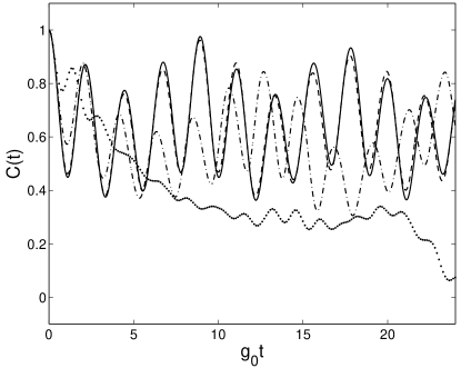
(a) $C(t)$

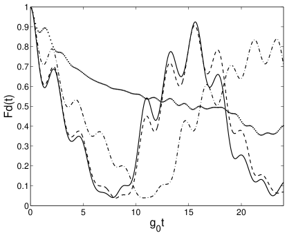
(b) $Fd1(t)$

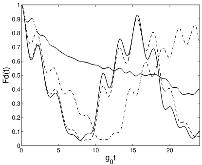
(c) $Fd2(t)$

Figure 1: Time evolution of (a) Concurrence from all $4$ Bell states, (b) Fidelity from $|e_{1,3}\rangle$, (c) Fidelity from $|e_{2,4}\rangle$ at different anisotropic parameter: $\gamma=0$ (solid curve), $\gamma=0.2$ (dashed curve), $\gamma=0.6$ (dot dashed curve), $\gamma=1.0$ (dotted curve). Other parameters are $N\rightarrow\infty$, $\mu_{0}=2g_{0}$, $g=g_{0}$, $T=g_{0}$.

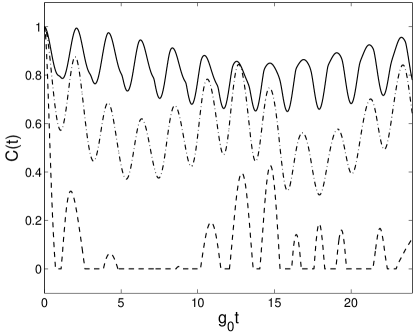
(a) $C(t)$

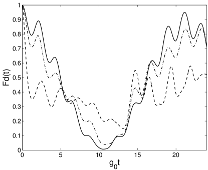
(b) $Fd1(t)$

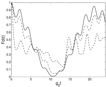
(c) $Fd2(t)$

Figure 2: Time evolution for (a) Concurrence from all $4$ Bell states, (b) Fidelity from $|e_{1,3}\rangle$, (c) Fidelity from $|e_{2,4}\rangle$ at different values of temperature: $T=0.2g_{0}$ (solid curve), $T=g_{0}$ (dot dashed curve), $T=5g_{0}$ (dashed curve). Other parameters are $N\rightarrow\infty$, $\mu_{0}=2g_{0}$, $g=g_{0}$, $\gamma=0.6$.

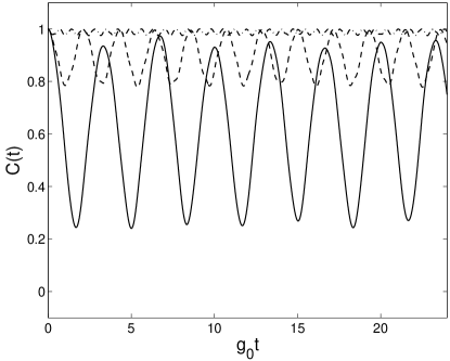
(a) $C(t)$

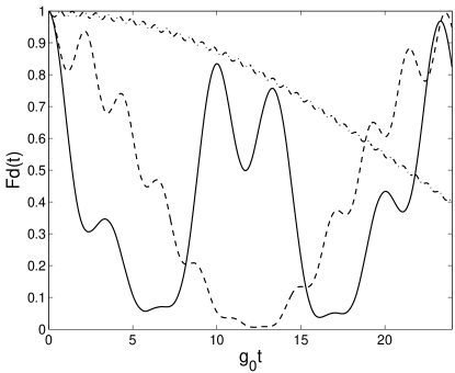
(b) $Fd1(t)$

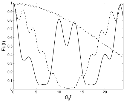
(c) $Fd2(t)$

Figure 3: Time evolution for (a) Concurrence from all $4$ Bell states, (b) Fidelity from $|e_{1,3}\rangle$, (c) Fidelity from $|e_{2,4}\rangle$ at different values of coupling strength between subsystem and bath: $g=2g_{0}$ (solid curve), $g=4g_{0}$ (dashed curve), $g=8g_{0}$ (dot dashed curve). Other parameters are $N\rightarrow\infty$, $\mu_{0}=2g_{0}$, $\gamma=0.6$, $T=g_{0}$.

The free evolution (It means the subsystem is decoupled from the bath or $g_{0}=0$.) of both concurrence and fidelity of the subsystem is time-independent, because (i) $H_{s}$ in Eq. 1 ($H_{s}=\mu_{0}(\sigma_{A}^{z}+\sigma_{B}^{z})$) can not change the entanglement degree between the two qubits; (ii) when $g_{0}=0$, the effect of the bath is excluded from the evolution of the subsystem. Thus if $g_{0}=0$, we always have $C(t)=Fd(t)=1$. In Fig. 1(a), we show different effects on the dynamics by four anisotropic parameters: $\gamma=0,0.2,0.6,1$. From the four curves, we obtain two findings. (i) When $\gamma$ is not too large, the entanglement ($C(0)=1$) can always be recovered to a high degree after some oscillations. For instances, $C(\gamma=0,g_{0}t=8.960)=0.974631$, $C(\gamma=0.2,g_{0}t=8.912)=0.961513$, $C(\gamma=0.6,g_{0}t=12.672)=0.844158$. Yet the concurrence will never reach $1$ in a long time scale. (ii) The curve of $\gamma=1$ shows a totally different behavior from the other three cases. It keeps decreasing with some little fluctuations. Then we turn to the other sub-figures. Fig. 1(c) is almost the same as Fig. 1(b). There are some obvious disagreements between Fig. 1(b) and Fig. 1(a). For example, $C(\gamma=0,g_{0}t=8.960)=0.974631$, but at the same time, $Fd1(\gamma=0,g_{0}t=8.960)=0.101803$. In other word, when the concurrence of the subsystem has been mostly retrieved, the state of that is not simultaneously back to the its initial state. Only the combination of the concurrence and the fidelity can give a complete description of the real revival of the state. It can be testified in the case of $\gamma=0$ (solid curves in the two sub-figures). When $g_{0}t=15.624$, the concurrence evolves to $C=0.875742$ and the fidelity goes back to $Fd1=0.924277$. So at that moment, $\rho_{s}(g_{0}t)$ is mainly composed by $|e_{1,3}\rangle\langle{}e_{1,3}|$.

In Fig. 2(a), Fig. 2(b) and Fig. 2(c), we plot the dynamics of the concurrence and fidelity at different temperatures. When the temperature is not too high, such as $T=0.2g_{0}$ and $T=1g_{0}$, both concurrence and fidelity represent a periodical oscillation. At some moments, they can restore to a high degree. The restoring degree of the both quantities, however, decreases as the temperature increases. Similar to Fig. 1, the revivals of the concurrence and fidelity do not take place simultaneously. When the bath is at a high temperature, such as $T=5g_{0}$, the concurrence quickly declines to zero (to see the dashed line in Fig. 2(a)) and does not go back to $C>0$ immediately. It means that when the local spin bath is adjusted to a high temperature, it makes a sudden disappearance to the entanglement of a non-localized state and it will lose the control ability to the subsystem. This is the effect that has been called “entanglement sudden death” (ESD) Yu1 ; Yu2 . In Ref. Yu2 , after the concurrence goes abruptly to zero, it arises more or less from nowhere, since there is no local effect under the action of weak noises. Our model is still an example of ESD, however, the concurrence arises after some time due to the local thermal bath.

To find out the role of the subsystem-bath coupling strength $g$, we keep the bath at a moderate temperature $T=g_{0}$. In Fig. 3(a), all the three curves show periodical behaviors and the oscillation amplitudes are strikingly damped by increasing $g$ from $2g_{0}$ to $8g_{0}$. When $g$ is up to $8g_{0}$, the fluctuation magnitude of concurrence near $C=1$ is too small to be noticed. It is like the case of $g_{0}=0$, in which the bath is decoupled from the subsystem and $C(t)=1$. It is consistent with the claims in Refs. TWmodel ; Milburn ; Jing2 that enough strong intra-coupling strength among bath spins can make the evolution of the subsystem be completely determined by the Hamiltonian of itself $H_{s}$. But the subsystem state does not receive the same protection as the subsystem entanglement degree, especially when $g=8g_{0}$. Fig. 3(b) manifests that the revival period of fidelity is much longer than that of concurrence. In fact, because Qubit $B$ is not under the influence of the bath, the bath can not make a decoherence-suppression effect on the subsystem.

III.2 finite bath spins ($N=40$)

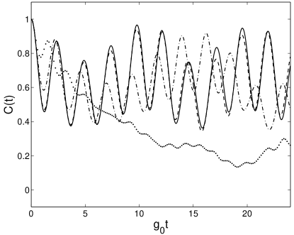
(a) $C(t)$

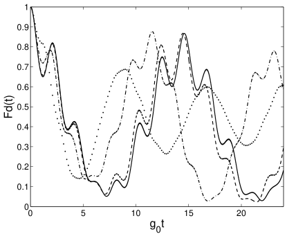
(b) $Fd1(t)$

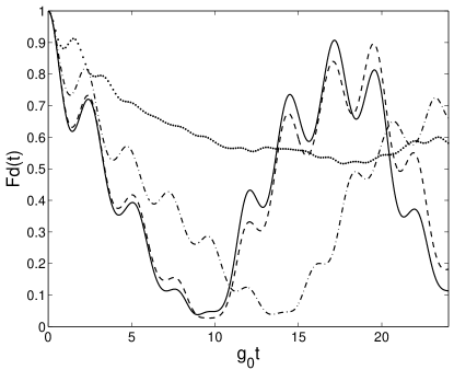
(c) $Fd2(t)$

Figure 4: Time evolution for ((a) Concurrence from all $4$ Bell states, (b) Fidelity from $|e_{1,3}\rangle$, (c) Fidelity from $|e_{2,4}\rangle$ at different values of anisotropic parameter: $\gamma=0$ (solid curve), $\gamma=0.2$ (dashed curve), $\gamma=0.6$ (dot dashed curve), $\gamma=1.0$ (dotted curve). Other parameters are $N=40$, $\mu_{0}=2g_{0}$, $g=g_{0}$, $T=g_{0}$.

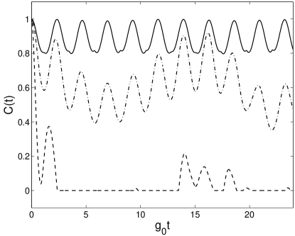
(a) $C(t)$

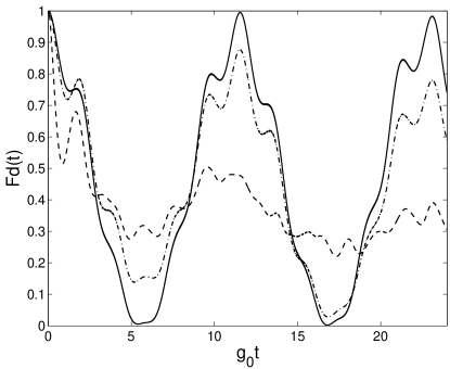
(b) $Fd1(t)$

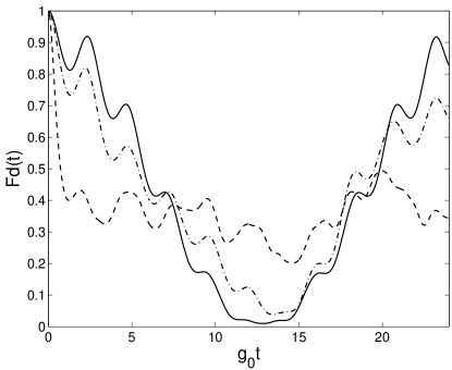
(c) $Fd2(t)$

Figure 5: Time evolution for (a) Concurrence from all $4$ Bell states, (b) Fidelity from $|e_{1,3}\rangle$, (c) Fidelity from $|e_{2,4}\rangle$ at different values of temperature: $T=0.2g_{0}$ (solid curve), $T=g_{0}$ (dot dashed curve), $T=5g_{0}$ (dashed curve). Other parameters are $N=40$, $\mu_{0}=2g_{0}$, $g=g_{0}$, $\gamma=0.6$.

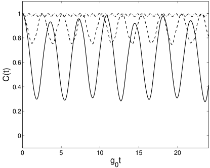
(a) $C(t)$

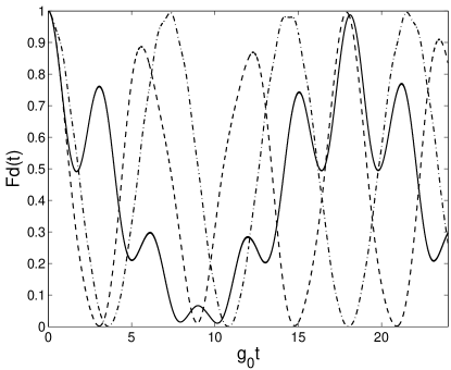
(b) $Fd1(t)$

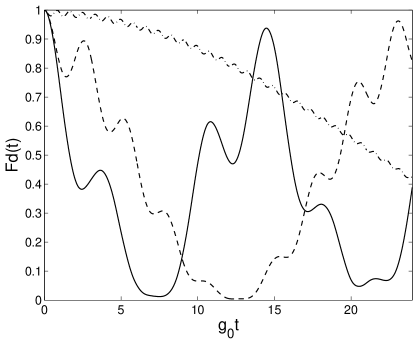
(c) $Fd2(t)$

Figure 6: Time evolution for (a) Concurrence from all $4$ Bell states, (b) Fidelity from $|e_{1,3}\rangle$, (c) Fidelity from $|e_{2,4}\rangle$ at different values of coupling strength between subsystem and bath: $g=2g_{0}$ (solid curve), $g=4g_{0}$ (dashed curve), $g=8g_{0}$ (dot dashed curve). Other parameters are $N=40$, $\mu_{0}=2g_{0}$, $\gamma=0.6$, $T=g_{0}$.

In the previous two-center-spin-spin-bath works Yuan ; Jing3 , it is supposed that the number of bath spins is infinite, which helps to reduce the Hamiltonian Eqs. 10 and 11 to a simple form. Yet as the controlling device in a real quantum information equipment, the spin bath, in principle, should be made of finite number of spins-1/2. Then in this subsection, we use the $1$st order expansion of the Hamiltonian (Eqs. 10 and 11) to introduce a finite $N$ in the present problem. The error about this approximation is about $O(1/N^{2})$ as Eq. 11 indicates. Without loss of generality, we set $N=40$ .

Comparing the result of Fig. 1 with that of Fig. 4, we can find some agreements and some disagreements. The most identical characteristic between them is that the concurrence dynamics is independent of the choice of state as long as it is one of the four Bell states. Yet when $\gamma=1$, the concurrence (dotted curve) does not decrease monotonously during the given time. For fidelity, it is shown that with a bigger anisotropic parameter $\gamma$, the curves in Fig. 4(b) oscillate with a shorter period, which is opposite to the tendency in Fig. 1(b). While Fig. 4(c) is almost the same as Fig. 1(c), with a little longer oscillation period. It seems that the fidelity evolution of the $2$nd group is not very sensitive to the bath-spin number $N$. The differences between the infinite $N$ and finite $N$ cases might arise from their different energy-level numbers and corresponding weights in our numerical scheme (in subsection III.2). Under the same requirement of numerical accuracy, for the infinite $N$, we need to consider $14,15,18$ and $20$ energy levels when $\gamma$ is $0,0.2,0.6$ and $1$ respectively; for $N=40$, we calculate $9,10,17$ and $18$ levels respectively.

In the comparison of Fig. 5 with Fig. 2, we can also find the effect of a finite $N$. At low temperature ($T=0.2g_{0}$), the entanglement degree of the subsystem qubits oscillates with a nearly perfect period between the value of $0.8$ and $1.0$ (the solid curve in Fig. 5(a)). However, the subsystem of Group $1$ (Group $2$) goes back to its own initial state only once in almost five (ten) revival periods of concurrence, which is illustrated by the corresponding curve in Fig. 5(b) (Fig. 5(c)). It is obvious that the increase of the temperature will also destroy this perfect oscillation. When $T=1g_{0}$, the second peak value, $C(g_{0}t=16.19)=0.918798$ is lower than the first one $C(g_{0}t=0)=1$ (to see the dot dashed curve in Fig. 5(a)) and the peak $Fd1(g_{0}t=11.55)=0.877301$ is higher than $Fd1(g_{0}t=23.13)=0.779953$ (to see the dot dashed curve in 5(b)). When the temperature is up to $5g_{0}$, the entanglement vanishes to zero in a fairly short stretch of time. The entanglement “death” time is longer than that in the case of $N\rightarrow\infty$ (Fig. 2). So whether $N\rightarrow\infty$ or $N$ is finite, the revival of the concurrence after ESD results from the effect of thermal bath.

For the subsystem-bath coupling $g$, the dynamics of concurrence in the case of $N=40$ (to see Fig. 6(a)) is almost the same as that in the $N\rightarrow\infty$ case (to compare it with Fig. 3(a)). The evolution of the fidelity of the $1$st group shows significant changes when $N$ is changed from infinity (Fig. 3(b)) to $40$ (Fig. 6(b)) while the fidelity of the $2$nd group does not show very obvious changes. And for the $1$st group, all the three cases behave periodical oscillations. They manifest that the subsystem in the condition of $N=40$ can be restored to the initial state with more chances or possibilities than that in the condition of $N\rightarrow\infty$.

IV Conclusion

We studied the time evolution of two separated qubit spins with a thermal equilibrium bath composed of infinite or finite spins in a quantum anisotropic Heisenberg XY model. The bath can be treated effectively as a single pseudo-spin of $N/2$ according to the symmetry of the Hamiltonian. By the Holstein-Primakoff transformation and the first order of $1/N$ expansion, it is further considered as a single-mode boson field. The pair of qubits served as an quantum information device is initially prepared in a Bell state. It is interesting that the concurrence and the fidelity dynamics of the subsystem can be controlled by some characteristic parameters of the spin bath. Through the adjustment, we show that (i) the concurrence dynamics of the subsystem is independent of the initial state, whether $N$ is infinite or finite, however, the fidelity dynamics is divided into two groups; (ii) smaller anisotropic parameter $\gamma$ can help the subsystem to evolve into a highly-entangled state, but this restoration should be measured by the combination of concurrence and fidelity; (iii) the bath at higher temperature makes a sudden death to the entanglement (ESD) of the subsystem and strongly destroys the fidelity of that; (iv) the spin-bath can help to keep the high entanglement degree between the two subsystem spins in the condition of large intra-coupling $g$.

- (1) M. A. Nielsen and I. L. Chuang, Quantum Computation and Quantum Information (Cambridge University Press, Cambridge, 2000).
- (2) C. H. Bennett, H. J. Bernstein, S. Popescu, and B. Schumacher, Phys. Rev. A 53, 2046 (1996).
- (3) R. Horodecki, P. Horodecki, M. Horodecki, and K. Horodecki, arXiv:quant-ph/0702225(2007).
- (4) R. F. Werner, Phys. Rev. A 40, 4277 (1989).
- (5) D. M. Greenberger, M. Horne, and A. Zeilinger, Bell s Theorem, Quantum Theory, and Conceptions of the Universe (Kluwer Academic Publishers, Dordrecht, 1989).
- (6) W. Dür, G. Vidal, and J. I. Cirac, Phys. Rev. A 62, 062314 (2000).
- (7) D. Loss, and D. P. DiVincenzo, Phys. Rev. A 57, 120 (1998).
- (8) B. E. Kane, Nature (London) 393, 133 (1998).
- (9) R. Tanaś and Z. Ficek, J. Opt. B, 6, 90 (2004)
- (10) T. F. Jordan, A. Shaji, and E.C.G. Sudarshan, arXiv:quant-ph/0704.0461v1(2007).
- (11) B. Schumacher, Phys. Rev. A 54, 2614(1996).
- (12) H. Barnum, M.A. Nielsen, and B. Schumacher, Phys. Rev. A 57, 4153(1998).
- (13) T. Yu and J.H. Eberly, arXiv:0707.3215v1.
- (14) H. P. Breuer and F. Petruccione, The Theory of Open Quantum Systems (Oxford University Press, Oxford, 2002).
- (15) U. Weiss, Quantum Dissipative Systems, (World Scientific, 2nd ed) (1999).
- (16) H. P. Breuer, D. Burgarth, and F. Petruccione, Phys. Rev. B 70, 045323 (2004).
- (17) X. Z. Yuan, H. J. Goan, and K. D. Zhu, Phys. Rev. B 75, 045331 (2006).
- (18) L. Tessieri and J. Wilkie, J. Phys. A 36, 12305 (2003).
- (19) Dawson C M, Hines A P, Mekenzie R H, Milburn G J, Phys. Rev. A 71, 052321, (2005)
- (20) J. Jing and H. R. Ma, Chin. Phys. 16(06), 1489 (2007).
- (21) A. O. Caldeira and A. J. Leggett, Ann. Phys., NY. 149, 374 (1983).
- (22) N. V. Prokofev and P. C. Stamp, Rep. Prog. Phys. 63, 669 (2000).
- (23) G. Burkard, D. Loss and D. P. DiVincenzo, Phys. Rev. B 59, 2070 (1999).
- (24) C. W. Gardiner, Quantum Noise, Springer-Verlag, Berlin, Heidelberg, New York (1991)
- (25) S. Shresta, C. Anastopoulos, A. Dragulescu, and B. L. Hu, arXiv:quant-ph/0408084 v1 13 Aug (2004)
- (26) S. Paganelli, F. de Pasquale, and S. M. Giampaolo, Phys. Rev. A 66, 052317 (2002).
- (27) M. Lucamarini, S. Paganelli, and S. Mancini, Phys. Rev. A 69, 062308 (2004).
- (28) A. Hutton and S. Bose, Phys. Rev. A 69, 042312 (2004).
- (29) J. Jing and Z. G. Lü, Phys. Rev. B to be published (2007).
- (30) Y. Hamdouni, M. Fannes, and F. Petruccione, Phys. Rev. B 73, 245323 (2006).
- (31) A. Einstein, B. Podolsky, and N. Rosen, Phys. Rev. 47, 777 (1935);
- (32) J. Bell, Physics 1, 195 (1964);
- (33) H. P. Breuer, Phys. Rev. A 69, 022115 (2004).
- (34) N. Canosa and R. Rossignoli, Phys. Rev. A 73, 022347 (2006).
- (35) Z. Ficek and S. Swain, Quantum Interference and Coherence: Theory and Experiments (Springer, New York, 2005).
- (36) T. Holstein and H. Primakoff, Phys. Rev. 58, 1098 (1949).
- (37) J. Jing and H. R. Ma, Phys. Rev. E 75, 016701 (2006).
- (38) G. Arfken Mathematical Methods of Physicists, New York: Academic, 3rd ed, (1985).
- (39) V. V. Dobrovitski and H. A. De Raedt, Phys. Rev. E 67, 056702 (2003).
- (40) X. G. Hu, Phys. Rev. E, 59, 2471 (1999).
- (41) S. Hill and W. K. Wootters, Phys. Rev. Lett. 78, 5022 (1997).
- (42) W. K. Wootters, Phys. Rev. Lett. 80, 2245 (1998).
- (43) L. Fedichkin and V. Privman, arXiv: cond-mat/0610756 (unpublished).
- (44) Z. Gedik, Solid State Commun. 138, 82 (2006).
- (45) T. Yu and J. H. Eberly, Opt. Commun. 264, 393 (2006).
- (46) T. Yu and J. H. Eberly, Phys. Rev. Lett. 97, 140403 (2006).