On a generalised model for time-dependent variance with long-term memory

Abstract

The ARCH process (R. F. Engle, $1982$) constitutes a paradigmatic generator of stochastic time series with time-dependent variance like it appears on a wide broad of systems besides economics in which ARCH was born. Although the ARCH process captures the so-called “volatility clustering” and the asymptotic power-law probability density distribution of the random variable, it is not capable to reproduce further statistical properties of many of these time series such as: the strong persistence of the instantaneous variance characterised by large values of the Hurst exponent ($H>0.8$), and asymptotic power-law decay of the absolute values self-correlation function. By means of considering an effective return obtained from a correlation of past returns that has a $q$-exponential form ($\exp_{q}\left[x\right]\equiv\left[1+\left(1-q\right)\,x\right]^{\frac{1}{1-q}}$, $\left(q\in\Re\right)$, and $\exp_{1}\left[x\right]=e^{x}$) we are able to fix the limitations of the original model. Moreover, this improvement can be obtained through the correct choice of a sole additional parameter, $q_{m}$. The assessment of its validity and usefulness is made by mimicking daily fluctuations of $SP500$ financial index.

The time evolution analysis of both physical and non-physical observables plays a central role in nowadays scientific research devoted to complexity. Explicitly, studies on time series with geophysical, meteorological, physiological, and financial origin, amid others, have populated scientific literature particularly during the last two decades complexity . Although each type of system has its own (microscopic) dynamical mechanism, the fact is that certain time series obtained from so dispair systems, like those mentioned above, exhibit common statistical features such as asymptotic power-law decaying probability density functions, and a long-lasting power-law-like self-correlation function of the magnitude of the time series observable, notwithstanding a fast vanishing or null self-correlation function of the variable itself. This especial class of time series has usually been associated with stochastic processes which have time-dependent variance, mathematically defined as heteroskedasticity, in contrast to the other type of time series, said homoskedastic, that present a constant value for the variance. Customarily, the profile of heteroskedastic time series is also reminiscent of on-off intermittency on-off , i.e., large values of the variable upon analysis are typically followed by other large values, but with an arbitrary sign. Within a financial context, this behaviour has been found in price fluctuations of stocks traded in financial markets or inflation econofisica . In $1982$, to further mimic the latter, R.F. Engle introduced the autoregressive conditional heteroskedasticity ($ARCH$) process engle . This process is considered as a cornerstone of econometrics fact that awarded Engle the $2003$ Nobel Memorial Prize in Economics “for methods of analysing economic time series with time-varying volatility” . Albeit its attested expressed in its broad application and generalisations arch-rev , Engle’s $ARCH$ process is unable to properly reproduce the long-lasting behaviour of the volatility self-correlation function, because it only leads to an exponential decay of this function boller . In the sequel of this manuscript we propose a generalisation of the celebrated $ARCH\left(1\right)$ process by introducing a memory kernel emerging from current non-extensive statistical mechanics formalism GM-CT . As a result, we are able to obtain the asymptotic power-law behaviour of the random variable probability density function, which is notably described by $q$-Gaussian distributions, and to mend the shortcoming of Engle’s process. The usefulness of this generalisation is shown by modelling daily fluctuations of $SP500$ financial index.

Following Engle engle , we define an autoregressive conditional heteroskedastic ($ARCH$) time series as a discrete stochastic process, $z_{t}$,

$$z_{t}=\sigma_{t}\ \omega_{t},$$ (1)

where $\omega_{t}$ is an independent and identically distributed random variable with null mean and unitary variance, i.e., $\left\langle\omega_{t}\right\rangle=0$ and $\left\langle\omega_{t}^{2}\right\rangle=1$. Henceforth we call $z_{t}$ as return. Normally, $\omega$ is associated with a Gaussian distribution (which we have used throughout this work), but other distributions for $\omega$ have been presented noise-gen . In the seminal paper of reference engle , it has been suggested a possible dynamics for $\sigma_{t}^{2}$ (hereinafter denominated as squared volatility) defining it as a linear function of past squared values of $z_{t}$,

$$\sigma_{t}^{2}=a+\sum\limits_{i=1}^{s}b_{i}\ z_{t-i}^{2},\qquad\left(a,b_{i}\geq 0\right).$$ (2)

For its linear dependence on $z_{t-i}^{2}$, eq. (1), together with eq. (2), have been coined as $ARCH\left(s\right)$ linear process. In financial practice, namely price fluctuation modelling, the case $s=1$ ($b_{1}\equiv b$) is, by far, the most studied and applied of all $ARCH$-like processes. It can be easily verified, even for all $s$, that, although $\left\langle z_{t}\ z_{t^{\prime}}\right\rangle\sim\delta_{t\,t^{\prime}}$, correlation $\left\langle\left|z_{t}\right|\ \left|z_{t^{\prime}}\right|\right\rangle$ is not proportional to $\delta_{t\,t^{\prime}}$. As a matter of fact, it has been proved for $s=1$ that, $\left\langle\left|z_{t}\right|\ \left|z_{t^{\prime}}\right|\right\rangle$ decays as an exponential law with characteristic time $\tau\equiv\left|\ln b\right|^{-1}$, which does not reproduce empirical evidences. In addition, it can be verified that, the process is stationary with a stationary variance, $\bar{\sigma}$,

$$\bar{\sigma}=\frac{a}{1-b},\qquad(b>1),$$ (3)

It has also been proved that, even for large $s$, the exponential decay of $\left\langle\left|z_{t}\right|\ \left|z_{t^{\prime}}\right|\right\rangle$ remains (check ref. boller for details). Furthermore, the introduction of a large value for parameter $s$ gives rise to implementation problems. In other words, when $s$ is large, it is very hard to find a set of $\left\{b_{i}\right\}$, since it represents the evaluation of a large number of fitting parameters . Despite instantaneous volatility fluctuation, the $ARCH(1)$ process is actually stationary and it presents a stationary returns probability density function with larger kurtosis than the distribution $P(\omega)$. The kurtosis excess is precisely the outcome of such time-dependence of $\sigma_{t}$. Correspondingly, when $b=0$, the process reduces to generating a signal with the same PDF of $\omega$, but with a standard variation $\sqrt{a}$.

We shall now introduce our variation on the $ARCH$ process. Explicitly, we consider a $ARCH\left(1\right)$ process where an effective immediate past return, $\tilde{z}_{t-1}$, is assumed in the evaluation of $\sigma_{t}^{2}$. By this we mean that we have changed eq. (2) by

$$\sigma_{t}^{2}=a+b\,\tilde{z}_{t-1}^{2},\qquad\left(a,b_{i}\geq 0\right),$$ (4)

in which the effective past return is calculated according to

$$\tilde{z}_{t}^{2}=\sum\limits_{i=t_{0}}^{t}\mathcal{K}\left(i-t\right)\,z_{i}^{2},\qquad\left(t_{0}\leq t\right),$$ (5)

where

$$\mathcal{K}\left(t^{\prime}\right)=\frac{1}{\mathcal{Z}_{q_{m}}\left(t^{\prime}\right)}\exp_{q_{m}}\left[t^{\prime}\right],\qquad\left(t^{\prime}\leq 0,q_{m}<2\right)$$ (6)

with

$$\exp_{q}\left[x\right]\equiv\left[1+\left(1-q\right)\,x\right]_{+}^{\frac{1}{1-q}},$$ (7)

$\mathcal{Z}_{q_{m}}\left(t^{\prime}\right)\equiv\sum_{i=-t^{\prime}}^{0}\exp_{q_{m}}\left[i\right]$ ($\left[x\right]_{+}=\max\left\{0,x\right\}$ ). For $q=-\infty$, we obtain the standard $ARCH\left(1\right)$, and for $q=1$, we have $\mathcal{K}\left(t^{\prime}\right)$ with an exponential form since $\exp_{1}\left[x\right]=e^{x}$ GM-CT . Although it has a non-normalisable kernel, let us refer that the value $q_{m}=\infty$ corresponds to the situation in which all past returns have the same weight, $\mathcal{K}\left(t^{\prime}\right)=1/(t-t_{0}+1).$ The introduction of an exponential kernel has already been made in dose but, as stated therein, it is not able to capture the long-lasting correlation in $\sigma_{t}$ (or $\left|z_{t}\right|$), at least for financial markets . Even though, we surmise that some systems (apart those we aim to replicate herein) might have a set of its statistical properties well-described by processes for which $q_{m}\leq 1$. Considering the process as stationary, it is not difficult to verify that eq. (3) holds.

Moving ahead on the study of our proposal we have performed numerical realisations, based on eq. (1) and eq. (4), from which we have analysed the return probability density function (PDF), the Hurst exponent feder of $\left|z_{t}\right|$ integrated signal as well as the $\left|z_{t}\right|$ self-correlation function. In order that our goal is to verify the usefulness of eq. (6) we have kept $a=\frac{1}{2}$. Our option is justified by the fact that $a$ might be eliminated if we define a new variable, $z^{\prime}\equiv z/\sqrt{a}$, for which standard deviation becomes equal to 1 (when $b=0$). Besides, expanding eq. (4),

$$\sigma_{t}=\sqrt{1+b\,\tilde{z}_{t}^{\prime\,2}}\,\sim\,1+\frac{b\,\tilde{z}_{t}^{\prime\,2}}{2}+\mathcal{O}\left(\tilde{z}_{t}^{\prime\,4}\right),$$

and considering a continuous time approach in eq. (1), we might interpret $a$ as the coefficient that is related to the magnitude of additive noise, which does not lead to “fat tails” in $p\left(z\right)$, whereas $b$ is associated with the strength of multiplicative noise which is responsible for the emergence of tails in $p\left(z\right)$  gardiner .

To mathematically describe the returns probability density function we have used the $q$-Gaussian function

$$p\left(z\right)=\mathcal{A}e_{q}^{-\mathcal{B}\,z^{2}},\qquad\left(q<3\right),$$ (8)

with $\mathcal{B}=\left[\bar{\sigma}_{q}^{2}\left(3-q\right)\right]^{-1}$, where,

$$\bar{\sigma}_{q}^{2}\equiv\int z^{2}\left[p\left(z\right)\right]^{q}dz/\int\left[p\left(z\right)\right]^{q}dz,$$

is the $q$-generalised second order moment 3ver , and $\mathcal{A}$ is the normalisation constant. For $q<5/3$, $\bar{\sigma}_{q}^{2}$ relates to the usual variance according with $\bar{\sigma}_{q}^{2}\left(3-q\right)=\bar{\sigma}^{2}\left(5-3\,q\right)$ ct-GM-CT . Distribution (8) optimises non-additive (or Tsallis) entropy, $S_{q}$ ct , and it is widely applied to describe the PDF of returns in stock market indices and other natural and artificial processes which present the properties that we aim to reproduce . In the characterisation of $p\left(z\right)$, all PDF adjustments have only involved one parameter, the index $q$, since we have normalised $z$ by the standard deviation and we have divided $p\left(z\right)$ by $p\left(0\right)=\mathcal{A}$. Nevertheless, as we shall see further on, the agreement at the peak is clear-cut.

On account of difficulties  about evaluating truthful values of the self-correlation function,

$$C_{\tau}\left(x\right)=\frac{\left\langle x\left(t\right)\,x\left(t+\tau\right)\right\rangle-\left\langle x\left(t\right)\,\right\rangle^{2}}{\left\langle x\left(t\right)\,^{2}\right\rangle-\left\langle x\left(t\right)\,\right\rangle^{2}},$$ (9)

we have opted to use the integrated $\left|z_{t}\right|$ time series Hurst exponent, $H$, obtained from the trustworthy DFA method which describes the scaling of the root-mean square, $F\left(\tau\right)$, in signals, $F\left(\tau\right)\,\sim\,\tau^{H}$ ($0<H<1$)  dfa . The results of $q$ and $H$ obtained from numerical adjustment procedures are depicted in fig. 1 as functions of $b$ and $q_{m}$.

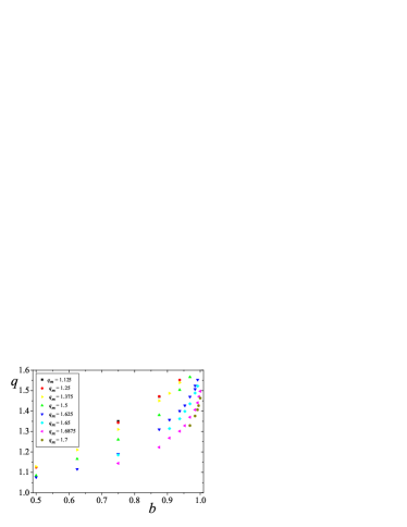
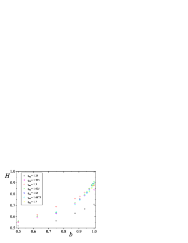
Figure 1: Left panel: Entropic index $q$ of eq. (8) versus parameter $b$ for several values of memory index $q_{m}$. All the numerical adjustments to obtain $q$ have a $\chi^{2}$ (per degree of freedom) error function of the order of $10^{-5}$ and squared correlation coefficient $R^{2}\sim 0.999$. Right panel: Hurst exponent $H$ versus parameter $b$ for several values of memory index $q_{m}$ obtained by DFA method. The numerical adjustments we have made present a correlation coefficient $R\sim 0.999$. The runs that lead to the values depicted in both panels have $10^{6}$ elements.

As it is visible from fig. 1 (left panel), for constant $q_{m}$, $q$ increases monotonically as $b$ also increases. For the same $b$ we observe that larger values of $q_{m}$ lead to smaller values of $q$. In other words, by increasing $q_{m}$, we augment memory in $\sigma_{t}^{2}$, hence volatility tends to become less fluctuating. As a consequence, $p\left(z\right)$ approaches $\omega$ distribution, since, as we have mentioned above, the time dependence of $\sigma_{t}$ is the responsible for emergence of the tails in $p\left(z\right)$. This effect is perfectly observed when $q_{m}=\infty$, for which memory efects are so strong (every single element of the past influences the present with the same weight), that after some time steps volatility remains constant.

Concerning Hurst exponent figures, we would like to refer that they have a bearing on the time interval, $\tau^{\prime}$, before the crossover into $H=\frac{1}{2}$ regime. Whatever the value of $q_{m}$ we have considered, for values of $b<0.75$, the crossover is visible with a transition $\tau$, $\tau_{c}$, which increases as $b$ gets larger. Should time series have highly persistent volatility, like price fluctuation ones, the crossover is basically unperceptive within a temporal scale up to $\tau=10^{6}$ time steps.

From the set of numerical results we have estimated the best values of $q_{m}$ and $b$ which can reproduce statistical features of a paragon of the type of time series which we have been referring to — the daily fluctuations of $SP500$ financial index econofisica . Our $SP500$ time series runs from the $3^{rd}$ January $1950$ up to the $28^{th}$ February $2007$ in a total of $14380$ business days. The daily return $z_{t}$ is computed as

$$z_{t}\equiv\ln\,S_{t}-\ln\,S_{t-1},$$

where $S_{t}$ represents the $SP500$ value at time $t$. As it is usual we have didived $z$ by its standard deviation. Gathering together the values of $q$ and $H$ for $SP500$, respectively $1.47\pm 0.02$ and $0.88$, we have verified that $q_{m}=1.6875$ and $b=0.99635$ are able to reproduce, with a remarkable agreement, both the return probability density function and the Hurst exponent as it is exhibited on fig. 2 and fig. 3. Further, when we have compared, a posteriori, the self-correlation functions of $\left|z_{t}\right|$, eq. (9), we have verified the same qualitative behaviour. In fact, despite both of the short range available for fitting and the fluctuations, a quite similar power-law decay with an exponent of $0.73\pm 0.01$ for our model and $0.71\pm 0.02$ for $SP500$ as shown on fig. 4. Specifically, and according to fig. 4, the two curves stand basically side by side for $\tau>20$ in a $\log-\log$ scale.

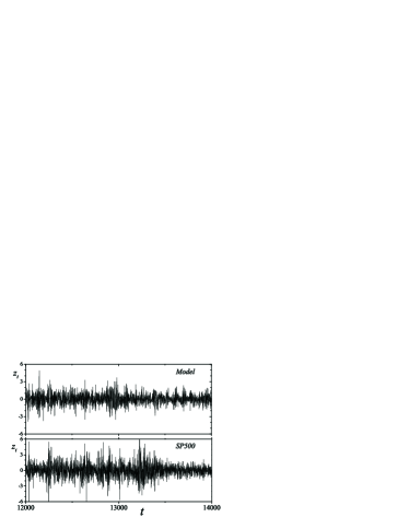
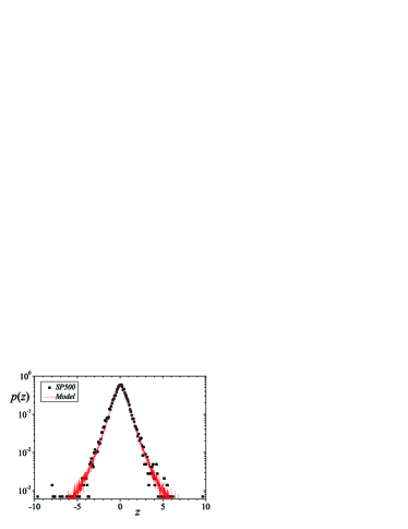
Figure 2: Left panels: Excerpts of $SP500$ daily normalised return times series with $2000$ elements, from the $10^{th}$ September $1997$ to the $25^{th}$ October $2005$, and model (with $q_{m}=1.6875$ and $b=0.99635$) for mere illustration proposes. Right panel: Probability density function $p\left(z\right)$ versus (normalised) $z$, obtained from the whole time series shown on left panels, in $\log$-linear scale (symbols are used for $SP500$ PDF and line for model PDF). As it can be seen the accordance is quite good. For $SP500$ ftting $q=1.47\pm 0.2$ ($\chi^{2}=6\times 10^{-5}$ and $R^{2}=0.99$). In both cases $z$ is expressed in standard deviation units.

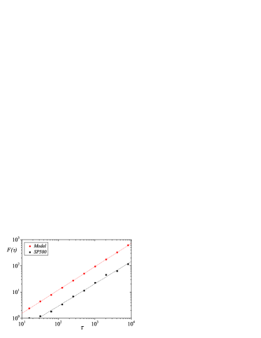
Figure 3: Root-mean square fluctuations, $F\left(\tau\right)$, versus $\tau$ of the time series of fig. 2. The values obtained from numerical fitting are $H=0.883\pm 0.005$ for $SP500$ (squares) and $H=0.886\pm 0.003$ for the model (circles).

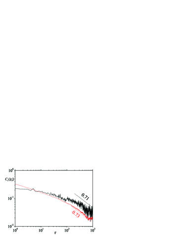
Figure 4: Absolute returns self-correlation function $C_{\tau}\left(\left|z_{t}\right|\right)$ versus $\tau$ in $\log$-$\log$ scale. The similarity on the qualitative behaviour of the two curves is evident. Although the fluctuation, evaluating the decay exponents as a result of a fitting procedure for large $\tau$ we have obtained $0.73\pm 0.01$ for the model and $0.71\pm 0.03$ for $SP500$.

To summarise, in this manuscript we have introduced a generalisation of Engle’s proposal for generating instantaneous volatility in heteroskedastic processes. This modification refers to the introduction of a memory kernel which has an asymptotic power-law dependence defined by a parameter $q_{m}$. Apart from the fact that our alteration has been able to reobtain the non-Gaussian PDF for the random variable, $z_{t}$, it has also been successful about reproducing the long-lasting (asymptotic power-law decaying) self-correlation of the magnitude of $z_{t}$ exhibited by a large number of phenomena. The improvement in the reproduction of statistical features of such a kind of time series has been achieved by considering just one additional parameter, $q_{m}$, which represents a clear simplification against $ARCH\left(s\right)$ (with $s\gg 1$), that only manage to exhibit a exponential volatility self-correlation function with large characteristic time, or other heteroskedastic processes arch-rev . By exhaustive numerical analysis of our model we have found a pair of values, $q_{m}$ and $b$, with which we have mimicked daily fluctuations of $SP500$. The resemblance between $SP500$ time series and the signal obtained by numerical application of our suggestion is remarkably good for the probability density function and the Hurst exponent. In a qualitative sense, the correlation function has also been quite well described. The quantitative discrepancies verified in $C_{\tau}\left(\left|z_{t}\right|\right)$ and $F\left(\tau\right)$ might be solved if we modify kernel (6) by introducing a sort of “characteristic time”, $T$,i.e., in eq. (6) $t^{\prime}\rightarrow t^{\prime}/T$, as another parameter.

It is well known that there are an infinity of dynamics whose outcome is the same probability density function. However, as far as we are able to obtain an appropriate reproduction of further statistical properties, as it is the case we have just presented, we will be approaching our models towards the nature of the system upon study. This is certainly important when the models are applied, e.g., on forecasting purposes. It is on this basis we support the relevance of our propose.

In respect of financial markets, and considering a macroscopic approach, our model permit us to say that price fluctuations are actually dependent on their history, but on a asymptotically scale-free way tsallis-ca , as it is exhibited by the majority of the so-called complex systems. Such a dependence is in contrast with the usual, and analitycally simpler, exponential treatment. On a practical way, this also means that past events take long time to loose their importance.

Last of all, owing to $C_{\tau}\left(\left|z_{t}\right|\right)$ asymptotic power-law decay, as it is visible from eq. (7), we could make a correspondence between the decay exponents and a correlation index, $q_{c}$. By this we get $q_{c}=2.37\pm 0.03$ for our model and $q_{c}=2.41\pm 0.06$ for $SP500$. Such an association introduces an alternative triplet of entropic indices tsallis-villa , namely $\left\{q_{m},q,q_{c}\right\}$, related to non-extensive statistical mechanics formalism that could characterise this type of systems.

SMDQ acknowledges C. Tsallis for his continuous encouragement and discussions as well as E. M. F. Curado for helpful and stimulating conversations at early and final stages of the work. E. P. Borges and F. D. Nobre are thanked for comments made on previous versions of this manuscript. This work has benefited from infrastructural support from PRONEX/MCT (Brazilian agency) and financial support from FCT/MCES (Portuguese agency).

References

- (1) Skjeltorp A. T., and Vicsek T. (editors), Complexity from Microscopic to Macroscopic Scales: Coherence and Large Deviations (Kluwer Academic Publishers, Dordrecht, 2002); Beck C., Benedek G., Rapisarda A., and Tsallis C. (editors), Complexity, Metastability And Nonextensivity (World Scientific, Singapore, 2005).
- (2) Platt N., Spiegel E. A., and Tresser C., Phys. Rev. Lett. 70 (1993) 279.
- (3) Bouchaud J. P., and Potters M., Theory of Financial Risks: From Statistical Physics to Risk Management, (Cambridge University Press, Cambridge, 2000). Mantegna R. N., and Stanley H. E., An Introduction to Econophysics: Correlations and Complexity in Finance, (Cambridge University Press, Cambridge, 1999).
- (4) Engle R. F., Econometrica 50 (1982) 987.
- (5) Engle R. F., and Patton A. J., Quantitatit. Finance 1 (2001) 237; Andersen T. G., Bollerslev T., Christofferssen P. F., and Diebold F. X., Volatility forecasting, PIER 05-11 working paper, 2005.
- (6) Bollerslev T., Chou R. Y., and Kroner K. F., J. Econometrics 52 (1992) 5; Engle R. F., and Gallo G. M., J. Econometrics 3 (2006) 131.
- (7) Gell-Mann M., and Tsallis C. (editors), Nonextensive Entropy - Interdisciplinary Applications (Oxford University Press, New York, 2004).
- (8) Pobodnik B., Ivanov P. Ch., Lee Y., Cheesa A., and Stanley H. E., Europhys. Lett. 50 (2000) 711; Duarte Queirós S. M., and Tsallis C., Europhys. Lett. 69 (2005) 893.
- (9) Poon S. H., and Granger C. W. J., J. Econ. Lit. 41 (2003) 478.
- (10) Dose C., Porto M. , and Roman H. E., Phys. Rev E 67 (2003) 067103.
- (11) Borland L., arXiv:cond-mat/0412526 (preprint, 2004)
- (12) Feder J., Fractals (Plenum Press, New York, 1988).
- (13) Gardiner C. W., Handbook of Stochastic Methods for Physics, Chemistry and the Natural Sciences (Springer-Verlag, Berlin, 2004).
- (14) Tsallis C., Mendes R. S., and Plastino A. R., Physica A 261 (1998) 534.
- (15) Gell-Mann M., and Tsallis C., Nonextensive Entropy - Interdisciplinary Applications (Oxford University Press, New York, 2004).
- (16) Tsallis C., J. Stat. Phys. 52 (1988) 479. A regularly updated bibliography on the subject is avaible at http://tsallis.cat.cbpf.br/biblio.htm; Curado E. M. F., and Tsallis C., J. Phys. A 24 (1991) L69; 24 (1991) 3187; 25 (1992) 1019; Prato D., and Tsallis C., Phys. Rev. E 60 (1999) 2398.
- (17) Peng C.-K., Buldyrev S. V., Havlin S., Simons M., Stanley H. E., and Goldberger A. L., Phys. Rev. E 49 (1994) 1685.
- (18) Rohlf T., and Tsallis C., Physica A 379 (2007) 465.
- (19) Tsallis C., Physica A 340 (2004) 1.