Monitoring the Violent Activity from the Inner Accretion Disk of the Seyfert 1.9 Galaxy NGC 2992 with RXTE

Abstract

We present the results of a one year monitoring campaign of the Seyfert 1.9 galaxy NGC 2992 with RXTE. Historically, the source has been shown to vary dramatically in 2–10 keV flux over timescales of years and was thought to be slowly transitioning between periods of quiescence and active accretion. Our results show that in one year the source continuum flux covered almost the entire historical range, making it unlikely that the low-luminosity states correspond to the accretion mechanism switching off. During flaring episodes we found that a highly redshifted Fe K line appears, implying that the violent activity is occurring in the inner accretion disk, within $\sim 100$ gravitational radii of the central black hole. We also found that the spectral index of the X-ray continuum remained approximately constant during the large amplitude variability. These observations make NGC 2992 well-suited for future multi-waveband monitoring, as a test-bed for constraining accretion models.

1 INTRODUCTION

NGC 2992 is a relatively nearby ($z=0.00771$) Seyfert 1.9 galaxy. Observations of NGC 2992 have been made by every X-ray mission since its discovery by $HEAO-1$ in 1977 (Piccinotti et al. 1982). Fig. 1 shows the historical light curve (2–10 keV flux) for X-ray observations over the past $\sim 30$ years (Piccinotti et al. 1982, Mushotzky 1982, Turner & Pounds 1989, Turner et al. 1991, Nandra & Pounds 1994, Weaver et al. 1996, Gilli et al. 2000, Yaqoob et al. 2007). In 1994, ASCA observed NGC 2992 to have a very low X-ray continuum flux compared with previous observations (Weaver et al. 1996), down by a factor of $\sim 20$ since it was first detected. The ASCA data revealed a very prominent, narrow Fe K$\alpha$ emission line, believed to have originated in matter distant from the supermassive black hole (possibly in the putative obscuring torus). Later, X-ray observations with BeppoSAX (Gilli et al. 2000) showed a revival to a high-flux state. This was accompanied by complex variability in the Fe K$\alpha$ line profile, which appeared to have possible contributions from radiation originating in both the accretion disk and distant matter. Gilli et al. (2000) suggested that the variation in continuum flux was evidence of quenching and revival of accretion on a timescale of years. In fact, they believed that BeppoSAX witnessed a revival of the AGN between its two observations, which were separated by about a year in the period 1997–1998. Not shown in Fig. 1 is a third observation made by BeppoSAX during its last week of operation in April 2002, from which only PDS data were taken (see Beckmann et al. 2007). Hard X-ray data taken by INTEGRAL (in 2005 May) and Swift (in 2005–2006) are also presented by Beckmann et al. (2007).

We obtained observing time for a one-year monitoring campaign of NGC 2992 with the Rossi X-ray Timing Explorer (RXTE) beginning in 2005. NGC 2992 had never been observed with RXTE prior to this campaign. The goal was to test the response of the Fe K$\alpha$ line to the variation in the X-ray continuum. Spectral analysis of these data revealed an unexpected result: the variation in flux for the twenty-four RXTE observations covered nearly the entire dynamical range in flux in the historical data in less than a year. Previously it was thought that the variation occurred over decades, but the RXTE data showed flares in the X-ray continuum flux on timescales of days. Additionally, the Fe K$\alpha$ emission line (that is present in the majority of the observations and centered at $\sim 6.4$ keV in most cases) was redshifted and broadened during high-flux periods, implying that we may have been witnessing short-term flaring activity (on the order of days to weeks) from the inner regions of the accretion disk.

In §2, we describe the RXTE data and our data reduction process. We describe the results of our spectral analysis of the data in §3, including a discussion of the variability of the Fe K$\alpha$ emission line and the physical implications. In §4 we summarize the conclusions of our analysis. An Appendix is included to discuss a calibration feature found in the data in the 8–9 keV range.

2 OBSERVATIONS & DATA REDUCTION

NGC 2992 was observed between 2005 March 4 and 2006 January 28 with the RXTE Proportional Counter Array (PCA; Jahoda et al. 2006). We obtained data from a total of twenty-four observations. The observation log is given in Table 1; hereafter we will refer to each observation as obs 1 to 24 as listed in Table 1. It can be seen that the interval between observations ranged from $\sim 3$ to 33 days.

The PCA is an array of five Proportional Counter Units (PCUs), each with a net geometric collecting area of $\sim 1600$ cm² (Jahoda et al. 2006). Each PCU consists of 3 layers of a mixture of Xenon (90%) and Methane (10%) gas and a $1^{\circ}$ collimator (FWHM). For energies less than 10 keV, $\sim$ 90% of the cosmic photons and 50% of the internal instrumental background are detected in the top layer (layer 1) of the Xenon/Methane detector. Therefore, in order to maximize the signal-to-noise ratio, only data from layer 1 of the PCUs were used.

Fewer of the PCUs were in operation later in the mission, so we did not obtain data from all five units. For two observations (obs 2 and obs 3), PCUs 0, 1, and 2 were operational; however, only PCU 0 and PCU 2 were operational for all twenty-four of the NGC 2992 observations. In order to perform a uniform analysis of all of the observations, we discarded the PCU 1 data for obs 2 and obs 3, and only used data from PCU 0 and PCU 2.

In the spring of 2000 (May 12), the propane layer in PCU 0 lost pressure and thus the calibration and background subtraction model were adversely affected (Jahoda et al. 2006). Since then, the calibration and background estimation have improved, so we retained the PCU 0 data, but performed initial analyses on PCU 0 and PCU 2 separately, in order to check for inconsistencies in the two detectors. We found the variation in the results from spectral fits to the data from the two detectors to be statistically insignificant. As we will describe in §3, we analyzed the spectra from the combined PCU 0 plus PCU 2 data in addition to the individual PCU data in order to obtain better statistics on the important model parameters.

The data were selected to exclude time intervals when the Earth’s elevation angle was less than $10^{\circ}$, during passage of the satellite through the South Atlantic Anomaly (SAA), and during times of high electron contamination (ie, the housekeeping parameter ‘ELECTRON2’ was selected to be greater than 0.1). The background was estimated with the program PCABACKEST, using the mission-long ‘Faint’ model file pca_bkgd_cmfaintl7_eMv20031123.mdl (Jahoda et al. 2006). Spectral response matrices were made for each of the observations for both PCU 0 and PCU 2 using pcarmf version 10.1 and the channel-to-energy calibration file pca_e2c_e05v03.fits.

We extracted spectra and light curves for PCU 0 and PCU 2 for each of the twenty-four observations. In addition, we co-added the PCU 0 and PCU 2 data to make twenty-four combined (PCU 0 + PCU 2) spectra. In obs 7 and obs 15, we found flares in the PCU 0 light curves, so we applied further data selection with time cuts to remove those periods from the PCU 0 data. These selection criteria resulted in net exposure times for the PCU 0 + PCU 2 data in the range of $\sim 1.5$ to $\sim 6.5$ ks, as shown in Table 1. The grand total integration time for the twenty-four observations, summed over PCU 0 + PCU 2, was 133.088 ks. The mean, full-band, background-subtracted count rates for the combined PCU 0 + PCU 2 data varied by over an order of magnitude, ranging from $\sim 0.8$ to $\sim 10.6$ cts/s (see Table 1).

3 SPECTRAL FITTING RESULTS

We modeled the PCA spectra using XSPEC version 11.3.2 (Arnaud 1996). Preliminary examination of the spectra revealed poor background subtraction above $\sim 15$ keV. Since the PCA data below $\sim 3$ keV are not well calibrated (Jahoda et al. 2006), we performed spectral fitting in the 3–15 keV range. We used $\chi^{2}$ as the fit statistic. In all of the model fitting the Galactic column was fixed density at $N_{\rm H}=5.26\times 10^{20}\rm\ cm^{-2}$ (Dickey & Lockman 1990). Although the 3–15 keV energy range is not sensitive to Galactic absorption, we included it for consistency with models in the literature that were fitted to lower energy data. All model parameters will be referred to in the source frame.

3.1 Individual Observation Fits

We fitted a simple power-law model to each of the spectra for the twenty-four observations, initially for the PCU 0 and PCU 2 data separately and subsequently for the combined PCU data. This model consisted of two free parameters, namely the photon index ($\Gamma$) and the power-law normalization. We found, in most cases, that the plots of the data/model ratios of the twenty-four combined PCU spectra showed residuals that may correspond to the Fe K$\alpha$ emission line known to be present in the source (e.g. Weaver et al. 1996, Gilli et al. 2000). Each case was confirmed by examining the separate PCU 0 and PCU 2 fits.

We therefore proceeded to fit a power-law plus a Gaussian emission-line component to the three sets of twenty-four spectra. The model consisted of five free parameters: the power-law normalization, $\Gamma$, the centroid energy of the line ($E_{\rm Fe\ K\alpha}$) in keV, the intrinsic line width ($\sigma_{\rm Fe\ K\alpha}$) in keV, and the intensity of the line ($I_{\rm Fe\ K\alpha}$) in $\rm photons\ cm^{-2}\ s^{-1}$. Although for eight of the twenty-four fits the probability of obtaining values of $\chi^{2}$ as high as those measured from the data by chance was less than 10%, we note that our data do not include compensation for systematic errors so the goodness of fits cannot be assessed by consideration of the values of $\chi^{2}$ alone. We will return to this question when discussing fits to grouped data sets (§3.4). In cases where the line energy could not be constrained, the fit was repeated with the Fe K$\alpha$ energy fixed at the neutral Fe value of 6.4 keV. In obs 22–24, where the width of the line could not be constrained (the line was too weak), we fixed the intrinsic Gaussian line width at $\sigma_{\rm Fe\ K\alpha}$ = 0.05 keV in order to obtain statistical errors on the line intensity. This width is much less than the PCA energy resolution ($\Delta E\sim 1.02$ keV FWHM at 6 keV, Jahoda et al. 2006). For seventeen of the twenty-one remaining data sets, the decrease in $\chi^{2}$ ranged from 6.3 to 22.2 for the addition of three free parameters for the line, compared to the continuum-only fits. This corresponds to detections of the line at a confidence level greater than 90% ($\Delta\chi^{2}=6.251$ for three parameters). Three of the remaining four observations (obs 2, 11, and 12) had detections of the line at greater than 68% confidence ($\Delta\chi^{2}=3.506$ for three parameters) and one (obs 15) had a detection at only marginally less than 68% confidence ($\Delta\chi^{2}=3.4$).

We compared the values of $\Gamma$, $E_{\rm Fe\ K\alpha}$, $\sigma_{\rm Fe\ K\alpha}$, and $I_{\rm Fe\ K\alpha}$ that were obtained from spectral fits to the PCU 0 data with those obtained from the PCU 2 data and found no evidence of systematic differences. For example, Fig. 2a and Fig. 2b show plots of $\Gamma$(PCU 0) vs. $\Gamma$(PCU 2) and $I_{\rm Fe\ K\alpha}$ (PCU 0) vs. $I_{\rm Fe\ K\alpha}$ (PCU 2) respectively. Also, the ratios of the data to the model for PCU 0 and PCU 2 showed no systematic anomalies within the statistical errors. Therefore, hereafter we refer only to the results obtained from the combined PCU 0 + PCU 2 spectral fits.

The power-law plus Gaussian fit results for the combined PCU data are shown in Table 2. Statistical errors for each parameter in Table 2 are 68% confidence for $n$ interesting parameters, where $n$ = 2 or 3 (corresponding to $\Delta\chi^{2}$ = 2.279 and 3.506 respectively), depending on the number of parameters that were fixed in order to obtain stable fits during the error analysis. The power-law normalization is not included as an interesting parameter. Quoting the 68% confidence ($1\sigma$) errors facilitates statistical analysis of the results. We also quote (in brackets, below the best-fit values) 90% confidence ranges for one interesting parameter ($\Delta\chi^{2}$ = 2.706), for comparison with other results in the literature. Parameters that were fixed are labeled with ‘$f$’ in Table 2.

For twenty-one of the data sets, statistical errors were found for $\sigma_{\rm Fe\ K\alpha}$ by fixing the line energy at the best-fit value and statistical errors were found for $E_{\rm Fe\ K\alpha}$, $I_{\rm Fe\ K\alpha}$, and $\Gamma$ by fixing the line width at the best-fit value. Therefore, for these cases, 68% confidence errors were found using $\Delta\chi^{2}=3.506$ ($n=3$) for all interesting parameters. The fits became highly unstable if we allowed both $\sigma_{\rm Fe\ K\alpha}$ and $E_{\rm Fe\ K\alpha}$ to be free during the error analysis. A stable fit for the line was not obtained for obs 22, 23, and 24 since the line was not detected with sufficient statistical significance in these observations. In these cases, it was necessary to fix both the line energy at 6.4 keV and the line width at 0.05 keV to obtain statistical errors ($n=2$) for the remaining free parameters ($I_{\rm Fe\ K\alpha}$ and $\Gamma$).

3.2 Light Curve

In order to facilitate comparison with the literature, we calculated the 2–10 keV continuum flux and luminosity values by extrapolating the 3–15 keV models down to 2 keV. The 2–10 keV fluxes and luminosities are presented in Table 2. All fluxes are observed-frame values, not corrected for absorption. All luminosities are rest-frame values, corrected for absorption.

The $\sim 1$ year light curve (Fig. 3 ) ranges from $\sim 0.8\times 10^{-11}\rm\ to\sim 8.9\times 10^{-11}\ ergs\ cm^{-2}\ s^{-1}$ in 2–10 keV flux. The 2–10 keV luminosity ranges from $0.11\times 10^{43}$ to $\sim 1.17\times 10^{43}$ ergs $\rm s^{-1}$ (assuming $H_{o}=70$ km s^-1 Mpc^-1, $\Lambda=0.73$, $\Omega=1$), while the fraction of the Eddington luminosity ($L/L_{\rm edd}$) ranges from $\sim 1.5\times 10^{-3}$ to $\sim 1.8\times 10^{-2}$, assuming a black hole mass of $5.2\times 10^{7}M_{\odot}$ (Woo & Urry 2002). Historically, $L/L_{\rm edd}$ has ranged from $\sim 0.8\times 10^{-3}$ to $\sim 1.9\times 10^{-2}$. The first RXTE observation, which had the highest flux, was followed by two additional high-flux peaks (obs 4 and obs 8). The flux then dropped to $\sim 1\times 10^{-11}\rm\ ergs\ cm^{-2}\ s^{-1}$ during obs 9 to obs 12. This was followed by a slight rise in flux for obs 13 and obs 14. The flux measurements in the remaining observations stayed in the $1-2\times 10^{-11}\ \rm ergs\ cm^{-2}\ s^{-1}$ range, with the last three appearing to make an upward turn.

We quantified the variability in the RXTE light curve by calculating the fractional variability amplitude, $F_{\rm var}$, comparing this measure of variability with results obtained from RXTE monitoring of other AGN (e.g. see Vaughan et al. 2003; Markowitz et al. 2003; Markowitz & Edelson 2004). The quantity $F_{\rm var}$ is simply the square root of the excess variance, that is also used to characterize AGN variability, taking into account Poisson noise (e.g. see Turner et al. 1999). Markowitz & Edelson (2004) calculated $F_{\rm var}$ uniformly for a sample of AGN, based on 2–12 keV RXTE PCA count rates, and several monitoring durations, one of which was 216 days. Using the same energy band for NGC 2992, we obtained $F_{\rm var}=(91.5\pm 0.5)\%,(84.0\pm 0.5)\%$, and $(41.6\pm 0.8)\%$ for all 24 observations, the first 16 observations (207 days duration), and the last 14 observations (211 days duration), respectively. Our observations of NGC 2992 were spaced roughly two weeks apart except for two pairs of observations for which each pair had a separation of only three days. The count rates from these pairs of observations were averaged in order to obtain roughly equal spacing in time intervals before calculating $F_{\rm var}$. Markowitz & Edelson (2004) found that the majority of the AGN in their sample had 216-day values of $F_{\rm var}$ lying the range $\sim(1-40)\%$, and the two sources with the highest values of $F_{\rm var}$ of $\sim 60\%$ were NGC 3227 and NGC 4051 (both of these have X-ray luminosities that are similar to the luminosity of NGC 2992). Thus the high value of $F_{\rm var}$ obtained for the first part of the RXTE NGC 2992 campaign (and indeed for the whole campaign) is exceptionally high. Moreover, the value of $F_{\rm var}$ obtained for the second part of the campaign (in which NGC 2992 was much “quieter”) is still at the high end of the range that was obtained by Markowitz & Edelson (2004) for their sample of AGN.

We can compare the timescales probed by our RXTE campaign with the expected break frequency, $\nu_{b}$, given the black-hole mass, based on a correlation observed from studying samples of Seyfert galaxies and other black-hole systems (e.g. Papadakis 2004 finds $\nu_{b}\sim 15/[M_{\rm BH}/M_{\odot}]$ Hz; see also McHardy et al. 2007 and references therein). This break frequency marks the division where the power spectrum flattens from $\sim\nu^{-2}$ to $\sim\nu^{-1}$ towards lower frequencies. For NGC 2992 the predicted timescale corresponding to the break frequency is $\sim 40$ days. On the other hand, if we use the relation between the break timescale and luminosity that McHardy et al. (2007) empirically from studying a sample of AGN, we obatined $\sim 1-2$ days. Clearly, more frequent sampling than that achieved in our monitoring of NGC 2992 is required in order to derive reliable, direct, quantitative constraints on the power-spectrum amplitude and break frequency (or timescale).

3.3 Continuum & Fe K Emission Line

The photon index, $\Gamma$, ranged from $\sim 1.61\rm\ to\sim 2.25$. A plot of $\Gamma$ versus 2–10 keV flux is given in Fig. 4. It is interesting to note that, despite the significant variation in flux, $\Gamma$ is consistent with a constant value within the statistical errors. The weighted average of $\Gamma$ is $1.732\pm 0.022$. This behavior constrasts with some other Seyfert galaxies in which $\Gamma$ increases with continuum luminosity. Utilizing the 68% confidence statistical errors, we show in Fig. 5 the best-fit line energies plotted against the 2–10 keV luminosity from each observation, except for the observations in which $E_{\rm Fe\ K\alpha}$ had to be fixed (represented by open circles on the plot). With the exception of observations that were made when NGC 2992 was in a high-flux state, the line energies are consistent with 6.4 keV, confirming the presence of an Fe K$\alpha$ emission line from cool matter in the source. In the high-flux spectra, the centroid energy of the line was found to be $\sim 5.6$ keV. As will be discussed later, this may correspond to a broad component in the Fe K$\alpha$ line complex due to redshifted emission resulting from enhanced illumination of the line-emitting material in close proximity to the central black hole.

The line width, $\sigma_{\rm Fe\ K\alpha}$, was a free parameter in twenty-one of the twenty-four combined PCU 0 plus PCU 2 fits. For these observations, the best-fit value for $\sigma_{\rm Fe\ K\alpha}$ ranged from 0.0 to 1.1 keV, often with large statistical errors. A plot of Fe K$\alpha$ line intensity ($I_{\rm Fe\ K\alpha}$ ) vs. 2–10 keV luminosity is given in Fig. 6. Although the 2–10 keV luminosity varies by a factor of $\sim 11$, we see from Fig. 6 that the line intensity variability amplitude appears to be less than that of the continuum. While the 68% confidence errors of the line intensity covered a range of $0.0\ \rm to\ 46.2\times 10^{-5}\ \rm photons\ cm^{-2}\ s^{-1}$, the weighted mean of $I_{\rm Fe\ K\alpha}$ was $\sim 6.6\pm 1.0\times 10^{-5}\ \rm photons\ cm^{-2}\ s^{-1}$. The results imply a constant line intensity or significant time delays between the response of the line emission to continuum variations. For comparison of the emission line and continuum variability, we show in Fig. 7 the results of $L/L_{\rm Eedd}$, $\Gamma$, $E_{\rm Fe\ K\alpha}$, $I_{\rm Fe\ K\alpha}$ for the twenty-four observations versus time. As shown in Fig. 8, there is no clear trend in the variation of the Fe K$\alpha$ line EW with 2–10 keV continuum luminosity. Although there is larger variation at lower luminosities, the uncertainty is also greater. At higher luminosities, the EW appears to tend towards values less than 500 eV.

We can compare our measured values of the Fe K$\alpha$ line intensity with the theoretical expectation in the limit of a Thomson-thin spherically-symmetric distribution of gas surrounding a central X-ray source. In the limit of low redshift, the theoretical value of $I_{\rm Fe\ K\alpha}$ is

$$I_{\rm Fe~{}K\alpha} = 7.44\times 10^{-5}\ h_{70}^{2}\left(\frac{L_{2-10}}{10^{43}\ \rm ergs\ s^{-1}}\right)\left(\frac{<L>}{L}\right)\left(\frac{N_{\rm H}}{10^{23}\ \rm cm^{-2}}\right)\left(\frac{\Delta\Omega}{4\pi}\right)\left(\frac{\omega_{\rm K}}{0.34}\right)\left(\frac{A_{\rm Fe}}{4.68\times 10^{-5}}\right)$$ (1)

$$\left(\frac{3.4}{\Gamma+1.646}\right)(7.11^{1.7-\Gamma})\left(\frac{2-\Gamma}{0.3}\right)\left(\frac{0.764}{10^{2-\Gamma}-2^{2-\Gamma}}\right)\left(\frac{z}{0.00771}\right)^{-2}\rm photons\ cm^{-2}\ s^{-1}\hskip 42.67912pt$$

(see for example Yaqoob et al. 2001), where $L_{2-10}$ is the 2–10 keV luminosity and $(\Delta\Omega/4\pi)$ is the fraction of the sky covered by the line-emitting region, as seen by the source. Here $L$ is the measured luminosity and $<L>$ is representative of the historically averaged luminosity on timescales greater than the light-crossing time of the line-emitting region. The factor $h_{70}$ is defined as $\left(\frac{H_{0}}{70\ \rm km\ s^{-1}\ Mpc^{-1}}\right)$, where $H_{0}$ is the Hubble constant. $N_{\rm H}$ is the column density of the shell. The value of $A_{\rm Fe}$ is the iron abundance in the emitting material (relative to hydrogen) and $\omega_{\rm K}$ is the fluorescence yield. All of the factors in parentheses involving the photon index in equation 1 evaluate to $\sim 1$ for $\Gamma=1.7$, the approximate mean value found for NGC 2992 from the RXTE observations. Note that equation (1) does not represent any assumptions about NGC 2992. It is simply a theoretical limit with which results from NGC 2992 can be compared. From this comparison one can deduce constraints on the physical parameters that must apply to NGC 2992.

Overlaid on Fig. 6 are four theoretical $I_{\rm Fe\ K\alpha}$ versus luminosity curves corresponding to values of $\left(\frac{<L>}{L}\right)\left(\frac{N_{\rm H}}{10^{23}\ \rm cm^{-2}}\right)$ equal to $0.1,\ 1,\ 5$ and $10$. The curves were calculated using equation 1 with $\frac{\Delta\Omega}{4\pi}=1$ and $\Gamma=1.732$, the weighted mean value of the photon index. We took $A_{\rm Fe}$ to be $4.68\times 10^{-5}$, the solar value given in Anders & Grevesse (1989), and we used the value $\omega_{\rm K}=0.34$ as given in, for example, Palmeri et al. (2003). The typical line-of-sight $N_{\rm H}$ that has been measured by Suzaku and other missions is $\sim 10^{22}\ \rm cm^{-2}$. For this value, $\frac{<L>}{L}=1$ corresponds to the shallowest theoretical line shown on Fig. 6 (labeled with ‘0.1’), which is not a good representation of these data. Better agreement is given by a larger value of $\left(\frac{<L>}{L}\right)\left(\frac{N_{\rm H}}{10^{23}\ \rm cm^{-2}}\right)$, implying that the line-of-sight $N_{\rm H}$ is not representative of the entire system and/or the observed variation in the line intensity is affected by time delays following continuum variations. Values of $\left(\frac{<L>}{L}\right)\left(\frac{N_{\rm H}}{10^{23}\ \rm cm^{-2}}\right)\sim 5-10$ are more likely. Weaver et al. (1996) deduced time delays of the order of years between the X-ray continuum and distant-matter Fe K emission line.

For the other extreme, a Compton-thick reprocessor, the Fe K line equivalent width (EW) depends on the reprocessor geometry and its orientation with respect to the observer. However, we can identify two very general scenarios regardless of the details of the geometry. The two cases correspond to whether or not the structure’s orientation and/or geometry is such that it intercepts the line-of-sight between the X-ray continuum source (that illuminates the reprocessor to produce the Fe K emission line) and the observer. If the X-ray continuum is obscured, then the Fe K line EW can be in the range of hundreds to thousands of eV, but if it is not (in which case the Fe K line is observed in ‘reflection’ - i.e. from the same surface that is illuminated by the continuum) the EW is typically not more than $\sim 200$ eV. Examples of Monte Carlo simulations of such scenarios can be found in Ghisellini et al. (1994) and references therein. What is apparent from these calculations is that for a given geometry and orientation, the EW of the Fe K line, as a function of the value of the highest column density through the reprocessor, reaches an asymptotic value once the structure becomes Compton-thick. Therefore, for the purpose of simple estimates and comparison with the Compton-thin case, one can parameterize all of the Compton-thick models by the asymptotic value of the Fe K line EW for the time-steady, static limit for a constant X-ray continuum. We can then express the intensity of the Fe K line in terms of the 2–10 keV luminosity of a steady-state illuminating X-ray continuum and directly compare that with the Compton-thin scenario. For the Compton-thick case we get

$$I_{\rm Fe~{}K\alpha} = 8.00\times 10^{-5}\ h_{70}^{2}\left(\frac{L_{2-10}}{10^{43}\ \rm ergs\ s^{-1}}\right)\left(\frac{<L>}{L}\right)\left(\frac{z}{0.00771}\right)^{-2}\left(\frac{2-\Gamma}{0.3}\right)$$ (2)

$$\left(\frac{0.764}{10^{2-\Gamma}-2^{2-\Gamma}}\right)\left(\frac{6.4\ \rm keV}{E_{\rm 0}}\right)^{\Gamma}\left(6.4\right)^{1.7-\Gamma}\left(\frac{\rm EW}{100\ \rm eV}\right)\rm photons\ cm^{-2}\ s^{-1}$$

where $E_{\rm 0}$ is the rest frame energy of the Fe K line photons in keV. All of the factors in parentheses involving the photon index in equation 2 evaluate to $\sim 1$ for $\Gamma=1.7$.

Lines of Fe K$\alpha$ line intensity versus 2–10 keV luminosity are overlaid on Fig. 6 for several values of the asymptotic EW. This asymptotic EW parameter bundles the unknown information about the geometry and orientation of the reprocessor into a single number and is degenerate with the factor $\frac{<L>}{L}$ that represents the ratio between the the historical luminosity, averaged on timescales longer than the reprocessor light-crossing time, and the observed continuum luminosity. We used the weighted mean value of $\Gamma=1.732$ and assumed that the line arises from neutral Fe. Using equation 2, we calculated theoretical curves for $\left(\frac{<L>}{L}\right)$EW=100, 250, 500, 750, and 1000 eV. It can be seen in Fig. 6 that the RXTE data points cover the range of theoretical values of the EW from 100 to 1000 eV for $\frac{<L>}{L}=1$, and therefore the data do not rule out either extreme of reflection or transmission through a Compton-thick reprocessor. However, the case of transmission (EW=1000 eV) appears to be unlikely since this would require the historically averaged luminosity ($<L>$) to be lower than than the RXTE luminosities in order to fit the data. Since the RXTE data covers nearly the entire historical range in luminosity, we would expect $<L>$ to be larger than the lowest RXTE luminosity values.

The narrow Fe K$\alpha$ line found by Suzaku had an intensity of $2.49^{+0.71}_{-0.40}\times 10^{-5}\ \rm photons\ cm^{-2}\ s^{-1}$ (Yaqoob et al. 2007), which is generally smaller than the values obtained by RXTE . The excess measured by RXTE could be due to part of the flux from an underlying broad line, which cannot be decoupled from the narrow line due to the poor PCA resolution.

3.4 Grouped Data

In order to better constrain the key model parameters and investigate variability in more detail, we combined groups of the twenty-four spectra into six data sets. The groups are identified on Fig. 3. Group 1 (filled circles) consists of the three high-flux observations that were completed in the earlier part of 2005 (obs 1, 4, 8). The observations in an intermediate-flux state were combined in group 2 (stars; obs 2, 3, 6, 7, 13, 14). The remaining, low-flux observations were broken up chronologically to create group 3 (squares; obs 5, 9, 10, 11, 12), group 4 (triangles; obs 15, 16, 17), group 5 (diamonds; obs 18, 19, 20, 21), and group 6 (open circles; obs 22, 23, 24). As before, we fitted a simple power-law to the $3-15$ keV data. Plots of the ratios of the model to the grouped data sets are given in Fig. 9. We used different y-axis scales on these plots in order to clearly display the spectral features. We found, again, clear residuals at $\sim 6.4$ keV for each of groups 2, 3, 4, and 5. In group 1 the residuals appeared to peak at an energy lower than 6.4 keV, while in group 6 no line-like residuals were evident. We fitted the data again, adding a Gaussian component to model Fe K$\alpha$ line emission. Table 3 gives the results of these fits and the plots of the ratios of the data to this model are shown in Fig. 10. The results were consistent with those from the individual observations. The addition of a Gaussian component to the model gave a better fit for groups 1 through 5, with $\chi^{2}$ decreasing by at least 19.9 for the addition of three free parameters. However, the absolute $\chi^{2}$ values remained high. Although Table 3 shows that the probability of obtaining these values by chance is very small, the $\chi^{2}$ values do not take into account systematic errors in the data and therefore are not an adequate assessment of the goodness of the model fits. The Fe K$\alpha$ line was not significantly detected in group 6. However, we were able to derive a line intensity with a non-zero lower limit (at 68% confidence) by fixing the line centroid energy and width ($\sigma_{\rm Fe\ K\alpha}$) at 6.4 keV and 0.05 keV respectively (see Table 3).

The 2–10 keV flux ranged from $\sim 1.1\times 10^{-11}$ to $\sim 7.4\times 10^{-11}\rm\ ergs\ cm^{-2}\ s^{-1}$. The photon index ranged from $\sim 1.71$ to $\sim 1.96$, with a weighted mean of $\sim 1.733\pm 0.022$. The emission line energy appeared to be consistent with the neutral Fe value of 6.4 keV except for group 1, the high-flux group, where the centroid peaked at $\sim 5.6$ keV. Excluding group 6, the best-fit value of $\sigma_{\rm Fe\ K\alpha}$ ranged from 0.00 to 0.89 and the best-fit EW of the line ranged from $\sim 200$ to $\sim 700$ eV. The weighted mean value of $I_{\rm Fe\ K\alpha}$ for all six groups was $\sim(6.6\pm 1.0)\times 10^{-5}\rm\ photons\ cm^{-2}\ s^{-1}$ and the weighted mean value for groups 2 through 5, where the 6.4 keV Fe K line dominated, was $\sim(7.5\pm 1.2)\times 10^{-5}\rm\ photons\ cm^{-2}\ s^{-1}$.

We directly compared the results from the grouped data fits with the results from the individual-observation fits by over-plotting the group values on the figures discussed in §3.1. The grouped data points are marked with crosses in Fig. 4, Fig. 5, Fig. 6, and Fig. 8. Like $\Gamma$, the EW of the Fe K$\alpha$ line did not appear to vary significantly between the groups (corresponding to a weighted mean value of $310\pm 48$ eV for groups 1 through 5), although the EW values are consistent with the trend of being smaller for higher continuum luminosities. However, within the 68% confidence errors, the intensity of the Fe K$\alpha$ line appears to be higher during the high-luminosity observations, as shown in Fig. 6. In addition, Fig. 5 shows the distinct difference in the energy of the Fe K$\alpha$ line between the high-luminosity grouped data and the lower-luminosity grouped data. We investigate this further in §3.4.2.

In Fig. 10 we see that there sometimes appears to be a statistically significant ‘dip’ in the spectrum between $\sim 8$ and 9 keV. Even though the residuals in this region are sometimes as large as those in the Fe K band (when compared to a simple power-law), we believe that the 8–9 keV dip is an artifact of the background subtraction model and we are confident that the Fe K emission-line measurements are reliable because they are in large part consistent with our knowledge from observations and measurements with other missions. Our reasons for believing that the 8–9 keV dip is an artifact are detailed in the Appendix. Since such an artifact in the spectrum can adversely affect fitted values of the model parameters when a Compton-reflection continuum is included in the model, we omitted three spectral channels (in the range of 7.7–9.5 keV) in subsequent spectral fitting to remove the dip.

3.4.1 Compton Reflection

The effect of Compton reflection is important to consider when modeling spectra of AGNs (e.g. Reynolds & Nowak 2003 and references therein). Although the RXTE spectral band used here is not very sensitive to a Compton-reflection continuum, we added a reflection component to our model (hrefl in XSPEC; see Dovčiak, Karas, & Yaqoob 2004) in order to ensure that our results are robust. The resulting model has six free parameters including the so-called reflection fraction, $R$, in addition to the power-law normalization, $\Gamma$, $E_{\rm Fe\ K\alpha}$, $\sigma_{\rm Fe\ K\alpha}$, and $I_{\rm Fe\ K\alpha}$. $R$ is the normalization of the reflection continuum relative to that expected from a steady-state, X-ray illuminated, neutral disk subtending a solid angle of $2\pi$ at the X-ray source. The Compton-reflection model used here assumes a centrally illuminated, neutral, infinite disk with the abundance of Fe fixed at the solar value from Anders & Grevesse (1989). We investigated the variation in $I_{\rm Fe\ K\alpha}$ for values of $R$ between 0 to 3 by creating confidence contours of $I_{\rm Fe\ K\alpha}$ versus $R$. We found in general that the best fit value of $R$ was consistent with 0 and that it did not significantly impact the value of $I_{\rm Fe\ K\alpha}$. The 99% confidence contours were open and flat over the range in $R$ considered but the spectral ratios to a simple power-law model indicated we should have obtained an upper limit in the searched range of $0\leq R\leq 3$, or at least that the contours should have begun to close. Unfortunately, what is happening is that the limited energy resolution, bandpass and signal-to-noise ratio of the data results in steep intrinsic continuua with strong reflection degenerate with intrinsically flatter continuua with little reflection. Thus, upper limits on $R$ for these data are not necessarily physically meaningful. However, using BeppoSAX data with PDS coverage out to beyond 100 keV, Gilli et al. (2000) found that Compton reflection was in fact weak in NGC 2992 (see also Beckmann et al. 2007). Our main concern here is that the Fe K emission line intensities are not sensitive to assumptions about the Compton reflection continuum and with the above considerations in mind, we did not include Compton reflection in most of the spectral fits described below (and we will note those for which it is included). When we do include a Compton reflection continuum in the model, it is only a single component, although two components might be expected. One component might be associated with the Fe K line from an accretion disk, and the other from distant matter (if it is Compton-thick). However the quality of the data and the restricted bandpass does not warrant modeling multiple Compton-reflection components so the value of $R$ then represents the relative amplitude of all reflection components that might be present in the data.

3.4.2 Variability of the Broad Component of the Fe K Line

In order to explore the apparent difference between the high- and low-flux states further, we combined all of the spectra from the observations which made up groups 3, 4, and 5 (low-flux) to compare with the group 1 (high-flux) spectrum. We did not include group 6 in the low-flux spectrum since the Fe K$\alpha$ line was not significantly detected in these observations.

Confidence contour plots of $I_{\rm Fe\ K\alpha}$ versus $E_{\rm Fe\ K\alpha}$ for the high- and low-flux groups are shown in Fig. 11. The model used included Galactic absorption, a power-law continuum, and a Gaussian line. Interestingly, the contours for the two sets of data are mutually exclusive at 99% confidence. As can be seen in Fig. 6, we did not detect the same order of magnitude increase in intensity of the Fe K$\alpha$ line as in the 2–10 keV continuum luminosity. We do, however, see a broadening as well as a significant shift in the centroid energy of the detected Fe K$\alpha$ line from $\sim 6.3$ keV in the low state to $\sim 5.6$ keV in the high state. It is possible that we are seeing two different components of the Fe K$\alpha$ line complex: a component (with a centroid energy near 5.6 keV), originating in the accretion disk close to the black hole, that is broadened and redshifted due to Doppler and gravitational effects, and a narrow component (with a centroid energy closer to 6.4 keV) from more distant material. The increase in the redshifted line flux in the high state may be due to a localized flare close to the black hole.

We investigated the extent to which the redshifted, broad Fe K emission component and the narrow, distant-matter Fe K line may be present in both the low- and high-flux states by fitting both high- and low-flux groups with a second Gaussian added to the previous power law plus Gaussian line model. We fixed the centroid energy of one Gaussian at 6.3 keV, the best-fit value for the low-flux group in the previous, single Gaussian fit and we fixed the other at 5.6 keV, the corresponding best-fit value for the high-flux group. The confidence contours of the dual Gaussian fit for the two groups are shown in Fig. 12. The contours for the two groups are mutually exclusive only up to 90% confidence. The contours show that it is not required that both components exist in both of the data sets (only a broad line is definitively detected in the high-flux group, only a narrow line in the low-flux group). On the other hand, at 99% confidence, both of the components may be present in both the high- and the low-flux states.

In order to determine the implications for the proximity of the flaring region to the black hole, we fitted a disk-line component in XSPEC (see Fabian et al.  1989) to the high flux data in order to model the redshifted line. The parameters of the disk-line model are the rest-frame line energy ($E_{0}$), the power law index of the emissivity ($q$, where the emissivity$\sim r^{q}$), the inner and outer radii of the disk emission ($R_{\rm in}$ and $R_{\rm out}$ respectively) relative to the central black hole, and the inclination angle of the disk with respect to the line-of-sight of the observer ($\theta_{obs}$). We included a power-law continuum component in the model as well as a Gaussian component with the line energy ($E_{\rm Fe\ K\alpha}$) fixed at 6.4 keV and $\sigma_{\rm Fe\ K\alpha}$ at 0.05 keV in order to model a possible narrow component to the Fe K line complex (although none was detected). For this fit, we also included Compton reflection (as described in §3.4.1) since the parameter constraints may be different when the emission line is modeled as a disk line rather than a Gaussian. Therefore, this model had five free parameters: $\Gamma$, $I_{\rm Fe\ K\alpha}$, the reflection fraction ($R$), $\theta_{\rm obs}$, and $R_{\rm out}$. We fixed $E_{0}=6.4$ keV in the rest frame, $R_{\rm in}=6R_{\rm G}=6GM/c^{2}$, and $q=-1.5$. This value of $q$ is consistent with the value found from Suzaku data (see Yaqoob et al. 2007). The data certainly do not rule out steeper emissivity laws ($q\sim-3$ to $-2$ may be more typical in AGN), and indeed some theoretical models predict very steep emissivity laws with $q\sim-6$. However, $q$ is degenerate with $R_{\rm out}$: steeper values of $q$ will result in larger allowed values of $R_{\rm out}$ for the same data because steep emissivity laws by definition give most of the line emission from the innermost regions of the disk and $R_{\rm out}$ eventually becomes irrelevant. Therefore, by using $q=-1.5$ we are addressing the question of what is the largest size of the region that can account for the redshifted Fe K line because more negative values of $q$ will automatically produce more of the line from a smaller region for a given value of $R_{\rm out}$. We found that $\theta_{obs}$ was constrained to be $<39^{\circ}$ (90% confidence) and this is not sensitive to $q$ as the same upper limit was obtained when $q$ was fixed at $-3$. The inclination angle constraint is consistent with $\theta_{obs}>31^{\circ}$ obtained from modeling the persistent disk line emission in Suzaku data (Yaqoob et al. 2007).

We plotted confidence contours of the intensity of the disk line versus the outer radius and found that at 99% confidence, the line originated within $\sim 100$ gravitational radii of the black hole (see Fig. 13). Thus, in the context of our interpretation that the redshifted broad component of the Fe K emission line is due to the line emission from the inner disk in the high state being temporarily enhanced during continuum flares, we deduce that the enhanced region is smaller than $\sim 100$ gravitational radii. A similar event was observed in the Seyfert galaxy MCG -6-30-15 by Iwasawa et al. (1999) in which the Fe K line centroid shifted to $\sim 5$ keV and the 6.4 keV component was not the prominent peak as it usually is in that source. Although the narrow line emission may have been present during the high-flux state of NGC 2992, it is possible that the continuum swamped the line so that we were unable to detect it.

The quasi-simultaneous Suzaku observations of NGC 2992 (see Fig. 3; Yaqoob et al. 2007) showed evidence of a persistent, broad, disk line component with an intensity of $1.9^{+0.5}_{-1.0}\times 10^{-5}$ photons cm^-2 s^-1 (90% confidence for one interesting parameter). Such a disk line likely originates from a larger region of the disk than that found in the RXTE flare spectra and so does not have a highly redshifted centroid energy compared to 6.4 keV because there is relatively more line emission from larger radii. In the RXTE data, we found the upper limits on the intensity of a persistent, extended ($R_{\rm out}=1000R_{\rm G}$) disk line (at 6.4 keV in the rest frame of the disk) for the high- and low-flux groups to be $5.4\times 10^{-5}$ and $5.8\times 10^{-5}$ photons cm^-2 s^-1 (90% confidence for one interesting parameter) respectively. Thus, the continuous presence of a persistent disk line with the line intensity observed in the Suzaku data, in addition to the flaring disk line and the distant matter component, is not ruled out by the RXTE data.

The flaring behavior in the RXTE data strongly supports the idea that X-rays originate in a corona above the accretion disk. If the X-ray source is in fact a corona above the disk, a flare from the inner region of the disk could significantly intensify a particular part of the line profile, making the whole line appear to be redshifted. On the other hand, a flaring, centrally located source would simply intensify the entire line and therefore the centroid would not be redshifted. The slope of the power-law continuum ($\Gamma$) potentially holds important information about the temperature ($kT$) and optical depth ($\tau$) of this plasma from which the X-rays are thought to originate. The spectral index, $\Gamma$, is proportional to the Compton $y$ parameter which is a function of the product $(kT)\tau$. Inclusion of X-ray data at higher energies than our RXTE data is needed because $kT$ could then be constrained directly by the data and then $\tau$ could be derived from fitting Comptonization models (e.g. see Titarchuk 1994). Although high-energy data is available for the two BeppoSAX observations of NGC 2992, Gilli et al. (2000) did not address the question of constraining the high-energy cut-off of the power-law continuum (the cut-off was arbitrarily fixed in their model fitting). However, Beckmann et al. (2007) find no evidence for a cut-off out to $\sim 200$ keV, based on analyses of BeppoSAX , INTEGRAL, and Swift data, implying that the scattering corona is Compton-thin. If $\Gamma$ is truly constant during the large amplitude variation (see Fig. 4), then this would imply that the Compton $y$ parameter remains steady and any accretion model must account for this.

4 CONCLUSIONS

• The RXTE light curve (Fig. 3) shows that the flux varied by approximately a factor of 10 on timescales of days to weeks. It was previously thought that this AGN went through an extended period of quiescence over many years, followed by a ‘rebuilding’ of the accretion disk (see §1). However, in less than a year the RXTE data covered nearly the entire dynamic range in flux seen in the historical data (Fig. 1), suggesting short-term flaring activity as opposed to long-term changes in accretion activity. Historically, when NGC 2992 was observed in a high-flux state, it exhibited properties of a type 1 AGN, such as broad optical lines and rapid X-ray variability, as opposed to when it was in a low-flux state during which it showed properties more consistent with a type 2 AGN. This transitioning behavior challenges the unified model and its theoretical predictions.

• In most of the observations, an emission line was detected at $\sim 6.4$ keV, likely dominated by the Fe K$\alpha$ emission line that is known to come from distant matter. The flux variability of the Fe line was much less than the continuum variability. Due to the poor energy resolution of RXTE , the measured intensity of the dominant line component likely has contributions from matter closer to the black hole (e.g., the accretion disk) as well. The best-fitting EW ranged from $\sim 200$ to $\sim 1200$ eV, which is consistent with the bulk of the line emission at 6.4 keV having been unresponsive to continuum variability.

• In the three highest luminosity observations, a highly redshifted ($E_{\rm Fe\ K\alpha}$ $\sim 5.6$ keV), broadened Fe line dominated the spectrum and the 6.4 keV component was not detected. The redshifted line may be a signature of flaring activity from the inner disk, likely coming from within $100$ gravitational radii of the black hole (see Fig. 13), where strong gravitational and Doppler effects are important. Although a distant-matter Fe K line component is not detected during the flares, it is not ruled out. While the high-luminosity observations may be dominated by flaring in the inner disk, both the low- and high-luminosity data allow for additional, persistent Fe K line disk emission from the whole disk, as seen by Suzaku (Yaqoob et al. 2007). The RXTE data are not sensitive to this persistent component.

• Although the continuum luminosity varied by a factor of $\sim 11$, the slope of the power-law fit was consistent with no variability (weighted mean $\Gamma\sim 1.7$). In terms of Comptonization models, this implies a roughly constant Compton $y$ parameter, a fact which must be explained by any general model of accretion onto a supermassive black hole.

Future monitoring of NGC 2992 with higher spectral resolution will be able to resolve the Fe K line complex and will improve our understanding of the accretion disk and the structure in general of this source. Observations at higher energies (which will allow us to determine constraints on the plasma temperature and therefore the Compton $y$ parameter, as well as better constraints on Compton reflection), combined with multi-waveband monitoring will be critical to constraining black hole accretion models.

The authors thank Alex Markowitz for useful discussions and help with the 3C 273 and 3C 279 data analysis and help with characterizing the variability of NGC 2992. The authors acknowledge partial support from NASA grants NNG05GM34G (T.Y., K.M.), NNG0GB78A (T.Y., K.M.), and NRA-00-01-LTSA-034 (T.Y.); Y.T. is supported by Grants-in-Aid for Scientific Research (17740121).

APPENDIX

Most of the RXTE data sets of NGC 2992 show a dip in both the PCU 0 and PCU 2 spectra near 8–9 keV (see §3.4). The strength of this apparent absorption feature relative to the continuum appears to be variable, with the center depth reaching 0–30% below the continuum (see Fig. 9). Although there does not appear to be a simple relation between source flux and dip strength, the dip is always weak ($\sim 10$%) in the high-flux spectra and is stronger in most of the low-flux spectra. However, group 6 (see Fig. 3), which was a low-flux observation where the Fe K line was not detected, does not show the dip.

We believe that the dip may be an artifact of the background subtraction model in RXTE. The main evidence for this comes from the Suzaku observations of NGC 2992, which were quasi-simultaneous with the RXTE group 5 observations (see Fig. 3). Group 5 is one of the groups with the strongest dip, yet the Suzaku data did not detect the feature. Fig. 14 shows the confidence contours of the EW of the feature (when fitted with an inverse-Gaussian model) versus its intrinsic width for the RXTE group 5 data along with the 99% confidence upper limit constraints on the Suzaku data (dotted line). Since the 99% confidence contours for the RXTE and Suzaku data do not overlap, the presence of the dip in the Suzaku data is ruled out. We found further evidence that the dip is an artifact by examining some observations of 3C 273 and 3C 279 made in 2005. We found the same feature in many of the spectra of these sources, but its strength ranged from 0% to only roughly 10% of the continuum. Note that attempts to fit the dip feature with astrophysical models (such as absorption edges) failed to account for the residuals.

As far as we know, such a dip in the 8–9 keV continuum has not been reported for other RXTE sources in the literature. For example, Rothschild et al. (2006) presented RXTE data for Cen A from observations made much earlier than those of NGC 2992 but they did not detect the dip feature. Therefore, if the dip is an artifact in the RXTE data, it appears to be an inadequacy of one background model for more recent data.

Figure 1: Light curve of the historical NGC 2992 observations, including the present RXTE campaign. The 2–10 keV flux varies by a factor of $\sim 20$ during this $\sim 30$ year period.

Figure 2: (a) PCU 0 vs PCU 2 measurements for the photon index, $\Gamma$, obtained from the power-law plus Gaussian fits (§3.1). The dotted line represents $\Gamma$(PCU 0)=$\Gamma$(PCU 2). (b) PCU 0 vs. PCU 2 measurements for the intensity of the Fe K$\alpha$ line, obtained from the same fits. The dotted line represents $I_{Fe~{}K\alpha}$(PCU 0)=$I_{Fe~{}K\alpha}$(PCU 2).

Figure 3: The 2–10 keV light curve from the 24 RXTE observations. Groups 1–6 are identified as follows: filled circles: group 1, stars: group 2, squares: group 3, triangles: group 4, diamonds: group 5, open circles: group 6. Crosses represent quasi-simultaneous Suzaku observations.

Figure 4: Plot of $\Gamma$ vs. 2–10 keV flux for the combined PCU 0 + PCU 2 data (open and filled circles). Open circles identify those observations in which the centroid energy and the width of the Fe K line had to be fixed due to weak line detection (see Table 1). Measurements for groups 1–6 are given by crosses. The measurement for group 3+4+5 is given by an open triangle. The dotted line corresponds to the weighted mean value of $\Gamma=1.732$.

Figure 5: Centroid energy of the Fe K$\alpha$ line vs. 2–10 keV luminosity. See Fig. 4 caption for explanation of symbols. The dotted line corresponds to the rest energy of the Fe K line from neutral Fe, 6.4 keV.

Figure 6: Intensity of the Fe K$\alpha$ line vs. 2–10 keV luminosity. (a) Combined PCU 0 + PCU 2 measurements. Open circles identify those observations in which the centroid energy and the width of the Fe K line had to be fixed due to weak line detection (see Table 1). (b) As above, for the grouped data (crosses). The measurement for group 3+4+5 is represented by an open triangle. (a, b) Theoretical curves for the Compton-thin case with $\left(\frac{<L>}{L}\right)\left(\frac{N_{\rm H}}{10^{23}\ \rm cm^{-2}}\right)=$ 0.1, 1, 5, and 10 (solid lines) and for the Compton-thick case with $\left(\frac{<L>}{L}\right)$EW = 100, 250, 500, 750, and 1000 eV (dashed lines) are overlaid (see §3.3).

Figure 7: Results of PCU 0 + PCU 2 model fits vs. time (see §3.1). For the fraction of the Eddington luminosity ($L/L_{Edd}$), a black hole mass of $5.2\times 10^{7}M_{\odot}$ was assumed. Also shown are the energy of the Fe K$\alpha$ line in keV, the intensity of the Fe K$\alpha$ line in $10^{-5}\ \rm photons\ cm^{-2}\ s^{-1}$, and the photon index. The energy of the Fe K$\alpha$ line was fixed at 6.4 keV for the last three observations (22, 23, & 24) since the line was not significantly detected in these data sets. The dotted lines refer to 6.4 keV in the $E_{\rm Fe\ K\alpha}$ plot and the weighted mean values of $I_{\rm Fe\ K\alpha}$ and $\Gamma$ in their respective plots.

Figure 8: Equivalent width of the Fe K$\alpha$ line vs. 2–10 keV luminosity. See Fig. 4 caption for explanation of symbols.

Figure 9: Plots of the ratios of the grouped data to a simple model. The model includes a power-law continuum and Galactic absorption only. The y-axis scales are inconsistent in order to clearly display the spectral features.

Figure 10: Plots of the ratios of the grouped data a model including Fe K$\alpha$ line emission. The model includes a power-law continuum and Galactic absorption plus a Gaussian component to model the Fe K$\alpha$ line.

Figure 11: The 68%, 90%, & 99% confidence contours of the intensity of the Fe K$\alpha$ line versus its centroid energy for the high-flux group and the low-flux group (§3.4.2).

Figure 12: Constraints on a dual Gaussian-line model, fitted to the high- and low-flux data. Shown are confidence contour plots (68%, 90%, and 99%) of the intensity of a line with the centroid energy fixed at the best-fitting value found in the high-flux state ($E=5.6$ keV) versus the intensity of a line with the centroid energy fixed at the best-fitting value found in the low-flux state ($E=6.3$ keV) for the high- and low-flux groups.

Figure 13: Constraints from the redshifted Fe K line in the high-flux (group 1) spectrum. Shown are the 68%, 90%, & 99% confidence contours of the intensity of a relativistic Fe K disk line component versus the effective outer radius of the disk line emission in units of gravitational radii.

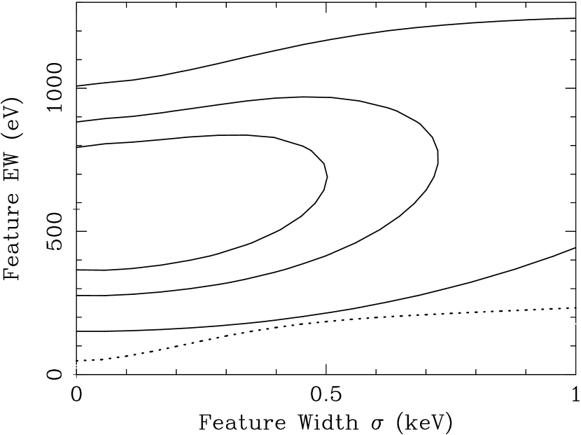
Figure 14: Confidence contours (68%, 90%, & 99%) of EW versus intrinsic width of the 8–9 keV feature for group 5 of the RXTE data for NGC 2992. The 99% confidence, upper limit contour of the feature for quasi-simultaneous Suzaku data is shown as dotted line.

Table 1: NGC 2992 RXTE Observation Log

Obs	Start		End		Exposure	Count Rate
1	04/03/05	13:27:23	04/03/05	14:20:27	6368	10.590 $\pm$ 0.064
2	18/03/05	17:18:35	18/03/05	17:31:07	1504	2.287 $\pm$ 0.106
3	21/03/05	08:16:11	21/03/05	08:54:51	4640	2.730 $\pm$ 0.062
4	05/04/05	10:07:39	05/04/05	10:57:47	4928	7.467 $\pm$ 0.068
5	20/04/05	12:12:27	20/04/05	12:57:47	5440	1.326 $\pm$ 0.055
6	05/05/05	07:37:31	05/05/05	08:28:43	6144	3.646 $\pm$ 0.055
7	08/05/05	06:25:15	08/05/05	07:04:59	4576	3.673 $\pm$ 0.063
8	18/05/05	10:11:15	18/05/05	11:14:43	5216	8.084 $\pm$ 0.068
9	02/06/05	07:32:11	02/06/05	08:16:11	5280	1.555 $\pm$ 0.055
10	16/06/05	06:30:35	16/06/05	07:24:27	6464	1.350 $\pm$ 0.051
11	01/07/05	03:34:35	01/07/05	04:27:55	6400	0.802 $\pm$ 0.050
12	16/07/05	03:57:31	16/07/05	04:35:07	4512	1.203 $\pm$ 0.060
13	29/07/05	03:19:39	29/07/05	04:10:03	6048	3.402 $\pm$ 0.056
14	10/08/05	03:07:55	10/08/05	04:01:31	6432	2.841 $\pm$ 0.053
15	12/09/05	22:44:27	12/09/05	23:35:07	5600	1.882 $\pm$ 0.053
16	27/09/05	00:55:55	27/09/05	01:46:51	6112	1.322 $\pm$ 0.051
17	14/10/05	01:45:31	14/10/05	02:39:07	5600	0.886 $\pm$ 0.055
18	29/10/05	19:13:31	29/10/05	20:03:07	5632	1.013 $\pm$ 0.054
19	13/11/05	22:35:23	13/11/05	23:23:07	5728	1.970 $\pm$ 0.054
20	28/11/05	22:34:03	28/11/05	23:27:23	6400	1.687 $\pm$ 0.051
21	13/12/05	17:55:07	13/12/05	18:45:31	6048	1.827 $\pm$ 0.055
22	28/12/05	19:46:51	28/12/05	20:30:35	5248	1.278 $\pm$ 0.057
23	12/01/06	18:06:34	12/01/06	18:59:54	6400	0.850 $\pm$ 0.051
24	28/01/06	09:52:11	28/01/06	10:45:31	6368	1.882 $\pm$ 0.053

Table 2: NGC 2992 RXTE Fit Results

Obs	F2-10	L2-10	$\Gamma$	$E_{\rm Fe\ K\alpha}$	$\sigma_{\rm Fe\ K\alpha}$	$I_{\rm Fe\ K\alpha}$	EW	$\chi^{2}$	dof
1	8.88	1.17	$1.706^{+0.038}_{-0.039}$	$5.73^{+0.57}_{-0.58}$	$0.83^{+0.55}_{-0.49}$	$18.8^{+10.4}_{-9.6}$	$170^{+94}_{-86}$	20.1	23
			[1.672-1.739]	[ 5.22- 6.23]	[ 0.41- 1.30]	[ 10.3- 27.8]	[ 93- 251]
2	2.00	0.26	$1.812^{+0.292}_{-0.262}$	$6.61^{+0.57}_{-0.58}$	$0.00^{+1.03}_{-0.00}$	$8.9^{+7.7}_{-7.8}$	$464^{+405}_{-406}$	17.5	23
			[1.581-2.066]	[ 6.11- 7.00]	[ 0.00- 0.81]	[ 1.8- 15.6]	[ 94- 817]
3	2.40	0.32	$1.798^{+0.142}_{-0.133}$	$6.53^{+0.57}_{-0.65}$	$0.68^{+0.80}_{-0.68}$	$11.9^{+6.9}_{-6.9}$	$517^{+300}_{-300}$	10.6	23
			[1.681-1.922]	[ 5.98- 7.02]	[ 0.00- 1.35]	[ 5.9- 18.0]	[ 256- 783]
4	6.22	0.82	$1.753^{+0.056}_{-0.058}$	$5.58^{+0.48}_{-0.44}$	$0.68^{+0.71}_{-0.68}$	$20.2^{+9.8}_{-9.3}$	$252^{+122}_{-116}$	17.1	23
			[1.703-1.803]	[ 5.19- 5.99]	[ 0.00- 1.30]	[ 12.0- 28.8]	[ 150- 360]
5	1.17	0.15	$1.814^{+0.246}_{-0.229}$	$6.32^{+0.31}_{-0.29}$	$0.00^{+0.51}_{-0.00}$	$8.2^{+4.1}_{-4.2}$	$710^{+355}_{-363}$	24.1	23
			[1.612-2.029]	[ 6.11- 6.54]	[ 0.00- 0.43]	[ 4.5- 11.8]	[ 389-1022]
6	2.98	0.39	$1.656^{+0.085}_{-0.084}$	$6.10^{+0.43}_{-0.48}$	$0.04^{+1.09}_{-0.04}$	$6.4^{+4.3}_{-4.4}$	$186^{+125}_{-126}$	22.1	23
			[1.582-1.731]	[ 5.70- 6.46]	[ 0.00- 0.98]	[ 2.6- 10.2]	[ 75- 297]
7	2.98	0.39	$1.726^{+0.103}_{-0.101}$	$6.22^{+0.35}_{-0.35}$	$0.33^{+0.57}_{-0.33}$	$11.9^{+5.6}_{-5.6}$	$375^{+176}_{-176}$	20.3	23
			[1.637-1.816]	[ 5.92- 6.53]	[ 0.00- 0.80]	[ 7.0- 16.8]	[ 221- 530]
8	6.66	0.88	$1.688^{+0.062}_{-0.068}$	$5.42^{+0.66}_{-0.68}$	$1.10^{+0.70}_{-0.64}$	$28.5^{+17.7}_{-14.3}$	$297^{+184}_{-149}$	14.3	23
			[1.629-1.743]	[ 4.82- 5.99]	[ 0.53- 1.71]	[ 15.8- 43.8]	[ 164- 456]
9	1.26	0.17	$1.758^{+0.252}_{-0.234}$	$6.16^{+0.65}_{-0.71}$	$0.80^{+0.89}_{-0.80}$	$12.0^{+7.1}_{-7.1}$	$930^{+550}_{-550}$	13.2	23
			[1.554-1.978]	[ 5.55- 6.72]	[ 0.00- 1.54]	[ 5.8- 18.2]	[ 449-1410]
10	1.11	0.15	$1.676^{+0.250}_{-0.234}$	$6.15^{+0.37}_{-0.38}$	$0.59^{+0.53}_{-0.59}$	$13.3^{+5.5}_{-5.4}$	$1189^{+491}_{-482}$	15.7	23
			[1.470-1.894]	[ 5.82- 6.47]	[ 0.00- 1.04]	[ 8.6- 18.1]	[ 768-1618]
11	0.81	0.11	$1.953^{+0.363}_{-0.319}$	$6.30^{+0.59}_{-0.60}$	$0.00^{+1.19}_{-0.00}$	$4.7^{+3.9}_{-3.8}$	$619^{+514}_{-501}$	6.0	23
			[1.670-2.269]	[ 5.80- 6.79]	[ 0.00- 0.98]	[ 1.4- 8.1]	[ 178-1068]
12	0.91	0.12	$1.612^{+0.350}_{-0.324}$	$6.10^{+0.84}_{-0.97}$	$0.55^{+1.01}_{-0.55}$	$7.2^{+6.3}_{-6.2}$	$718^{+628}_{-618}$	15.6	23
			[1.328-1.916]	[ 5.30- 6.80]	[ 0.00- 1.35]	[ 1.8- 12.7]	[ 179-1267]
13	2.88	0.38	$1.774^{+0.099}_{-0.095}$	$6.41^{+0.67}_{-0.74}$	$0.46^{+1.19}_{-0.46}$	$7.1^{+5.3}_{-5.3}$	$243^{+182}_{-182}$	14.8	23
			[1.691-1.861]	[ 5.80- 6.98]	[ 0.00- 1.45]	[ 2.5- 11.8]	[ 85- 405]
14	2.43	0.32	$1.707^{+0.103}_{-0.099}$	$6.27^{+0.36}_{-0.39}$	$0.00^{+1.02}_{-0.00}$	$6.7^{+4.0}_{-4.1}$	$253^{+151}_{-155}$	17.9	23
			[1.620-1.797]	[ 5.95- 6.57]	[ 0.00- 0.89]	[ 3.1- 10.2]	[ 117- 386]
15	1.67	0.22	$1.815^{+0.164}_{-0.155}$	$6.81^{+0.99}_{-2.55}$	$0.00^{+1.94}_{-0.00}$	$3.7^{+3.9}_{-3.7}$	$251^{+265}_{-251}$	17.2	24
			[1.679-1.958]	[ 6.08- 7.42]	[ 0.00- 1.09]	[ 0.4- 7.1]	[ 27- 483]
16	1.14	0.15	$1.774^{+0.260}_{-0.245}$	$6.13^{+0.88}_{-1.06}$	$0.86^{+1.04}_{-0.86}$	$8.9^{+7.1}_{-6.6}$	$764^{+602}_{-568}$	21.4	24
			[1.559-2.001]	[ 5.24- 6.89]	[ 0.00- 1.70]	[ 3.0- 15.1]	[ 256-1290]
17	0.89	0.12	$2.054^{+0.407}_{-0.349}$	$6.38^{+0.31}_{-0.31}$	$0.07^{+0.70}_{-0.07}$	$8.8^{+4.2}_{-4.2}$	$1148^{+557}_{-557}$	22.7	24
			[1.745-2.407]	[ 6.11- 6.65]	[ 0.00- 0.69]	[ 5.0- 12.5]	[ 656-1641]
18	0.85	0.11	$2.075^{+0.423}_{-0.361}$	$6.45^{+0.42}_{-0.41}$	$0.03^{+0.75}_{-0.03}$	$6.3^{+4.2}_{-4.1}$	$876^{+584}_{-570}$	32.5	24
			[1.754-2.442]	[ 6.10- 6.81]	[ 0.00- 0.68]	[ 2.7- 10.0]	[ 375-1391]
19	1.72	0.23	$1.876^{+0.160}_{-0.150}$	$6.27^{+0.39}_{-0.47}$	$0.03^{+1.42}_{-0.03}$	$6.2^{+4.1}_{-4.2}$	$352^{+233}_{-238}$	13.5	24
			[1.744-2.016]	[ 5.88- 6.62]	[ 0.00- 1.22]	[ 2.5- 9.8]	[ 142- 557]
20	0.94	0.12	$2.248^{+0.370}_{-0.315}$	$6.45^{+0.54}_{-0.95}$	$0.40^{+0.89}_{-0.40}$	$6.5^{+4.6}_{-4.6}$	$893^{+625}_{-632}$	27.9	24
			[1.969-2.570]	[ 5.79- 6.92]	[ 0.00- 1.14]	[ 2.5- 10.5]	[ 343-1443]
21	1.52	0.20	$1.834^{+0.212}_{-0.198}$	$6.09^{+0.57}_{-0.62}$	$0.84^{+0.71}_{-0.84}$	$14.2^{+7.5}_{-7.3}$	$915^{+483}_{-470}$	14.1	24
			[1.660-2.020]	[ 5.55- 6.59]	[ 0.00- 1.44]	[ 7.8- 20.8]	[ 502-1340]
22	1.11	0.15	$1.830^{+0.202}_{-0.188}$	$6.40f$	$0.05f$	$2.0^{+3.4}_{-2.0}$	$184^{+305}_{-184}$	22.8	26
			[1.626-2.052]	[…]	[…]	[ 0.0- 5.7]	[ 0- 517]
23	1.28	0.17	$1.746^{+0.136}_{-0.130}$	$6.40f$	$0.05f$	$4.6^{+3.1}_{-3.1}$	$321^{+212}_{-214}$	20.7	26
			[1.605-1.894]	[…]	[…]	[ 1.3- 8.0]	[ 87- 553]
24	1.63	0.22	$1.751^{+0.125}_{-0.119}$	$6.40f$	$0.05f$	$2.5^{+3.2}_{-2.5}$	$148^{+191}_{-148}$	17.2	26
			[1.622-1.887]	[…]	[…]	[ 0.0- 6.0]	[ 0- 355]

Table 3: NGC 2992 RXTE Fit Results: Grouped Data

Group	F2-10	L2-10	$\Gamma$	$E_{\rm Fe\ K\alpha}$	$\sigma_{\rm Fe\ K\alpha}$	$I_{\rm Fe\ K\alpha}$	EW	$\chi^{2}$	dof	P
1	7.38	0.97	$1.713^{+0.029}_{-0.029}$	$5.58^{+0.33}_{-0.33}$	$0.89^{+0.36}_{-0.35}$	$22.3^{+6.8}_{-6.6}$	$232^{+70}_{-68}$	23.6	23	57.7
			[1.688-1.738]	[ 5.29- 5.87]	[ 0.58- 1.20]	[16.5- 28.3]	[ 172- 295]
2	2.70	0.35	$1.723^{+0.045}_{-0.044}$	$6.30^{+0.20}_{-0.20}$	$0.32^{+0.39}_{-0.32}$	$7.7^{+2.2}_{-2.2}$	$271^{+77}_{-77}$	28.2	23	79.3
			[1.684-1.763]	[ 6.13- 6.48]	[ 0.00- 0.66]	[ 5.7- 9.6]	[ 200- 337]
3	1.05	0.14	$1.757^{+0.116}_{-0.112}$	$6.28^{+0.18}_{-0.19}$	$0.26^{+0.38}_{-0.26}$	$7.3^{+2.0}_{-2.0}$	$681^{+186}_{-186}$	27.4	23	76.2
			[1.658-1.859]	[ 6.12- 6.44]	[ 0.00- 0.59]	[ 5.5- 9.1]	[ 513- 849]
4	1.23	0.16	$1.850^{+0.135}_{-0.127}$	$6.45^{+0.33}_{-0.34}$	$0.40^{+0.45}_{-0.40}$	$6.4^{+2.8}_{-2.7}$	$558^{+244}_{-235}$	37.4	24	96.0
			[1.738-1.968]	[ 6.15- 6.74]	[ 0.00- 0.79]	[ 4.0- 8.9]	[ 348- 776]
5	1.25	0.17	$1.961^{+0.123}_{-0.117}$	$6.23^{+0.27}_{-0.30}$	$0.56^{+0.39}_{-0.56}$	$8.6^{+2.9}_{-2.8}$	$718^{+242}_{-233}$	42.9	24	99.0
			[1.858-2.069]	[ 5.96- 6.47]	[ 0.00- 0.91]	[ 6.1- 11.1]	[ 509- 927]
6	1.35	0.18	$1.765^{+0.084}_{-0.081}$	$6.40f$	$0.05f$	$3.1^{+1.9}_{-1.9}$	$215^{+132}_{-132}$	26.8	26	58.2
			[1.677-1.856]	[…]	[…]	[ 1.0- 5.1]	[ 69- 354]
3+4+5	1.17	0.15	$1.861^{+0.070}_{-0.069}$	$6.32^{+0.14}_{-0.14}$	$0.37^{+0.25}_{-0.37}$	$7.3^{+1.4}_{-1.4}$	$642^{+123}_{-123}$	79.4	23	$>4\sigma$
			[1.800-1.923]	[ 6.20- 6.44]	[ 0.00- 0.59]	[ 6.0- 8.5]	[ 528- 748]

References

- Anders & Grevesse (1989) Anders, E., & Grevesse, N. 1989, Geochimica et Cosmochimica Acta 53, 197
- Arnaud (1996) Arnaud, K. A. 1996, in Astronomical Data Analysis Software and Systems V, ed. Jacoby, G., & Barnes, J. (Astronomical Society of the Pacific), Conference Series, Vol. 101, p. 17
- (3) Beckmann, V., Gehrels, N., & Tueller, J. 2007, ApJ in press, astro-ph/0704.2698
- Dickey & Lockman (1990) Dickey, J. M., & Lockman, F. J. 1990, ARA&A, 28, 215
- Dovčiak, Karas, & Yaqoob (2004) Dovčiak, M., Karas, V., & Yaqoob, T. 2004, ApJS, 153, 205
- Fabian (1989) Fabian, A.C., Rees, M.J., Stella, L., & White, N.E. 1989, MNRAS, 238, 729
- Ghisellini, Haardt, & Matt (1994) Ghisellini, G., Haardt, F., & Matt, G. 1994, MNRAS, 267, 743
- Gilli et al. (2000) Gilli, R., Maiolino, R., Marconi, A., Risaliti, G., Dadina, M., Weaver, K. A., & Colbert, E. J. M. 2000, A&A, 355, 485
- Iwasawa et al. (1999) Iwasawa, K., Fabian, A. C., Young, A. J., Inoue, H., & Matsumoto, C. 1999, MNRAS, 306, L19
- Jahoda (2006) Jahoda, K., et al. 2006, ApJS, 163, 401
- mchardy (2007) McHardy, I. M., Koerding, E., Knigge, C., Uttley, P., & Fender, R. P. 2007, Nat, 444, 730
- Markowitz (2004) Markowitz, A., & Edelson, R. 2004, ApJ, 617, 939
- Markowitz (2003) Markowitz, A., Edelson, R., & Vaughan, S. 2003, ApJ, 598, 953
- Mushotzky (1982) Mushotzky, R. F. 1982, ApJ, 256, 92
- Nandra & Pounds (1994) Nandra, K., & Pounds, K. A. 1994, MNRAS, 268, 405
- Palmeri et al. (2003) Palmeri, P., Mendoza, C., Kallman, T. R., & Bautista, M. A. 2003, A&A, 410, 359
- (17) Papadakis, I. E. 2004, MNRAS, 348, 207
- Piccinotti et al. (1982) Piccinotti, G., Mushotzky, R. F., Boldt, E. A., Holt, S. S., Marhsall, F. E., Serlemitsos, P. J., & Shafer, R. A. 1982, ApJ, 253, 485
- Reynolds & Nowak (2003) Reynolds, C. S., & Nowak, M. A. 2003, Pys. Rep., 377, 389
- Rothschild et al. (2006) Rothschild, R. E., et al. 2006, ApJ, 641, 801
- Titarchuk (1994) Titarchuk, L. 1994, ApJ, 434, 570
- Turner & Pounds (1989) Turner, T. J., & Pounds, K. A. 1989, MNRAS, 240, 833
- Turner et al. (1991) Turner, T. J., Weaver, K. A., Mushotzky, R. F., Holt, S. S., & Madejski, G. M. 1991, ApJ, 381, 85
- Turner et al. (1999) Turner, T. J., George, I. M., Nandra, K., & Turcan, D. 1999, ApJ, 524, 667
- Vaughan et al. (2003) Vaughan, S., Edelson, R., Warwick, R. S., & Uttley, P. 2003, ApJ, 345, 1271
- Weaver et al. (1996) Weaver, K. A., Nousek., J., Yaqoob, T., Mushotzky, R. F., Makino, F., & Otani, C. 1996, ApJ, 458, 160
- Woo & Urry (2002) Woo, J. H. & Urry, C. M. 2002, ApJ, 579, 530
- Yaqoob et al. (2001) Yaqoob, T., George, I. M., Nandra, K., Turner, T. J., Serlemitsos, P. J., & Mushotzky, R. F. 2001, ApJ, 546, 759
-
Yaqoob et al. (2007)
Yaqoob, T. et al. 2007, PASJ, in press