A Planetary System Around HD 155358:
The Lowest Metallicity Planet Host Star

Abstract

We report the detection of two planetary mass companions to the solar-type star HD 155358. The two planets have orbital periods of 195.0 and 530.3 days, with eccentricities of 0.11 and 0.18. The minimum masses for these planets are 0.89 and 0.50 M_J respectively. The orbits are close enough to each other, and the planets are sufficiently massive, that the planets are gravitationally interacting with each other, with their eccentricities and arguments of periastron varying with periods of 2300–2700 years. While large uncertainties remain in the orbital eccentricities, our orbital integration calculations indicate that our derived orbits would be dynamically stable for at least $10^{8}$ years. With a metallicity [Fe/H] of -0.68, HD 155358 is tied with the K1III giant planet host star HD 47536 for the lowest metallicity of any planet host star yet found. Thus, a star with only 21% of the heavy-element content of our Sun was still able to form a system of at least two Jovian-mass planets and have their orbits evolve to semi-major axes of 0.6–1.2 AU.

1. Introduction

There is now strongly compelling evidence that planetary companions to main sequence stars are found preferentially around metal-rich stars. Gonzalez (1997, 1998a, 1998b, 1999) was the first to do a detailed comparison of the chemical abundances of stars with and without planets, and to conclude that there was a significant difference in these samples. This finding has subsequently been supported by a large number of investigations, several of which included carefully selected control samples (e.g. Reid, 2002; Heiter & Luck, 2003; Santos et al., 2005; Fischer & Valenti, 2005; Grether & Lineweaver, 2007). Much of the early work in this area concentrated on determining the direction of causality in the observed correlation. That is, does the presence of planets pollute the stellar convective region causing an apparent increase in photospheric metallicity, or does the physics of planet formation significantly favor a metal-rich environment? This issue has been addressed by searching for patterns of elemental enhancement in planet-host stellar photospheres that might result from the metal-rich (or H- and He-poor) detritus of planet formation. So far, there is little compelling evidence that post-formation stellar photospheric self-enrichment is responsible for the observed correlation; a primordial explanation is most likely (Gonzalez, 2006). Thus, searching for planets around stars with relatively low metallicity is extremely important for our understanding of the physics of planet formation. We need to find the lowest metallicity stars around which planets are able to form. The radial-velocity survey of Sozzetti et al. (2006) was the first to specifically target low metallicity stars in order to understand in detail the low-$Z$ end of the dependence of planetary system and formation on metallicity.

We present here the discovery of two planetary companions to the star HD 155358. This is one of the sample of low-metallicity stars that were included in our HET planet survey (Cochran et al., 2004) in order to begin to explore the low-metallicity tail of the heavy element distribution of stars with planets. Details of the observations are given in Section 2. Orbital solutions for the planets are given in Section 3.1 and 3.2. Section 3.3 describes our use of a genetic algorithm to achieve a complete exploration of possible orbital solutions. The dynamical stability of our preferred orbital solution is explored in Section 3.4. Detailed parameters of the host star are given in Section 4, and the implications of this fascinating system for planet formation theories are given in Section 5.

2. Observations

All observations of HD 155358 were made in queue scheduled mode using the High Resolution Spectrometer (Tull, 1998) of the 9.2 m Hobby-Eberly Telescope (Ramsey et al., 1998). A 400µm optical fiber which subtends 2$\farcs$0 on the sky tracks the star across the focal plane of the telescope. Starlight then passes through a molecular iodine absorption cell stabilized at a temperature of 70C. The dense narrow I₂ spectrum which is superimposed on the stellar spectrum enables us to model the instrumental point spread function (Valenti et al., 1995) and provides the velocity metric for precise radial velocity measurement (Butler et al., 1996; Endl et al., 2000). A 250µm spectrograph entrance slit then gives a spectral resolving power of $R=\lambda/\delta\lambda=60,000$. The spectrum is recorded on a mosaic of two $2048\times 4100$ pixel E2V CCDs, which samples the spectrum at $\approx 4$ pixels per resolution element. The cross-disperser is set to obtain the spectrum between 4076Å and 7838Å. A small gap between the two CCDs falls at 5936Å, allowing most of the I₂ absorption spectrum to be recorded on the “blue” CCD chip.

We obtained a total of 71 high signal/noise radial velocity observations of HD 155358 between June 2001 and March 2007. All spectra were processed using standard IRAF routines, and velocities were computed using our high-precision radial velocity code. Table 1 gives the relative radial velocities for HD 155358. The observation times and velocities have been corrected to the solar system barycenter. The uncertainty $\sigma$ for each velocity in the table is an internal error computed from the variance about the mean of the velocities from each of the 480 small chunks into which the spectrum is divided for the velocity computation. Thus, it represents the relative uncertainty of one velocity measurement with respect to the others, based on the quality and observing conditions of the spectrum. This uncertainty does not include other intrinsic stellar sources of uncertainty, nor any unidentified sources of systematic errors.

Table 1Relative Velocities for HD 155358

BJD	Velocity		$\sigma$
-2 400 000	m s-1		m s-1
52071.904837	19.	49	3.28
52075.886827	24.	07	3.17
52076.889856	25.	29	2.93
52091.846435	31.	10	3.08
52422.937143	3.	70	3.43
53189.839130	-30.	67	3.28
53205.795629	-20.	54	3.08
53219.753215	-16.	15	3.35
53498.776977	24.	06	3.72
53507.957634	41.	99	4.30
53507.962870	41.	12	3.81
53511.953195	41.	06	2.88
53512.939314	34.	47	3.29
53590.733229	-13.	27	2.86
53601.700903	-3.	25	2.77
53604.701932	-3.	05	2.97
53606.702997	-5.	41	3.20
53612.684038	3.	44	2.61
53625.645464	29.	05	2.65
53628.624309	28.	41	3.61
53629.619464	23.	41	2.85
53633.616275	20.	48	2.83
53755.042134	-35.	55	4.38
53758.042744	-41.	84	3.70
53765.035558	-30.	94	4.02
53774.021743	-45.	17	4.33
53779.979871	-26.	31	4.27
53805.930694	-5.	23	3.16
53808.892822	-4.	14	4.28
53769.026048	-42.	02	3.56
53866.964277	30.	26	3.87
53869.954988	29.	05	3.55
53881.945116	43.	83	2.66
53889.682359	47.	51	2.83
53894.672403	42.	03	2.80
53897.895406	34.	74	2.39
53898.685344	27.	26	2.75
53899.892253	36.	21	2.91
53902.657932	17.	67	2.53
53903.906452	35.	85	2.87
53904.662338	26.	89	3.03
53905.860234	27.	26	3.10
53907.629415	28.	25	2.75
53908.876910	23.	17	3.05
53910.639802	26.	13	3.61
53911.845252	17.	72	2.70
53912.636138	15.	77	3.03
53917.641443	9.	13	3.12
53924.818858	14.	17	3.21
53925.807994	10.	44	2.60
53926.824657	-0.	29	2.83
53927.822039	9.	12	2.98
53936.790961	-7.	51	2.98
53937.790352	-12.	14	6.01
53937.804652	-0.	17	2.83
53941.762397	-14.	31	2.78
53943.766914	-11.	76	2.83
53954.756895	-10.	92	2.49
53956.734767	-15.	38	2.47
53958.747552	-11.	09	2.50
53960.714843	-9.	99	2.52
53966.708140	-11.	85	2.34
53971.697987	-12.	96	2.51
53985.651466	12.	67	3.81
53988.637456	6.	17	2.83
53990.639454	19.	80	3.29
53993.644925	20.	57	3.27
54136.010987	-17.	45	4.47
54137.005715	-9.	57	3.98
54165.933759	-30.	96	3.73
54167.924067	-24.	81	3.85

3. Orbital Solution

3.1. The First Planet

A periodogram of the HET velocities of HD 155358 show a very strong peak at $\sim$195 days, with substantial additional power in the 300-500 day range. The Scargle (1982) false-alarm probability of this 195-day signal is $4.5\times 10^{-10}$. We first fit a Keplerian orbit to the data using the GaussFit generalized least squares software of Jefferys et al. (1988). This planet, with a period of 193.8 d, eccentricity of 0.16, and K velocity of 31.0 m s^-1 has a minimum mass of $M\sin i=0.79\,$M_J and a semimajor axis of 0.63 AU. The RMS dispersion of the data around the orbital solution is 10.2 m s^-1, and the reduced chi-squared $\chi^{2}_{\nu}=9.67$. This goodness-of-fit parameter is significantly higher than would be expected based, as it is based purely on the internal errors quoted in Table 1. Wright (2005) gives a median “jitter” of 4.4 m s^-1 for main-sequence stars similar to HD 155358. Wright also mentions that subgiants typically have jitters of about 5 m s^-1, as do blue stars (with B-V $<$ 0.6). HD 155358 appears to fall into both categories (cf. section 4, with our derived age of 10 Gyr and Hipparcos B-V=0.545. While some of the additional scatter might be explained as intrinsic stellar velocity variability expected in this star, there is probably some additional source for much of the scatter. Thus, we have searched carefully for additional planets in the system.

3.2. The Second Planet

A Lomb-Scargle periodogram of the residuals around the single-planet orbital fit shows very significant power over a broad range of periods from 200 to 800 days, with the strongest peak around 530 days. The false-alarm probability of this power at 530 days is less than $10^{-6}$. Smaller peaks around 330 days show FAP slightly less than $10^{-3}$. Thus, we investigated the possibility of a second long-period planet HD 155358 c. We used GaussFit to compute simultaneous least-squares solutions of double-Keplerian orbits to the observed velocities. We investigated periods around both 330 days and 530 days. While we were able to find formal Keplerian solutions for both periods, the solutions with P${}_{\rm c}\sim 530$ days gave significantly better fits than did shorter period second planets. When we couple this with the results of our genetic algorithm orbital fits (section 3.3) and dynamical calculations (section 3.4), we have concluded that the 530 day period is correct for HD 155358 c. This solution is given in Table 2 and is shown in Figure 1. The uncertainties reported in Table 2 were generated by GaussFit from a maximum likelihood estimation that is an approximation to a Bayesian maximum a posteriori estimator with a flat prior (Jefferys, 1990). The observed HET velocity residuals to the HD 155358 c fit, phased to the period of HD 155358 b are shown in the upper panel of Figure 2, and vice-versa in the lower panel.

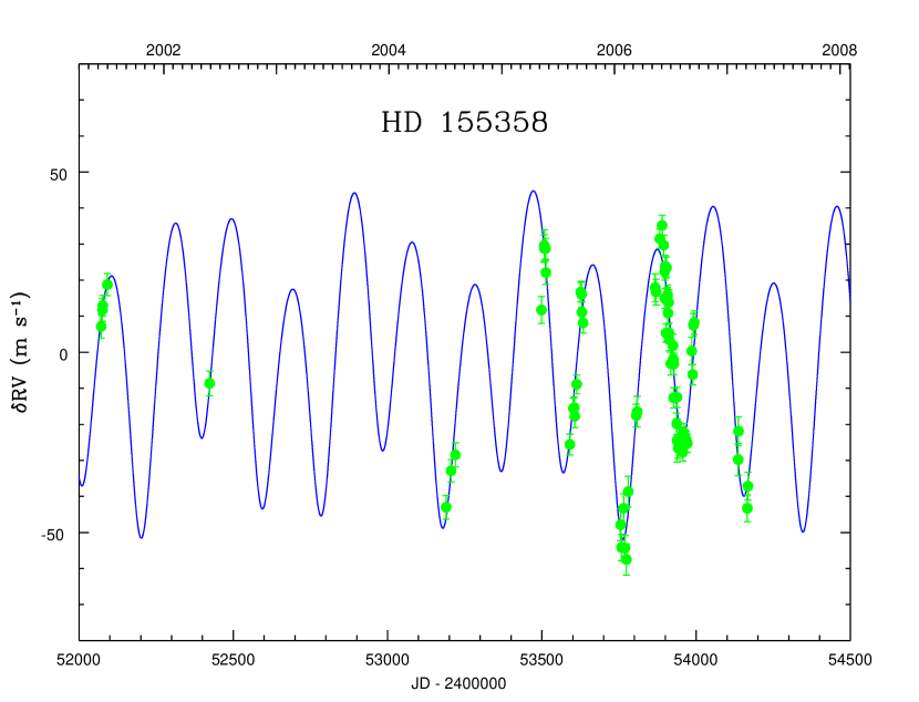
Figure 1.— The HET data velocities of HD 155358 with the best double-planet fit (solid line). The RMS scatter of the data around the fit is 6.0 m s^-1.

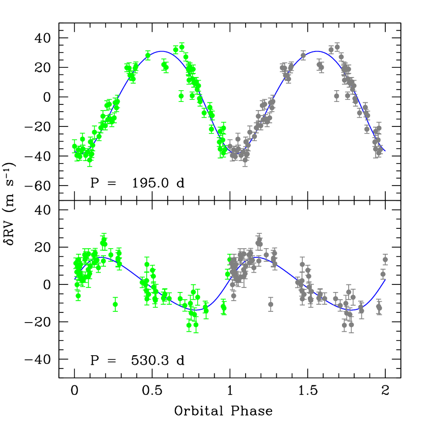
Figure 2.— The best fit double-planet Keplerian orbit solution to the Hobby-Eberly Telescope data for HD 155358. The upper panel shows the phased inner planet (HD 155358 b) orbit, along with the observed data which have had the outer planet (HD 155358 c) orbit removed. The lower panel shows the phased HD 155358 c orbital solution, along with the observed data which have had the the HD 155358 b orbit removed. Two cycles are shown, with the second cycle in grey for clarity. The rms scatter of the data around this double-planet fit is 6.0 m s^-1.

Table 2HD 155358 Double Planet Keplerian Solution

Parameter	Value
Pb	195.0$\pm$	1.1 days
T0b	2453950.0$\pm$	10.4 BJD
Kb	34.6$\pm$	3.0 m s-1
eb	0.112$\pm$	0.037
$\omega_{\rm b}$	162$\pm$	20 degrees
Pc	530.3$\pm$	27.2 days
T0c	2454420.3$\pm$	79.3 BJD
Kc	14.1$\pm$	1.6 m s-1
ec	0.176$\pm$	0.174
$\omega_{\rm c}$	279$\pm$	38 degrees
$M_{\rm b}\sin i$	0.89$\pm$	0.12 $M_{J}$
ab	0.628$\pm$	0.020 AU
$M_{\rm c}\sin i$	0.504$\pm$	0.075 $M_{J}$
ac	1.224$\pm$	0.081 AU
RMS	6.0 m s-1

In fitting a Keplerian orbit to observed data, the eccentricity is often the least well-determined of the orbital elements, and is the one element that is most often able to absorb any additional signals or periodicities that may be in the data. For example, in comparing the HD 155358 b single-planet orbit fit with the elements of HD 155358 b in the two-planet fits, the most significant changes in the orbital elements of HD 155358 b are that the eccentricity dropped somewhat and the K value increased. The uncertainty in the eccentricity of HD 155358 c is rather large. This is probably due to some regions of sparse phase coverage, particularly in the phase intervals 0.30-0.45 and 0.8-1.0. The rms scatter of the observations around this two-planet fit is 6.0 m s^-1. This rms is quite consistent with a stellar internal “jitter” of 4.5 to 5.0 m s^-1 and our typical internal observed velocity uncertainty of 2-4 m s^-1. If we add a stellar “jitter” of 5 m s^-1 in quadrature with the internal errors given in Table 1, we then get a reduced chi-squared for our two-planet fit of 1.15.

3.3. Genetic Algorithm Investigation

In order to understand fully the nature of the orbit of the second planet in this system, we used a standard genetic algorithm to explore further the $\chi^{2}$-landscape of a 2 planet solution and to find possible additional $\chi^{2}$ minima. The initial orbital parameters were distributed randomly over a certain range of start values and during each iteration these parameters were randomly mutated. The solutions “evolve” by using $\chi^{2}$ as the environmental selection mechanism. Solutions that improve $\chi^{2}$ or at least do not degrade it by a certain threshold are allowed to survive and to multiply. Solutions that are above this threshold (e.g. $\chi^{2}<\chi^{2}_{\rm best}$ + 0.1%), and are not able to move back into this $\chi^{2}$ range, are terminated after a few generations (typically 6 generations). Repeating this process many times (each time with new randomly selected starting values) allowed us to probe a much larger parameter space than is usually possible with standard orbital fit programs.

For HD 155358 we performed $>10,000$ trial runs, allowing the period of HD 155358 c to vary between 250 and 2100 days (the time span of observations). We constrained the period of HD 155358 b to the range of 185 to 200 days and its eccentricity to $e_{\rm b}<0.5$.

Three $\chi^{2}$ minima were found by the genetic algorithm: the first with periods for HD 155358 c around 326 days, the second around with P_c 530 days and a third one with P_c around 1540 days. The parameters of the solutions found for the first two minima coincide with the solutions found by GaussFit. However, the third minimum at 1540 days was intriguing, as it represents another possible period for HD 155358 c. A detailed examination of the solutions in this minimum revealed that their eccentricities were all in the range of $0.835$ to $0.86$. With such a high eccentricity the orbits of the two planets would cross and the system would quickly disrupt itself. It appears that this 1540 day solution represents a good formal fit for a physically impossible orbital configuration. In order to further rule out the 1540 days as the true period of the outer planet we performed 1000 additional trials in the period range of 1500 to 1600 days for HD 155358 c and using an upper limit on $e_{\rm c}$ of 0.6. This time no solutions was found with comparable low $\chi^{2}$ values. We thus conclude that the 530 day period is the most likely period for the second planet.

3.4. Dynamical Stability Calculations

While the orbits given in Table 2 represent the least-squares Keplerian orbit solution to the observations, they may not necessarily represent physically realistic orbits for two planets in this system. The inclusion of the second planet HD 155358 c drops the eccentricity of the first planet HD 155358 b slightly, but the new outer planet solution has a somewhat non-zero eccentricity itself. While the orbits for this solution do not cross each other, they do have sufficiently close approaches that the planets may well be interacting dynamically.

To investigate the orbital stability of the two-planet Keplerian orbital solution for the HD 155358 system, we conducted dynamical simulations using the N-body integrator SWIFT. A full description of SWIFT’s capabilities is given by Levison & Duncan (1994). We adopted the stellar mass $M_{*}$=0.87 M_☉ as discussed below in Section 4, and the parameters of the two planets were those given in Table 2. The planets were assumed to be coplanar, and the planet masses were taken to be the minimum values (i.e. $\sin i=1$). All simulations which used shorter period in the range of 300 days discussed above in Section 3.3 for the outer HD 155358 c planet resulted in ejection of one or both planets within $10^{5}$ yr. Thus, we reject all solutions with P_c in the 300 day range. The longer period (P${}_{\rm c}=530.3$ days) for HD 155358 c is favored dynamically, and was used in all subsequent simulations.

The three-body system (star and two planets) was integrated for a total of $10^{8}$ yr. Initial orbits for the planets were taken from Table 2. The system remained stable for the duration of the simulation. As shown in Figure 3, the two planets exchanged eccentricities on a relatively short timescale, with a period of approximately 2700 yr. The eccentricity of planet b varied between 0.02 and 0.18, while the eccentricity of planet c varied between 0.08 and 0.22. The argument of periastron $\omega$ for both planets circulated with a period of about 2300 yr. The two planets spend most of their time with $\left|\omega_{\rm b}-\omega_{\rm c}\right|$ between $120\arcdeg$ and $240\arcdeg$.

Figure 3.— Results of dynamical simulations of the HD 155358 system. The evolution of semimajor axis (a), eccentricity, and the argument of periastron ($\omega$) are shown for a typical $10^{4}$ year interval. The simulation was run for a total of $10^{8}$ years. The two planets exchange eccentricities on a timescale of about 2700 yr, and $\omega$ circulates with a period of about 2300 yr. The semimajor axes of both planets are stable throughout the simulation. These computations were for a star of mass 0.87 M_☉, and planet masses fixed at the minimum mass ($\sin i=1$). However, similar results are obtained for $\sin i\gtrsim 0.4$.

Noting the significant interaction between the two planets in the minimum-mass case, we tested the effect of inclination of the entire system by adjusting the planetary masses and repeating the simulations. More massive planets (sin $i<1$) should interact more strongly with each other, and thus may be less stable. Systems with $\sin i\gtrsim 0.33$ ($i\gtrsim$20°) remained stable for the duration of the tests ($10^{7}$ yr). These results indicate that the dynamical stability evidenced in Figure 3 does not require the special circumstance of a nearly edge-on inclination and thus minimum-mass planets. Even though the two planets are definitely interacting dynamically, the timescale of this interaction is long compared with the span of our observations. Thus, our two-planet least-squares Keplerian solution given in Section 3.2 is a valid approximation.

Throughout the dynamical simulations, we have assumed that the two planets are in coplanar orbits. It is, however, conceivable that the planetary orbits are inclined with respect to each other. We have conducted further tests with mutually inclined planetary orbits to determine the maximum mutual inclination for which the system remained stable. For the purposes of these experiments, the initial inclination of the inner planet was set to $0\arcdeg$ and that of the outer planet was assigned a grid of starting values ranging from $5\arcdeg$ up to $50\arcdeg$. The planetary masses were again assumed to be the minimum values, and the systems were integrated for $10^{7}$ yr. Systems with mutual inclinations less than $45\arcdeg$ remained stable for the duration of the simulations. For higher values of the inclination between the two planets, the eccentricities of both planets experienced chaotic variations resulting in the ejection of the outer planet within $10^{6}$ yr ($45\arcdeg$) and $2\times 10^{5}$ yr ($50\arcdeg$).

4. Stellar Properties

We measured the photospheric iron abundance, [Fe/H], of HD 155358 by analyzing the “template” spectrum used in the radial velocity analysis. We assumed that [Fe/H] was an effective proxy for the general photospheric metallicity, [M/H]. Our analysis method is the same as described by Bean et al. (2006) for solar-type stars. We briefly describe the technique here, and refer the reader to that paper for a complete description.

We fit synthetic spectra to the profiles of 30 Fe I lines in the observed spectrum. We generated the synthetic spectra with an updated version of the plane-parallel, local thermodynamic equilibrium (LTE), stellar analysis computer code MOOG (Sneden, 1973). We assumed astrophysical log gf values for the Fe I lines, which were determined by fitting a solar spectrum and assuming the solar iron abundance log $\epsilon$(Fe)_☉ = 7.45. Our analysis was therefore differential to the sun.

We also adopted model atmospheres computed with the general-purpose stellar atmosphere code PHOENIX (version 13, Hauschildt et al., 1999) for our analysis. The model atmosphere effective temperature, $T_{eff}$, was constrained using the {$(\bv)$, [Fe/H]} – $T_{eff}$ relationship of Ramírez & Meléndez (2005). The surface gravity, log g, was constrained by interpolating the Bertelli et al. (1994) evolutionary isochrones for a given $M_{V}$, $T_{eff}$, and [Fe/H]. We took the needed $V$ magnitude, $(\bv)$ color, and parallax from the Hipparcos catalog (Perryman et al., 1997).

We determined [Fe/H], microturbulence $\xi$, and macroturbulence $\eta$ for HD 155358 by fitting the line profiles in the observed spectrum simultaneously. As the constraints on the stellar $T_{eff}$ and log g described above are both dependent on [Fe/H], these parameters were also varied simultaneously. We fit the observed spectrum by using an adaptation of the “Marquardt” $\chi^{2}$ minimization algorithm (Marquardt, 1963; Press et al., 1986). The uncertainty in the determined [Fe/H] was calculated from the scatter in the abundances determined for each line individually and deviations due to the uncertainties in the adopted $T_{eff}$ and log g.

In addition to the standard spectroscopic parameters, we have also estimated the mass and age of HD 155358 by interpolating the Bertelli et al. (1994) evolutionary isochrones as we did to constrain the log g. The parameters that we determined for HD 155358 are given in Table 3. Table  4 lists the literature values of the stellar parameters for comparison. Most notably, we found [Fe/H] = -0.68 $\pm$ 0.07. This is in very good agreement with the literature values, which have a range -0.72 $\leq$ [Fe/H] $\leq$ -0.60, and median value [Fe/H] = -0.67. The derived value of $\log g$, coupled with the mass, age, and effective temperature of HD 155358 indicate that the star has evolved off the main sequence.

Table 3Derived Stellar Parameters for HD 155358

Parameter	Value
$T_{eff}$	5760$\pm$	101 K
log g	4.09$\pm$	0.10 (cgs)
${\rm[Fe/H]}$	-0.68$\pm$	0.07
$\xi$	1.55$\pm$	0.15 km s-1
$\eta$	1.89$\pm$	0.20 km s-1
$M_{\star}$	0.87$\pm$	0.07 $M_{\sun}$
Age	$\sim$ 10 Gyr

Table 4Stellar Parameters for HD 155358 from Other Sources

$T_{eff}$	log g	[Fe/H]	Mass	Age	Source
(K)	(cgs)		($M_{\sun}$)	(Gyr)
5760	4.09	-0.68	0.87	10.1	1
5870	4.19	-0.67	0.75	$\cdots$	2
5868	4.19	-0.67	$\cdots$	$\cdots$	3
5914	4.09	-0.61	$\cdots$	$\cdots$	4
$\cdots$	$\cdots$	$\cdots$	0.84	10.2	5
5860	4.10	-0.60	$\cdots$	$\cdots$	6
5818	4.09	-0.67	0.89	12.7	7
5888	$\cdots$	-0.69	0.83	13.8	8
$\cdots$	$\cdots$	$\cdots$	$\cdots$	15.7	9
5808	$\cdots$	-0.72	0.89	11.9	10

References. — (1) This Paper, (2) Lambert et al. (1991), (3) Edvardsson et al. (1993), (4) Gratton et al. (1996), (5) Ng & Bertelli (1998), (6) Thévenin & Idiart (1999), (7) Chen et al. (2001), (8) Feltzing et al. (2001), (9) Lambert & Reddy (2004), (10) Nordström et al. (2004)

5. Discussion

The planetary system around HD 155358 is quite remarkable in that it contains two Jovian-mass planets in relatively short-period orbits around one of the most metal-poor planet-host star yet found. Thus, this system is crucial to our understanding of the physics of planetary system formation and early dynamical evolution.

The final configuration of any planetary system results from a competition of several different physical processes, each occurring on its own independent timescale. The planets themselves must form from the remnant disk of material left over from star formation. This must happen before the circumstellar disk is dissipated. After planet formation, the system must evolve into the final state in which we detect it. The dependence of each of these processes on the metallicity of the material from which the entire system forms then determines the range of allowed planetary systems as a function of metallicity.

Matsuo et al. (2007) investigated the circumstances under which stars of various metallicity and mass could form planets within the framework of both the core-accretion model and the disk-instability model. They derive a low metallicity threshold for planet formation within the core accretion model of [Fe/H] = -0.85 for a disk of 5 times the mass of the minimum mass solar nebula (MMSN) and [Fe/H] = -1.17 for a disk of 10 times the MMSN. They also showed that the disk instability model has essentially no dependence on stellar metallicity, but would require a disk mass of at least 10 times the MMSN to form these planets. Thus, the two giant planets we have discovered in the HD 155358 system could have formed from either formation mechanism. In either model they require a disk which was substantially more massive than the minimum-mass solar nebula.

Ida & Lin (2004, 2005) investigated the dependence of the formation of planetary systems on stellar metallicity within the core-accretion model. The motivation for their model was to explain the observed correlation between high stellar metallicity and planetary systems easily detected by RV techniques. The basic idea is that in systems of high metallicity, the dust surface density in the protoplanetary disk will be enhanced. This will lead to planetary cores being formed on a much shorter timescale. Ida & Lin (2005) derived a planetary core mass at time $t$ (prior to depletion of the feeding zone) that is proportional to $10^{3Z}$, where $Z$ is the stellar metallicity ($10^{\rm[Fe/H]_{\star}}Z_{\sun}$). For a giant planet to grow, a core must achieve a mass above a critical value of about 10-20$M_{\oplus}$ before the gas disk is dissipated. If the core does reach a super-critical mass while there is still significant gas content in the disk, it will rapidly accrete gas and grow to become a gas-giant planet. If the core remains sub-critical through gas disk dissipation, then the planetary core will remain a Neptune or a super-Earth. Since the disk dissipation has a much weaker (if any) dependence on stellar metallicity, gas-giant planet formation around low $Z$ stars is significantly more difficult than around stars of solar or higher metallicity. Unless the circumstellar disk is rather massive to begin with, there simply isn’t time to grow critical-mass cores before the gas disk dissipates. Thus, one might expect a critical lower metallicity threshold for the formation of gas giant planets. The value of this threshold would depend on the physics governing the overall mass of the disk, which are poorly understood.

The third relevant timescale for determining the final configuration of a planetary system is that of the planetary system dynamical evolution, which transforms the system from the one which formed the planets into the system which we detect today. There are two basic physical processes governing post-formation dynamical evolution. These are tidal migration prior to disk dissipation, and planet-planet or planet-planetessimal scattering following disk dissipation. Only tidal migration can have any significant dependence on stellar metallicity. The disk evolution is driven by the disk viscosity. In type II migration, in which the planet has opened a gap in the disk as a result of depleting the local gas in the disk from runaway gas accretion, the planet is locked into the viscous evolution of the disk. Ida & Lin (2005) give a disk migration timescale that depends linearly on the disk viscosity, $\alpha$. The dependence of $\alpha$ on metallicity is not known, and most models assume a constant $\alpha$ of order $10^{-4}$ for all disks. Thus, it appears that once a system of several planets is able to form in a disk, the subsequent dynamical evolution of that system is probably reasonably independent of $Z$. Detailed modeling of the dependence of disk evolution and type II migration on $Z$ is needed. If the dynamical evolution of the planetary system is due to tidal migration in the disk, this migration must still occur before the disk is dissipated. If the final configuration of the HD 155358 system is due to post-formation planet-planet scattering, or dynamical interactions of the planets with remnant planetessimals, then we would not necessarily expect any significant dependence of the process on the stellar metallicity. For low metallicity systems, the theoretical challenge is to form the planets of the required mass before the disk dissipates.

References

- Bean et al. (2006) Bean, J. L., Sneden, C., Hauschildt, P. H., Johns-Krull, C. M., & Benedict, G. F. 2006, ApJ, 652, 1604
- Bertelli et al. (1994) Bertelli, G., Bressan, A., Chiosi, C., Fagotto, F., & Nasi, E. 1994, A&AS, 106, 275
- Butler et al. (1996) Butler, R. P., Marcy, G. W., Williams, E., McCarthy, C., Dosanjh, P., & Vogt, S. S. 1996, PASP, 108, 500
- Chen et al. (2001) Chen, Y. Q., Nissen, P. E., Benoni, T., & Zhao, G. 2001, A&A, 371, 943
- Cochran et al. (2004) Cochran, W. D., Endl, M., McArthur, B., Paulson, D. B., Smith, V. V., MacQueen, P. J., Tull, R. G., Good, J., Booth, J., Shetrone, M., Roman, B., Odewahn, S., Deglman, F., Graver, M., Soukup, M., & Villarreal, M. L. 2004, ApJ, 611, L133
- Edvardsson et al. (1993) Edvardsson, B., Andersen, J., Gustafsson, B., Lambert, D. L., Nissen, P. E., & Tomkin, J. 1993, A&A, 275, 101
- Endl et al. (2000) Endl, M., Kürster, M., & Els, S. 2000, A&A, 362, 585
- Feltzing et al. (2001) Feltzing, S., Holmberg, J., & Hurley, J. R. 2001, A&A, 377, 911
- Fischer & Valenti (2005) Fischer, D. A. & Valenti, J. 2005, ApJ, 622, 1102
- Gonzalez (1997) Gonzalez, G. 1997, MNRAS, 285, 403
- Gonzalez (1998a) —. 1998a, A&A, 334, 221
- Gonzalez (1998b) Gonzalez, G. 1998b, in ASP Conf. Ser. 134: Brown Dwarfs and Extrasolar Planets, ed. R. Rebolo, E. L. Martin, & M. R. Z. Osorio, 431
- Gonzalez (1999) —. 1999, MNRAS, 308, 447
- Gonzalez (2006) —. 2006, PASP, 118, 1494
- Gratton et al. (1996) Gratton, R. G., Carretta, E., & Castelli, F. 1996, A&A, 314, 191
- Grether & Lineweaver (2007) Grether, D. & Lineweaver, C. H. 2007, preprint, astro-ph/0612172
- Hauschildt et al. (1999) Hauschildt, P. H., Allard, F., & Baron, E. 1999, ApJ, 512, 377
- Heiter & Luck (2003) Heiter, U. & Luck, R. E. 2003, AJ, 126, 2015
- Ida & Lin (2004) Ida, S. & Lin, D. N. C. 2004, ApJ, 616, 567
- Ida & Lin (2005) —. 2005, Progress of Theoretical Physics Supplement, 158, 68
- Jefferys (1990) Jefferys, W. H. 1990, Biometrika, 77, 597
- Jefferys et al. (1988) Jefferys, W. H., Fitzpatrick, M. J., & McArthur, B. E. 1988, Celestial Mechanics, 41, 39
- Lambert et al. (1991) Lambert, D. L., Heath, J. E., & Edvardsson, B. 1991, MNRAS, 253, 610
- Lambert & Reddy (2004) Lambert, D. L. & Reddy, B. E. 2004, MNRAS, 349, 757
- Levison & Duncan (1994) Levison, H. F. & Duncan, M. J. 1994, Icarus, 108, 18
- Marquardt (1963) Marquardt, D. W. 1963, J. Soc. Ind. Appl. Math., 11, 431
- Matsuo et al. (2007) Matsuo, T., Shibai, H., & Ootsubo, T. 2007, Ap.J. in press, astro-ph/0703237
- Ng & Bertelli (1998) Ng, Y. K. & Bertelli, G. 1998, A&A, 329, 943
- Nordström et al. (2004) Nordström, B., Mayor, M., Andersen, J., Holmberg, J., Pont, E., Jørgensen, B. R., Olsen, E. H., Udry, S., & Mowlavi, N. 2004, A&A, 418, 989
- Perryman et al. (1997) Perryman, M. A. C., Lindegren, L., Kovalevsky, J., Hoeg, E., Bastian, U., Bernacca, P. L., Crézé, M., Donati, F., Grenon, M., van Leeuwen, F., van der Marel, H., Mignard, F., Murray, C. A., Le Poole, R. S., Schrijver, H., Turon, C., Arenou, F., Froeschlé, M., & Petersen, C. S. 1997, A&A, 323, L49
- Press et al. (1986) Press, W. H., Flannery, B. P., & Teukolsky, S. A. 1986, Numerical recipes. The art of scientific computing (Cambridge: University Press, 1986)
- Ramírez & Meléndez (2005) Ramírez, I. & Meléndez, J. 2005, ApJ, 626, 465
- Ramsey et al. (1998) Ramsey, L. W., Adams, M. T., Barnes, T. G., Booth, J. A., Cornell, M. E., Fowler, J. R., Gaffney, N. I., Glaspey, J. W., Good, J. M., Hill, G. J., Kelton, P. W., Krabbendam, V. L., Long, L., MacQueen, P. J., Ray, R. B., Ricklefs, R. L., Sage, J., Sebring, T. A., Spiesman, W. J., & Steiner, M. 1998, Proc. Soc. Photo-opt. Inst. Eng., 3352, 34
- Reid (2002) Reid, I. N. 2002, PASP, 114, 306
- Santos et al. (2005) Santos, N. C., Israelian, G., Mayor, M., Bento, J. P., Almeida, P. C., Sousa, S. G., & Ecuvillon, A. 2005, A&A, 437, 1127
- Scargle (1982) Scargle, J. D. 1982, ApJ, 263, 835
- Sneden (1973) Sneden, C. A. 1973, PhD Thesis, The University of Texas at Austin
- Sozzetti et al. (2006) Sozzetti, A., Torres, G., Latham, D. W., Carney, B. W., Stefanik, R. P., Boss, A. P., Laird, J. B., & Korzennik, S. G. 2006, ApJ, 649, 428
- Thévenin & Idiart (1999) Thévenin, F. & Idiart, T. P. 1999, ApJ, 521, 753
- Tull (1998) Tull, R. G. 1998, Proc. Soc. Photo-opt. Inst. Eng., 3355, 387
- Valenti et al. (1995) Valenti, J. A., Butler, R. P., & Marcy, G. W. 1995, PASP, 107, 966
- Wright (2005) Wright, J. T. 2005, PASP, 117, 657