Polariton-polariton scattering :
exact results through a novel approach

Abstract

We present a fully microscopic approach to the transition rate of two exciton-photon polaritons. The non-trivial consequences of the polariton composite nature — here treated exactly through a development of our composite-exciton many-body theory — lead to results noticeably different from the ones of the conventional approaches in which polaritons are mapped into elementary bosons. Our work reveals an appealing fundamental scattering which corresponds to a photon-assisted exchange — in the absence of Coulomb process. This scattering being dominant when one of the scattered polaritons has a strong photon character, it should be directly accessible to experiment. In the case of microcavity polaritons, it produces a significant enhancement of the polariton transition rate when compared to the one coming from Coulomb interaction. This paper also contains the crucial tools to securely tackle the many-body physics of polaritons, in particular towards its possible BEC.

PACS :

71.36.+c Polaritons

71.35.-y Excitons and related phenomena

71.35.Lk Collective effects (Bose effects, phase space filling, and excitonic phase transitions)

Almost 50 years ago, J.J. Hopfield [1] has shown that photons can be dressed by semiconductor excitations to form a mixed state, the polariton. As this mixed state is the exact eigenstate of the coupled photon-semiconductor Hamiltonian, semiconductor should not absorb any photon. Actually, photon absorption is observed when the exciton broadening is large compared to the exciton-photon coupling. The absorption then follows the Fermi golden rule in spite of the fact that the transition is not towards a continuum, but a discrete state, namely, the exciton with a center-of-mass momentum equal to the photon momentum. This can be physically understood by saying that the exciton broadening acts as a continuum around the exciton discrete level [2].

In the most basic approach to polaritons [3,4], the excitons are considered as non-interacting elementary bosons: The polariton effect then is a bare one-photon one-exciton effect, independent from the laser intensity. This has to be contrasted with the exciton optical Stark effect discovered 25 years ago by D. Hulin and coworkers [5,6], in which the observed exciton line shift, proportional to the laser intensity, only comes from excitons differing from elementary bosons. This apparent contradiction in problems quite similar, namely, photons interacting with a semiconductor, has been tackled by one of us [7] : Through the derivation of the polariton effect and the exciton optical Stark effect within the same framework, it is possible to show that the polariton picture with excitons as non-interacting elementary bosons, is valid at low laser intensity, while the composite nature of the excitons becomes crucial when the laser intensity gets large.

We have recently constructed a many-body theory for excitons in which the composite nature of the particles is treated exactly. It has, up to now, been developed through more than 30 publications. This leads us to consider that the reader now has some knowledge of this many-body theory, at least through the short review paper [8] or, for more details, through the appendices of ref. [9]. The most important result of this theory is the fact that excitons interact not only through Coulomb scatterings for interactions between their carriers, but also through “Pauli scatterings” for carrier exchanges in the absence of Coulomb process. It turns out that these dimensionless pure carrier exchanges — which are by construction missed in effective Hamiltonians for boson excitons, due to a bare dimensional argument, — dominate all semiconductor optical nonlinearities. Among these nonlinear effects, we can cite the exciton optical Stark shift [6] extensively studied in the 80’s. We can also cite the Faraday rotation in photoexcited semiconductors that we have recently suggested [10]. More generally, through a novel approach to the nonlinear susceptibility [11], we have proved that the large detuning behavior of $\chi^{(3)}$ is entirely controlled by these pure carrier exchanges between composite excitons. Processes in which Coulomb interactions take place only enter as detuning corrections.

An “ideal” polariton made of non-interacting boson excitons and (non-interacting boson) photons, would behave as a non-interacting boson. In order to explain the observed scatterings between polaritons, it is necessary to take into account the fact that excitons do interact. To possibly treat their interactions through available many-body procedures — valid for elementary quantum particles only [12,13], — excitons are commonly considered as elementary bosons, their composite nature being hidden through the Coulomb exchange term of the exciton-exciton scattering in the exciton effective Hamiltonian generated by the “bosonization” procedure. In previous works, we have shown that not only the effective exciton-exciton scattering up to now used [14] should have been rejected long ago because it induces an unphysical non hermiticity in the effective exciton Hamiltonian [15], but, worse, there is no way to properly treat the interactions between excitons through an effective potential between elementary bosons, whatever the exciton-exciton scatterings are [9,16]. All our works on exciton many-body effects end with the same conclusion : It is not possible to forget the composite nature of the excitons by reducing them to elementary bosons, whatever the bosonization procedure is.

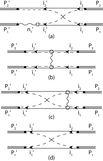
Figure 1: (a): Photon-assisted exchange scattering of two polaritons $\chi\left({}^{P^{\prime}_{2}\ P_{2}}_{P^{\prime}_{1}\ P_{1}}\right)$. (b): Direct Coulomb scattering of two polaritons $\tilde{\xi}^{\mathrm{dir}}\left({}^{P^{\prime}_{2}\ P_{2}}_{P^{\prime}_{1}\ P_{1}}\right)$. (c): “In” exchange Coulomb scattering of two polaritons $\tilde{\xi}^{\mathrm{in}}\left({}^{P^{\prime}_{2}\ P_{2}}_{P^{\prime}_{1}\ P_{1}}\right)$. (d): Pauli scattering of two polaritons $\tilde{\lambda}\left({}^{P^{\prime}_{2}\ P_{2}}_{P^{\prime}_{1}\ P_{1}}\right)$.

The present work on polariton-polariton scatterings once more supports this conclusion. Our composite-exciton many-body theory reveals the existence of an appealing “photon-assisted exchange” channel in the scattering of two polaritons which directly comes from the exciton composite nature (see fig.1(a)) : In this channel, the excitonic parts $i_{1}$ and $i_{2}$ of the polaritons $P_{1}$ and $P_{2}$ exchange their carriers without any Coulomb process. In a second step, one of the resulting excitons, let us say $i^{\prime}_{1}$, transforms into the photon part $n^{\prime}_{1}$ of the polariton $P^{\prime}_{1}$ through the vacuum Rabi coupling, so that this photon-assisted exchange scattering also is an energy-like quantity in spite of the absence of Coulomb process. When compared to the two other channels of the standard approach to polariton-polariton scattering, associated to direct and exchange Coulomb interaction between the excitonic parts of the polaritons (see figs.1(b,c))), this photon-assisted exchange scattering is obviously going to be dominant when one of the four polaritons has a strong photon character, the photon-polariton overlap being then larger than the exciton-polariton overlap. This makes it directly accessible to experiments.

Microscopic formalism

The Hamiltonian of a semiconductor coupled to a photon field splits as $H=H_{\mathrm{ph}}+H_{\mathrm{sc}}+H_{\mathrm{ph-sc}}$. The photon part reads $H_{\mathrm{ph}}=\sum_{n}\omega_{n}a_{n}^{\dagger}a_{n}$ where $a_{n}^{\dagger}$ creates a photon in a mode $n$. The semiconductor part, $H_{\mathrm{sc}}=H_{e}+H_{h}+V_{ee}+V_{hh}+V_{eh}$, contains kinetic and Coulomb contributions for free carriers. Its one-electron-hole-pair eigenstates, $(H_{\mathrm{sc}}-E_{i})B_{i}^{\dagger}|v\rangle=0$, are the excitons, their bound and extended states forming a complete basis for one-pair states. For photons close to the exciton resonance, the photon-semiconductor coupling, $H_{\mathrm{ph-sc}}=W+W^{\dagger}$, can be reduced to its resonant terms, $W=\sum_{n,i}\Omega_{ni}\,\alpha_{n}^{\dagger}B_{i}$, where $\Omega_{ni}$ is the vacuum Rabi coupling between the $n^{\mathrm{th}}$ photon mode and the $i^{\mathrm{th}}$ exciton: $W$ creates a photon while destroying an exciton.

Polaritons $C_{P}^{\dagger}|v\rangle$ are the $H$ eigenstates in the subspace made of one photon coupled to one exciton, $(H-\mathcal{E}_{P})C_{P}^{\dagger}|v\rangle=0$. They thus form a complete orthogonal basis for this subspace. Consequently, we can write photons and excitons in terms of polaritons as

$$a_{n}^{\dagger}=\sum_{P}C_{P}^{\dagger}\,\alpha_{Pn}\ ,\ \ \ \ B_{i}^{\dagger}=\sum_{P}C_{P}^{\dagger}\,\beta_{Pi}\ ,$$ (1)

while polaritons read in terms of photons and excitons as

$$C_{P}^{\dagger}=\sum_{n}a_{n}^{\dagger}\,\alpha_{nP}+\sum_{i}B_{i}^{\dagger}\,\beta_{iP}\ .$$ (2)

The prefactors in these expansions are nothing but the Hopfield coefficients, i.e., the photon-polariton overlap $\alpha_{nP}=\langle v|a_{n}C_{P}^{\dagger}|v\rangle=\alpha_{Pn}^{\ast}$ and the exciton-polariton overlap $\beta_{iP}=\langle v|B_{i}C_{P}^{\dagger}|v\rangle=\beta_{Pi}^{\ast}$. They can be made large or small depending on the polariton character.

Elementary scatterings between polaritons

Due to their excitonic components, the polaritons are not exact bosons. This is readily seen from $[C_{P^{\prime}},C_{P}^{\dagger}]=\delta_{P^{\prime},P}-\tilde{D}_{P^{\prime}P}$, where $\tilde{D}_{P^{\prime}P}$ is the “polariton deviation-from-boson operator”. Using eqs. (1,2), $\tilde{D}_{P^{\prime}P}$ is just the exciton deviation-from-boson operator $D_{i^{\prime}i}$ of the composite-exciton many-body theory (see eq. (1.3) of ref. [9]), dressed by photons through the exciton-polariton overlaps, namely, $\tilde{D}_{P^{\prime}P}=\sum_{i^{\prime},i}\beta_{P^{\prime}i^{\prime}}\,\,D_{i^{\prime}i}\,\beta_{iP}$. The Pauli scatterings of two polaritons $\tilde{\lambda}$, resulting from fermion exchanges as shown in fig.1(d), appear through

$$\left[\tilde{D}_{P^{\prime}_{1}P_{1}},C_{P_{2}}^{\dagger}\right]=\sum_{P^{\prime}_{2}}C_{P^{\prime}_{2}}^{\dagger}\left\{\tilde{\lambda}\left({}^{P^{\prime}_{2}\ P_{2}}_{P^{\prime}_{1}\ P_{1}}\right)+(P_{1}\leftrightarrow P_{2})\right\}\ .$$ (3)

These scatterings are just the exciton Pauli scatterings $\lambda$ of the composite-exciton many-body theory (see eq. (1.2) of ref. [9]), dressed by photons

$$\tilde{\lambda}\left({}^{P^{\prime}_{2}\ P_{2}}_{P^{\prime}_{1}\ P_{1}}\right)=\sum_{i^{\prime}_{1},i^{\prime}_{2},i_{1},i_{2}}\beta_{P^{\prime}_{1}i^{\prime}_{1}}\beta_{P^{\prime}_{2}i^{\prime}_{2}}\,\lambda\left({}^{i^{\prime}_{2}\ i_{2}}_{i^{\prime}_{1}\ i_{1}}\right)\,\beta_{i_{2}P_{2}}\beta_{i_{1}P_{1}}\ .$$ (4)

As for excitons [9], it is not possible to describe the interactions between polaritons through a potential, due to the composite nature of the excitonic part of these polaritons. The clean way to overcome this difficulty is to introduce the “creation-potential” of the polariton $P$, defined as

$$[H,C_{P}^{\dagger}]-\mathcal{E}_{P}C_{P}^{\dagger}=\tilde{V}_{P}^{\dagger}-X_{P}^{\dagger}\ .$$ (5)

Its first part $\tilde{V}_{P}^{\dagger}$ barely is the exciton creation-potential $V_{i}^{\dagger}$ coming from Coulomb interaction between excitons (see eq. (1.7) of ref. [9]), dressed by photons, $\tilde{V}_{P}^{\dagger}=\sum_{i}V_{i}^{\dagger}\,\beta_{iP}$. The second part $X_{P}^{\dagger}$ is conceptually new. It comes from the composite nature of the excitons, through the exciton deviation-from-boson operator $D_{i^{\prime}i}$

$$X_{P}^{\dagger}=\sum_{n,i^{\prime},i}a_{n}^{\dagger}\,\Omega_{ni^{\prime}}\,D_{i^{\prime}i}\,\beta_{iP}\ .$$ (6)

These two creation-potentials give rise to two physically different scatterings. The ones associated to $\tilde{V}_{P}^{\dagger}$,

$$\left[\tilde{V}_{P_{1}}^{\dagger},C_{P_{2}}^{\dagger}\right]=\sum_{P^{\prime}_{1},P^{\prime}_{2}}C_{P^{\prime}_{1}}^{\dagger}C_{P^{\prime}_{2}}^{\dagger}\,\tilde{\xi}^{\mathrm{dir}}\left({}^{P^{\prime}_{2}\ P_{2}}_{P^{\prime}_{1}\ P_{1}}\right)\ ,$$ (7)

shown in Fig.1(b), are naïve. They just correspond to the exciton direct Coulomb scatterings $\xi^{\mathrm{dir}}$ (see eq. (1.8) in ref. [9]), dressed by photons as in eq. (4),

$$\tilde{\xi}^{\mathrm{dir}}\left({}^{P^{\prime}_{2}\ P_{2}}_{P^{\prime}_{1}\ P_{1}}\right)=\sum_{i^{\prime}_{1},i^{\prime}_{2},i_{1},i_{2}}\beta_{P^{\prime}_{1}i^{\prime}_{1}}\beta_{P^{\prime}_{2}i^{\prime}_{2}}\,\xi^{\mathrm{dir}}\left({}^{i^{\prime}_{2}\ i_{2}}_{i^{\prime}_{1}\ i_{1}}\right)\,\beta_{i_{2}P_{2}}\beta_{i_{1}P_{1}}\ .$$ (8)

The ones associated to the second creation-potential $X_{P}^{\dagger}$ are more interesting. They correspond to the photon-assisted exchange scatterings dexcribed in the introduction and shown in fig.1(a). Being defined through

$$\left[X_{P_{1}}^{\dagger},C_{P_{2}}^{\dagger}\right]=\sum_{P^{\prime}_{1},P^{\prime}_{2}}C_{P^{\prime}_{1}}^{\dagger}C_{P^{\prime}_{2}}^{\dagger}\left\{\chi\left({}^{P^{\prime}_{2}\ P_{2}}_{P^{\prime}_{1}\ P_{1}}\right)+(P_{1}\leftrightarrow P_{2})\right\}\ ,$$ (9)

their mathematical expression is

$$\chi\left({}^{P^{\prime}_{2}\ P_{2}}_{P^{\prime}_{1}\ P_{1}}\right)=\sum_{n^{\prime}_{1},i^{\prime}_{1},i^{\prime}_{2},i_{1},i_{2}}\hskip 113.81102pt$$

$$\beta_{P^{\prime}_{2}i^{\prime}_{2}}\alpha_{P^{\prime}_{1}n^{\prime}_{1}}\Omega_{n^{\prime}_{1}i^{\prime}_{1}}\lambda\left({}^{i^{\prime}_{2}\ i_{2}}_{i^{\prime}_{1}\ i_{1}}\right)\,\beta_{i_{1}P_{1}}\beta_{i_{2}P_{2}}\ .$$ (10)

They read in terms of the exciton pure exchange Pauli scatterings $\lambda$, without any Coulomb process.

The two energy-like scatterings $\tilde{\xi}^{\mathrm{dir}}\left({}^{P^{\prime}_{2}\ P_{2}}_{P^{\prime}_{1}\ P_{1}}\right)$, $\chi\left({}^{P^{\prime}_{2}\ P_{2}}_{P^{\prime}_{1}\ P_{1}}\right)$ and the dimensionless Pauli scattering $\tilde{\lambda}\left({}^{P^{\prime}_{2}\ P_{2}}_{P^{\prime}_{1}\ P_{1}}\right)$ this procedure generates, constitute the crucial tools to, in the future, tackle any problem dealing with the many-body physics of polaritons, with the exciton composite nature included in an exact way. This is going to be of importance in view of the claimed recent observation of the polariton BEC [17,18].

Polariton transition rate

To get the polariton transition rate, we barely follow the procedure we have already used to get the exciton transition rate [9,16]. When $H$ does not split as $H_{0}+V$, the standard form of the Fermi golden rule cannot be used. The transition rate from a normalized state $|\phi_{i}\rangle$ to a normalized state $|\phi_{f}\rangle$, is then obtained through [16]

$$\frac{t}{T_{i\rightarrow f}}=\left|\langle\phi_{f}|F_{t}(\hat{H})P_{\perp}H|\phi_{i}\rangle\right|^{2}\ ,$$ (11)

with $P_{\perp}=1-|\phi_{i}\rangle\langle\phi_{i}|$ and $\hat{H}=H-\langle\phi_{i}|H|\phi_{i}\rangle$, while $|F_{t}(E)|^{2}=2\pi\,t\,\delta_{t}(E)$ where $\delta_{t}(E)=(\sin Et/2)/\pi E$ is a peaked function of width $2/t$.

We here consider the transition rate of two identical polaritons $P$ towards two polaritons $(P_{1},P_{2})$. To normalize the initial state $C_{P}^{{\dagger}2}|v\rangle$ and the scattered state $C_{P_{1}}^{\dagger}C_{P_{2}}^{\dagger}|v\rangle$, we use

$$\langle v|C_{P^{\prime}_{1}}C_{P^{\prime}_{2}}C_{P_{2}}^{\dagger}C_{P_{1}}^{\dagger}|v\rangle=\delta_{P^{\prime}_{1},P_{1}}\,\delta_{P^{\prime}_{2},P_{2}}-\tilde{\lambda}\left({}^{P^{\prime}_{2}\ P_{2}}_{P^{\prime}_{1}\ P_{1}}\right)$$

$$+\ (P_{1}\leftrightarrow P_{2})\ ,$$ (12)

which follows from eq. (3).

The transition rate from $(P,P)$ to $(P_{1},P_{2})$, given in eq. (11), makes use of $P_{\perp}HC_{P}^{{\dagger}2}|v\rangle$. To get it, we note that, due to eqs. (5,7,9), $|S_{P}\rangle=(H-2\mathcal{E}_{P})C_{P}^{{\dagger}2}|v\rangle$ reads in terms of the two elementary scatterings of the polariton many-body theory as

$$|S_{P}\rangle=\sum_{P^{\prime}_{1},P^{\prime}_{2}}\left\{\tilde{\xi}^{\mathrm{dir}}\left({}^{P^{\prime}_{2}\ P}_{P^{\prime}_{1}\ P}\right)-2\chi\left({}^{P^{\prime}_{2}\ P}_{P^{\prime}_{1}\ P}\right)\right\}C_{P^{\prime}_{1}}^{\dagger}C_{P^{\prime}_{2}}^{\dagger}|v\rangle\ .$$ (13)

As $P_{\perp}C_{P}^{{\dagger}2}|v\rangle=0$, this makes $P_{\perp}HC_{P}^{{\dagger}2}|v\rangle$, equal to $P_{\perp}|S_{P}\rangle$, linear in polariton scatterings — its precise value being $[|S_{P}\rangle-|S^{\prime}_{P}\rangle]$ with $|S^{\prime}_{P}\rangle=\xi_{P}C_{P}^{{\dagger}2}|v\rangle$, where $\xi_{P}=\langle v|C_{P}^{2}|S_{P}\rangle\langle v|C_{P}^{2}C_{P}^{{\dagger}2}|v\rangle^{-1}$. Consequently, to get the transition rate from $(P,P)$ to $(P_{1},P_{2})\neq(P,P)$ at lowest order in the interactions, we just have, in eq. (11), to replace $\hat{H}$ by its zero order contribution, i.e., $\hat{H}$ by $(\mathcal{E}_{P_{1}}+\mathcal{E}_{P_{2}}-2\mathcal{E}_{P})$ in $\langle v|C_{P_{2}}C_{P_{1}}F_{t}(\hat{H})$. We then note that, for a large sample, the $\tilde{\lambda}$’s, as the exciton Pauli scatterings $\lambda$, are small compared to 1. This makes the $\tilde{\lambda}$’s in the normalization factors negligible as well as the contribution coming from $|S^{\prime}_{P}\rangle$. This allows to show that the transition rate from polaritons $(P,P)$ to polaritons $(P_{1},P_{2})$ reduces to [19]

$$\frac{1}{T_{PP\rightarrow P_{1}P_{2}}}\simeq 4\pi\,\delta_{t}(\mathcal{E}_{P_{1}}+\mathcal{E}_{P_{2}}-2\mathcal{E}_{P})\hskip 85.35826pt$$

$$\times\left|\tilde{\xi}^{\mathrm{dir}}\left({}^{P_{2}\ P}_{P_{1}\ P}\right)-\tilde{\xi}^{\mathrm{in}}\left({}^{P_{2}\ P}_{P_{1}\ P}\right)-\chi\left({}^{P_{2}\ P}_{P_{1}\ P}\right)-\chi\left({}^{P_{1}\ P}_{P_{2}\ P}\right)\right|^{2}\ .$$ (14)

$\tilde{\xi}^{\mathrm{in}}$, the diagram of which is shown in fig.(1c), is the exciton “in” Coulomb exchange scattering $\xi^{\mathrm{in}}$ of the composite-exciton many-body theory (see eq. (1.10) in ref. [9]), dressed by photons as in eq. (8).

Equation (14) for the polariton transition rate is one of the key results of the paper. This transition rate conserves energy at the scale $1/t$, as expected. Its amplitude contains direct and “in” exchange Coulomb scatterings similar to the ones we found for the exciton transition rate [9,16]. However, it contains in addition a contribution from the photon-assisted exchange channel, independent from any Coulomb process. This physically appealing contribution is directly linked simultaneously to the exciton composite nature and to the partly photon nature of the polariton.

State of the art

In the most naïve approach to polariton-polariton scattering, one just replaces the excitons in the photon-semiconductor coupling $W$ by elementary bosons $\bar{B}_{i}$ with $[\bar{B}_{i},\bar{B}_{j}^{\dagger}]=\delta_{i,j}$ and the semiconductor Hamiltonian by an effective exciton-exciton Hamiltonian. If the effective scattering $\xi^{\mathrm{dir}}\left({}^{n\ \,j}_{m\ i}\right)-\xi^{\mathrm{out}}\left({}^{n\ \,j}_{m\ i}\right)$, derived by Haug and Schmitt-Rink [14], were used, the bracket in the polariton transition rate (14) would be $\tilde{\xi}^{\mathrm{dir}}\left({}^{P^{\prime}_{2}\ P}_{P^{\prime}_{1}\ P}\right)-\tilde{\xi}^{\mathrm{out}}\left({}^{P^{\prime}_{2}\ P}_{P^{\prime}_{1}\ P}\right)$. Besides the fact that $\xi^{\mathrm{in}}\neq\xi^{\mathrm{out}}$ (for a complete discussion, see ref. [9]), this procedure totally misses the photon-assisted exchange scattering $\chi$ which is dominant when one of the two scattered polaritons has a strong photon character.

A more elaborate approach, which relies on a truncated Usui’s bosonization procedure, has been proposed by the Quattropani’s group [20,21]. Their Coulomb contribution is now correct (the prefactors of eq. (18) in ref. [20], given in their eqs. (19,20), being nothing but $\xi^{\mathrm{dir}}-\xi^{\mathrm{in}}$). They also find a second contribution called therein “anharmonic saturation term” (see eq. (15) in ref. [20] or the third equation of ref. [21]). Due to the $a^{\dagger}\bar{B}^{\dagger}\bar{B}\bar{B}$ structure of the interaction from which it appears, we could think it to be the photon-assisted exchange channel we find. However, when considered carefully, the physics it bares is at odd. This can be seen seen from the prefactor $Y$ of the interaction term, eq. (15) of ref. [20], explicitly given in eq. (16): It contains the cube of the exciton relative motion wave function. The three wave functions barely come from the three boson-exciton operators of $a^{\dagger}\bar{B}^{\dagger}\bar{B}\bar{B}$. Since the exciton-photon vacuum Rabi coupling also depends on the exciton wave function, their exciton saturation density $n_{sat}$ as defined in ref. [21], ends by reading

$$\frac{1}{n_{sat}L^{2}}=\frac{2\sum_{\mathbf{k}}\phi_{0}^{3}(\mathbf{k})}{\sum_{\mathbf{k}}\phi_{0}(\mathbf{k})}=\frac{4\pi}{7}\left(\frac{a_{X}}{L}\right)^{2}\ ,$$ (15)

where $\phi_{0}(\mathbf{k})=\langle\mathbf{k}|\nu_{0}\rangle$ is the 2D ground state exciton wave function equal to $\sqrt{2\pi}[1+(ka_{X}/2)^{2}]^{-3/2}a_{X}/L$, with $a_{X}$ being the 3D Bohr radius and $L^{2}$ the well area.

On the opposite, in our photon-assisted exchange scattering $\chi$, enters the exciton Pauli scattering. For ground state exciton with zero center-of-mass momentum, it reads [22]

$$\lambda\left({}^{\nu_{0}\mathbf{0}\ \nu_{0}\mathbf{0}}_{\nu_{0}\mathbf{0}\ \nu_{0}\mathbf{0}}\right)=\sum_{\mathbf{k}}\phi_{0}^{4}(\mathbf{k})=\frac{4\pi}{5}\left(\frac{a_{X}}{L}\right)^{2}\ .$$ (16)

Therefore we see that the photon-assisted exchange scattering $\chi$ has to definitely contain the $4^{\mathrm{th}}$ power of the exciton wave function, due to the four excitons involved in the carrier exchange linked with this channel. Since ref. [20] is very elliptical with respect to the derivation of their interaction Hamiltonian, we cannot point out the origin of the incorrectness.

Microcavity polaritons

We end this work on polaritons by considering a specific example, microcavity polaritons, as they are of high current interest for the possible observation of Bose-Einstein condensation of semiconductor excitations [17,18].

In microcavities, the excitons are localized in quantum well. In the strong confinement regime, they are quasi-2D excitons; their energy simply reads $E_{\nu\mathbf{q}}=(E_{g}+\varepsilon_{ze}+\varepsilon_{zh}+\epsilon_{\nu}+\hbar^{2}q^{2}/2M_{X})$, where $\mathbf{q}$ is the 2D exciton center-of-mass momentum. To get the polariton scatterings from the exciton scatterings, we first need to determine the exciton-polariton and photon-polariton overlaps. To do so, we note that, for a single photon mode $n=\mathbf{q}$ close to the ground state exciton resonance, we can forget the higher quantum well subbands as well as the exciton excited levels, so that the excitons of interest reduce to $i=(\nu_{0},\mathbf{q})$. Due to momentum conservation in the exciton-photon coupling, the eigenvalue equation for the polariton $(P_{\mathbf{q}},\mathcal{E}_{\mathbf{q}})$ then reduces to a $2\times 2$ matrix

$$\left(\begin{array}[]{cc}E_{\nu_{0}\mathbf{q}}-\mathcal{E}_{\mathbf{q}}&\Omega^{\ast}_{\mathbf{q}}\\ \Omega_{\mathbf{q}}&\omega_{\mathbf{q}}-\mathcal{E}_{\mathbf{q}}\end{array}\right)\left(\begin{array}[]{c}\beta_{\nu_{0}\mathbf{q},P_{\mathbf{q}}}\\ \alpha_{\mathbf{q},P_{\mathbf{q}}}\end{array}\right)=0\ ,$$ (17)

where $\omega_{\mathbf{q}}=\sqrt{(k^{2}+q^{2})c^{2}/\epsilon}$ is the cavity photon energy with $k=\pi/L_{cav}$ for an optical cavity length $L_{cav}$. The vacuum Rabi coupling between the cavity photon with energy $\omega_{\mathbf{q}}$ and the ground state exciton $(\nu_{0}\mathbf{q})$ located in the well reduces to $\Omega_{\mathbf{q}}=\Omega_{0}\sqrt{\omega_{\mathbf{0}}/\omega_{\mathbf{q}}}$. Typical values for InGaAs/GaAs microcavities are $\omega_{\mathbf{0}}\simeq E_{\nu_{0}\mathbf{0}}\simeq$ 1.5 eV, $\Omega_{0}\simeq 4$ meV, while $m_{e}\simeq 0.067$, $m_{h}\simeq 0.34$ and $\epsilon\simeq 13$. This gives a 3D Bohr radius $a_{X}\simeq 12$ nm while $e^{2}/\epsilon a_{X}\simeq 8.8$ meV. These parameters, used in the present paper, correspond to Savvidis et al.’s experimental conditions [23].

The resulting frequencies for the upper and lower polariton branches are given by

$$\mathcal{E}_{\mathbf{q}}^{\pm}=(\omega_{\mathbf{q}}+E_{\nu_{0}\mathbf{q}}\pm\sqrt{T_{\mathbf{q}}})/2\ ,$$ (18)

where $T_{\mathbf{q}}=(\omega_{\mathbf{q}}-E_{\nu_{0}\mathbf{q}})^{2}+4|\Omega_{\mathbf{q}}|^{2}$, the corresponding overlaps being

$$\beta_{\nu_{0}\mathbf{q},P_{\mathbf{q}}}^{-} = \alpha_{P_{\mathbf{q}},\mathbf{q}}^{+}=2\Omega^{\ast}_{\mathbf{q}}/N_{\mathbf{q}}$$

$$\alpha_{\mathbf{q},P_{\mathbf{q}}}^{-} = -\beta_{\nu_{0}\mathbf{q},P_{\mathbf{q}}}^{+}=(\omega_{\mathbf{q}}-E_{\nu_{0}\mathbf{q}}-\sqrt{T_{\mathbf{q}}})/N_{\mathbf{q}}\ ,$$ (19)

with $N_{\mathbf{q}}^{2}=(\omega_{\mathbf{q}}-E_{\nu_{0}\mathbf{q}}-\sqrt{T_{\mathbf{q}}})^{2}+4|\Omega_{\mathbf{q}}|^{2}$.

We use these results to calculate the Coulomb and photon-assisted exchange scatterings for a pair of identical cavity polaritons $(\mathbf{q},\mathbf{q})$ in the lower branch, scattered into a signal polariton $(\mathbf{q}=\mathbf{0})$ at the zone center and an idler polariton $(2\mathbf{q})$. Figure 2(a) shows the dispersion relation $\mathcal{E}_{\mathbf{q}}^{\pm}$ of the two polariton branches, while fig.2(b) shows the energy difference $\Delta_{\mathbf{q}}=(2\mathcal{E}_{\mathbf{q}}^{-}-\mathcal{E}_{\mathbf{0}}^{-}-\mathcal{E}_{2\mathbf{q}}^{-})$ associated to the $(\mathbf{q},\mathbf{q})\rightarrow(\mathbf{0},2\mathbf{q})$ transition. Energy conservation in the transition rate given in eq. (14) imposes $q=q^{\ast}$ with $q^{\ast}\simeq 0.025/a_{X}$. This momentum inside the well corresponds to work at the “magic” angle $\theta=15^{\circ}$ for the laser beam outside the cavity. As the photon momenta are small on the $a_{X}^{-1}$ exciton scale, the momenta $(\mathbf{q},\mathbf{q})$ and $(\mathbf{0},2\mathbf{q})$ involved in this transition are essentially zero on this scale. The exciton Coulomb and Pauli scatterings appearing in the polariton scatterings can thus be replaced by their values for zero center-of-mass momentum. Consequently, the $\mathbf{q}$ dependence of these cavity-polariton scatterings only comes from the polariton overlaps. By noting that $\xi^{\mathrm{dir}}\left({}^{n\ j}_{i\ i}\right)=0$, as seen from eq. (B.18) in ref. [9], — which makes the direct Coulomb channel reducing to zero, — the ratio of the contributions to the polariton transition rate from $(\mathbf{q},\mathbf{q})$ to $(\mathbf{0},2\mathbf{q})$ coming from the photon-assisted exchange channel and from the naïve Coulomb channel,then reads

$$R_{\mathbf{q}} = \frac{\chi\left({}^{2\mathbf{q}\ \mathbf{q}}_{\,\mathbf{0}\ \,\,\mathbf{q}}\right)+\chi\left({}_{2\mathbf{q}\ \mathbf{q}}^{\mathbf{0}\ \ \mathbf{q}}\right)}{\tilde{\xi}^{\mathrm{in}}\left({}^{2\mathbf{q}\ \mathbf{q}}_{\,\mathbf{0}\ \,\,\mathbf{q}}\right)}$$ (20)

$$\simeq \frac{\lambda\left({}^{\nu_{0}\mathbf{0}\ \nu_{0}\mathbf{0}}_{\nu_{0}\mathbf{0}\ \nu_{0}\mathbf{0}}\right)}{\xi^{\mathrm{in}}\left({}^{\nu_{0}\mathbf{0}\ \nu_{0}\mathbf{0}}_{\nu_{0}\mathbf{0}\ \nu_{0}\mathbf{0}}\right)}\left(\Omega_{\mathbf{0}}\frac{\alpha_{P_{\mathbf{0}},\mathbf{0}}^{-}}{\beta_{P_{\mathbf{0}},\nu_{0}\mathbf{0}}^{-}}+\Omega_{2\mathbf{q}}\frac{\alpha_{P_{2\mathbf{q}},2\mathbf{q}}^{-}}{\beta_{P_{2\mathbf{q}},\nu_{0}2\mathbf{q}}^{-}}\right)\ ,$$

The diagonal “in” Coulomb scattering for 2D ground state excitons with zero center-of-mass momentum can be calculated analytically as

$$\xi^{\mathrm{in}}\left({}^{\nu_{0}\mathbf{0}\ \nu_{0}\mathbf{0}}_{\nu_{0}\mathbf{0}\ \nu_{0}\mathbf{0}}\right)=-(4\pi-315\pi^{3}/1024)(a_{X}/L)^{2}(e^{2}/\epsilon a_{X})\ ,$$ (21)

i.e., $\xi^{\mathrm{in}}\simeq-3.0(a_{X}/L)^{2}(e^{2}/\epsilon a_{X})$. By using the Pauli scattering given in eq. (16) and the overlaps given in eq. (19), we obtain the ratio $R_{\mathbf{q}}$ shown in fig.2(c).

It can be of interest to note that, for resonant photon $\omega_{\mathbf{0}}=E_{\nu_{0}\mathbf{0}}$,

$$R_{q=0}=-2\Omega_{0}\,\frac{\lambda\left({}^{\nu_{0}\mathbf{0}\ \nu_{0}\mathbf{0}}_{\nu_{0}\mathbf{0}\ \nu_{0}\mathbf{0}}\right)}{\xi^{\mathrm{in}}\left({}^{\nu_{0}\mathbf{0}\ \nu_{0}\mathbf{0}}_{\nu_{0}\mathbf{0}\ \nu_{0}\mathbf{0}}\right)}=2R_{q\rightarrow\infty}\ ,$$ (22)

since, due to eq. (19), $\alpha_{P_{\mathbf{0}},\mathbf{0}}^{-}=-\beta_{P_{\mathbf{0}},\nu_{0}\mathbf{0}}^{-}=-1/\sqrt{2}$, while $\alpha_{P_{2\mathbf{q}},2\mathbf{q}}^{-}$ goes to 0 when $q\rightarrow\infty$, assuming an infinite exciton mass.

We see from fig.2(c) that the photon-assisted exchange channel produces a significant enhancement of the polariton transition rate, when compared to the one coming from the naïve Coulomb interactions between the excitonic components of the polaritons: For typical experimental conditions as the ones considered here, the increase of the transition rate at the “magic” value $q=q^{\ast}$,

$$\frac{\left|\tilde{\xi}^{\mathrm{in}}\left({}^{2\mathbf{q}\ \mathbf{q}}_{\mathbf{0}\ \ \mathbf{q}}\right)+\chi\left({}^{2\mathbf{q}\ \mathbf{q}}_{\mathbf{0}\ \ \mathbf{q}}\right)+\chi\left({}^{\mathbf{0}\ \ \mathbf{q}}_{2\mathbf{q}\ \mathbf{q}}\right)\right|^{2}}{\left|\tilde{\xi}^{\mathrm{in}}\left({}^{2\mathbf{q}\ \mathbf{q}}_{\mathbf{0}\ \ \mathbf{q}}\right)\right|^{2}}$$

$$=\left(1+R_{\mathbf{q}}\right)^{2}\simeq 2.1\ ,$$ (23)

is found to be slightly larger than 2.

Conclusion

Through a fully microscopic procedure, which makes use of the composite-exciton many-body theory we have recently proposed, it is now possible to approach the strong coupling of photons and semiconductor excitations in an exact way, i.e., without mapping the excitons into a boson subspace at any stage. We show that the composite nature of the polaritons gives rise to a photon-assisted exchange scattering, free from Coulomb process. The results of this exact approach disagree with the ones obtained by using bosonized excitons, even through the elaborate procedure proposed by the Quattropani’s group. This photon-assisted exchange channel, dominant when one of the scattered polaritons has a strong photon character, produces a significant enhancement of the transition rate for a pair of pump microcavity polaritons scattered into an idler and a signal at the zone center. This paper also contains crucial tools to tackle the many-body physics of polaritons, towards their possible Bose Einstein condensation.

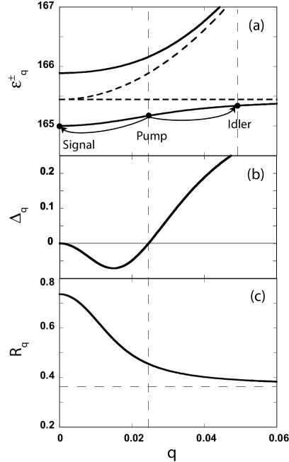
Figure 2: (a) Dispersion $\mathcal{E}^{\pm}_{\mathbf{q}}$ of the lower and upper microcavity polariton branches, as given in eq. (24), for the typical experimental conditions described in the text. The scattering of two pump polaritons at the “magic” angle into a signal polariton at $\mathbf{q}=\mathbf{0}$ and an idler at $2\mathbf{q}$ is also sketched. (b) Detuning $\Delta_{\mathbf{q}}$ associated to this scattering process, as a function of the pump wave vector $\mathbf{q}$. We see that energy is conserved for $q=0.025$, which corresponds to a magic pump angle outside the microcavity $\theta\simeq 15^{\circ}$. (c): Ratio $R_{\mathbf{q}}$ of the photon assisted exchange scattering and the Coulomb scattering, defined in eq. (26) for the transition rate of two polaritons $(\mathbf{q},\mathbf{q})$ scattered into $(\mathbf{0},2\mathbf{q})$. In the figure, the energies are in $e^{2}/\epsilon a_{X}$ unit and the momenta in $a_{X}^{-1}$ unit.

References

- [1] J.J. Hopfield, Phys. Rev. 122, 1555 (1958).
- [2] F. Dubin, M. Combescot and B. Roulet, Europhys. Lett. 69, 931 (2005).
- [3] F. Bassani, F. Ruggiero and A. Quattropani, Il Nuevo Cimento 7, 700 (1986).
- [4] M. Combescot and O. Betbeder-Matibet, Solid State Com. 80, 1011 (1991).
- [5] A. Mysyrowicz, D. Hulin, A. Antonetti, A. Migus, W.T. Masselink and H. Morkoç, Phys. Rev. Lett. 56, 2748 (1986).
- [6] For a review, see M. Combescot, Phys. Rep. 221, 168 (1992).
- [7] M. Combescot, Solid State Com. 74, 291 (1990).
- [8] M. Combescot and O. Betbeder-Matibet, Solid State Com. 134, 11 (2005), and references therein.
- [9] M. Combescot, O. Betbeder-Matibet and R. Combescot, Cond-mat/0702260, to be published in Phys. Rev. B.
- [10] M. Combescot and O. Betbeder-Matibet, Phys. Rev. B 74, 125316 (2006).
- [11] M. Combescot, O. Betbeder-Matibet, K. Cho and H. Ajiki, Europhys. Lett. 72, 618 (2005).
- [12] A. Abrikosov, L. Gorkov, I. Dzyaloshinski, Methods of Quantum Field Theory in Statistical Physics, Prentice-Hall, Englewood Cliffs, N.J. (1963).
- [13] A. Fetter, J. Walecka, Quantum Theory of Many-particle Systems, McGraw-Hill, New York, (1971).
- [14] H. Haug and S. Schmitt-Rink, Prog. Quantum Electron. 9, 3 (1984).
- [15] M. Combescot and O. Betbeder-Matibet, Europhys. Lett. 58, 87 (2002).
- [16] M. Combescot and O. Betbeder-Matibet, Phys. Rev. Lett. 93, 016403 (2004).
- [17] M. Richard, J. Kasprzak, R. Andre, R. Romestain, L.S. Dang, G. Malpuech and A. Kavokin, Phys. Rev. B 72, 201301 (2005).
- [18] J. Kasprzak et al., Nature 443(7110), 409 (2006)
- [19] To get eq. (14), we have used eq. (12) and the fact that is equal to zero, which follows from , the sums over ’s being performed through closure relations.
- [20] G. Rochat, C. Ciuti, V. Savona, C. Piermarocchi and A. Quattropani, Phys. Rev. B 61, 13856 (2000).
- [21] C. Ciuti, P. Schwendimann, B. Deveaud and A. Quattropani, Phys. Rev. B 62, R4825 (2000).
- [22] O. Betbeder-Matibet and M. Combescot, Eur. Phys. J. B 27, 505 (2002).
- [23] P.G. Savvidis et al., Phys. Rev. Lett. 84, 1547 (2000).