Numerical Propagation of Cosmic Rays in the Galaxy

Abstract

We present a Monte-Carlo (MC) calculation of the propagation of cosmic ray protons in the Galaxy for energies above 1 PeV. We discuss the relative strengths of competing effects such as parallel/perpendicular diffusion and drifts in toy models of the Galaxy. We compare our estimates with the results of the MC calculation for the toy models and then we apply the MC calculation to a few more realistic models of the Galactic magnetic field. We study the containment times in different models of the magnetic field in order to understand which one may be consistent with the low energy data.

1 Introduction

The transport of cosmic rays in the Galaxy is usually studied solving the diffusion-convection equation from a distribution of sources in a medium with given diffusion properties. This approach, although very successful (see Ref. [1] for a recent review), can not be applied at arbitrarily high energy because at some point the diffusion approximation breaks down. In the Galaxy this happens, for protons, around $10^{17}\,\mathrm{eV}$. The study of CR transport in this energy region is performed using numerical simulations of the propagation of single particles in the Galactic magnetic field (GMF). Besides the obvious advantage of being able to study the transition region, another advantage of the latter method is the ability to use more realistic models of the GMF, including the arms, all the gradients and so on. The big drawback of this approach is in the computing time that makes it usable only at high energy ($10^{15}\,\mathrm{eV}$ and above).

From observations at low energy, $\sim\,\mathrm{GeV}$, the residence time of particles in the Galaxy is estimated at about $10^{7}\,\mathrm{yr}$ with an energy dependence of $E^{-0.6}$. When extrapolated to higher energies, this trend produces nonsensical results, predicting, for example, huge anisotropies already around $10^{15}\,\mathrm{eV}$ where they are not observed. Assuming an energy dependence of $E^{-1/3}$, as one would expect from Kolmogorov turbulence, the extrapolations are much better, but still a few times larger than the experimental results [2].

In principle one would want to use the diffusion-convection equation at low energy, the numerical simulations at high energy and possibly match the two results in between. Up to now, the simulations at high energy [3] were not successful in this respect. The containment time at $10^{17}\,\mathrm{eV}$ is calculated as $10^{5}\,\mathrm{yr}$ with an energy dependence of $1/E$. Extrapolated to lower energy, this result produces escape times exceeding the age of the universe.

In order to investigate this discrepancy, we developed a numerical simulation of the propagation of particles in arbitrary magnetic fields and we applied it to several toy models of the Galaxy to separately study the various effects contributing to the transport, such as parallel and perpendicular diffusion, drifts and so on. For details on the simulation code see Ref. [4].

2 Diffusion Coefficients

We calculate the diffusion coefficients in a magnetic field composed of a constant regular field in the $z$ direction and a turbulent field with a Kolmogorov spectrum. We inject particles in this field and we follow their trajectories recording their positions as a function of time. Fitting the distribution of the particle positions as a function of time we calculate the diffusion coefficients along the three axes. For the parallel diffusion coefficient we find the usual energy dependence of $E^{1/3}$ at low energy and $E^{2}$ at high energy, whereas for the perpendicular one we find a steeper dependence at low energy: $E^{0.5-0.6}$. This is already an interesting result because it means that in particular geometries where the transport is dominated by perpendicular diffusion one can obtain, from a Kolmogorov spectrum of turbulence, a diffusion coefficient, and therefore a residence time, steeper than the usual one.

3 Toy Models

The first toy model we consider has a purely azimuthal magnetic field that is constant, $1\,\mu\mathrm{G}$, everywhere. Superimposed to this regular field there is a turbulent component whose magnitude is proportional to the one of the regular field with a proportionality constant of $0.5$, $1$ or $2$. We inject particles at the solar system position ($8.5\,\mathrm{kpc}$ from the center) and we record the time required for escaping a cylinder with half-height of $0.5\,\mathrm{kpc}$ and radius of $10\,\mathrm{kpc}$. It is important to note that in this scenario the transport is dominated by the perpendicular diffusion and possibly by drifts, and that the parallel diffusion can be completely neglected since it scatters the particles back and forth along the field lines, but it does not help them escaping the disk since the field lines are closed. The times of escape are plotted with colored points in Fig. 1. The red upward, blue downward triangles and green squares correspond to three different levels of turbulence: $\delta B/B=0.5,1,2$ respectively. The thick solid straight line represents the drift time-scale calculated for the average drift velocity, whereas the thin solid lines are the time-scales for perpendicular diffusion; they are proportional to $h^{2}/D_{\perp}$. The perpendicular diffusion coefficient is the one calculated as described in the previous section. As it is clear from Fig. 1 the transport description as perpendicular diffusion is pretty good for the two cases $\delta B/B=1$ and $2$, but it is not very accurate for $\delta B/B=0.5$. The discrepancy is at low energy, around $10^{15}\,\mathrm{eV}$, and in this region the drift time-scale is much bigger than the diffusion one and then this effect is not caused simply by drifts: they are relevant only at higher energies. The effect is however produced by the curvature of the field lines since injecting the particles at $85\,\mathrm{kpc}$, where the curvature is ten times smaller, produces a time of escape that is in much better accord with the diffusion time-scale (see light blue upward triangles in Fig. 1).

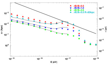
Figure 1: Times of escape in the azimuthal field. The colored points are the results of the simulations for different scenarios. The thin lines are expected escape times calculated with the diffusion coefficient, whereas the thick straight line is the timescale for drifts.

In order to better understand this effect we calculate the diffusion coefficients in the curved magnetic field to check if the curvature of the field lines has an effect also on the diffusion coefficients. Our results are plotted in Fig. 2. We find that with smaller levels of turbulence the two perpendicular diffusion coefficients, in the radial and in the $z$ direction, are modified. The first one is increased and the second one is decreased. This is consistent with the results of Fig. 1, since a smaller diffusion coefficient in the $z$ direction produces a larger time of escape. Reducing the curvature of the field lines, i.e. calculating the diffusion coefficients at larger distances from the center, the effect is reduced (see dotted lines in Fig. 2). The effect promptly disappears increasing the level of turbulence. Fig. 2 is then telling us that the curvature of the field lines not only produces a drift, or the rigid displacement of the distribution of the particle positions, but it also affects the way the distribution evolves with time along the three directions.

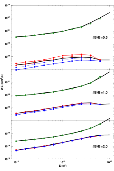
Figure 2: Diffusion coefficients in a curved regular field for the level of turbulence indicated in the plots. In each plot the black lines are the parallel (upper) and perpendicular (lower) diffusion coefficients obtained in the constant field. The green, red and blue lines are diffusion coefficients respectively in the azimuthal, radial and $z$ direction. Solid lines are for injection at $8.5\,\mathrm{kpc}$, dotted lines are for injection at $85\,\mathrm{kpc}$.

Though keeping in mind that this is only a toy model of the magnetic field of the Galaxy, it is interesting to note that at energy $10^{15}\,\mathrm{eV}$ the escape time is $\tau_{15}\approx 0.5-5$ million years (the halo height here is only $0.5\,\mathrm{kpc}$). These numbers are of the same order of magnitude of the confinement times estimated from the abundance of light element in the GeV region, which means that in order to fit these observations one should postulate that the escape time below $10^{15}\,\mathrm{eV}$ should be practically energy independent. We could not envision any realistic mechanism able to justify such an expectation. It follows that within the limitations of the present toy model it is very hard to obtain a realistic, even qualitative, description of what is observed in the Galaxy at much lower energies. This conclusion is confirmed also by the curves on the grammage that show that at $10^{15}\,\mathrm{eV}$ cosmic rays traverse already a column density of $1-2\,\mathrm{g}\,\mathrm{cm}^{-2}$.

We modified the above toy model introducing several complications mimicking the structure of the Galaxy, for example a gradient in radial direction or in the $z$ direction, but the general result did not change much. The slopes of the times of escape remained quite steep, although the absolute values became smaller due to the increase of the drifts.

4 “Realistic” Galactic Magnetic Fields

The knowledge of the magnetic field in our Galaxy is very poor, both for what concerns its regular component and more so for what concerns the turbulent one. Having this in mind we considered a very simple model with the intent not of being very realistic, but just as an example of how the simple picture presented in the previous section becomes suddenly much more complicated. Indeed, following Ref. [5, 6], we considered the BSS model: it includes the spiral arms, has a radial gradient and a gradient in the $z$ direction, but it does not have an halo field, a bar in the center or other complications.

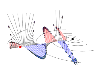
Figure 3: Galactic Magnetic Field and drifts in the BSS models. The black dot is the galactic center, the red one is the solar system position. The black lines show the position of the center of the arms. The blue and red arrows represent the magnitude and direction of the GMF in the given position, while the black arrows show the drift speed.

We plot the drift velocity calculated in several points along the line connecting the galactic center (black dot) with the solar system position (red dot) in Fig. 3. The black lines show the position of the center of the arms, the blue and red arrows represent the magnitude and direction of the GMF in the given position, while the black arrows show the drift speed. In the toy model presented in the previous section the drift velocity was always in the $z$ direction and had a position dependent magnitude. In this case the situation is much more complicated with the drift pushing the particles sometimes toward the center of the arms and sometimes toward the inter-arms space. Moreover in this case both the magnitude and direction of the drift depend on the position and on the pitch angle of the particle. Indeed, in the plot of Fig. 3 the drift velocity is calculated for a particle with an injection cosine with respect to the local magnetic field of $\sqrt{2/3}$ and for a position just above the galactic plane. Calculating it for another pitch angle or another position would produce completely different results. For example, considering the same pitch angle, but a position just below the plane, we would obtain the opposite sign for the radial component of the drift velocity and thus a very different picture.

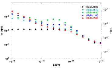
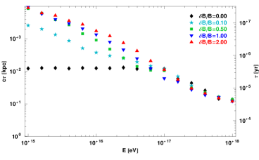
Figure 4: Times of escape in the BSS model for two different ways of normalizing the turbulent component of the field. See text for details.

In Fig. 4 we plot the residence times of protons injected at the solar system position and collected at a cylinder with an half-height of $4\,\mathrm{kpc}$ and a radius of $20\,\mathrm{kpc}$. In each panel we plot several series of points corresponding to different levels of turbulence as indicated. The two panels correspond to two different normalizations of the turbulent component of the field. In the upper panel the $\sqrt{\langle\delta B^{2}\rangle}$ of the turbulent field is in every position a fraction of the regular field. This produces an almost negligible field in the space between the arms, where the regular field switches direction. In the lower plot the magnitude of the turbulent field follows the radial and $z$ dependence of the regular field, except for the arms that are absent in the turbulent component. This means that in this case the ratio $\delta B/B$ is not constant, but variable, being the value indicated in the plot in the center of the arms and going to infinity in the space between the arms.

The times of escape reflect the increased complexity of the model: they are much less regular than the ones obtained in the toy model. The normalization is however of the same order of magnitude with times of escape at $10^{15}\,\mathrm{eV}$ of about $10^{7}\,\mathrm{yr}$ and grammages of a few $\,\mathrm{g}\,\mathrm{cm}^{-2}$. The slopes for the times of escape are $\sim 0.7$ and there is no sign of a possible transition to a flatter slope that would help reconcile these values with the ones measured at low energies.

Acknowledgments. The work of D.D.M. and T.S. is funded in part by NASA APT grant NNG04GK86G. The work of P.B. is partially funded through grant PRIN-2004.

References

- [1] A.W. Strong, I.V. Moskalenko and V.S. Ptuskin, astro-ph/0701517
- [2] A.M. Hillas, Journal of Physics G Nuclear Physics 31 (2005) 95
- [3] V.N. Zirakashvili et al., Astronomy Letters 24 (1998) 139
- [4] D. De Marco, P. Blasi and T. Stanev, arXiv:0705.1972
- [5] J.L. Han and G.J. Qiao, A&A 288 (1994) 759
- [6] T. Stanev, Astrophys. J. 479 (1997) 290