Generation of linear waves in the flow of Bose-Einstein condensate past an obstacle

Abstract

The theory of linear wave structures generated in Bose-Einstein condensate flow past an obstacle is developed. The shape of wave crests and dependence of amplitude on coordinates far enough from the obstacle are calculated. The results are in good agreement with the results of numerical simulations obtained earlier. The theory gives a qualitative description of experiments with Bose-Einstein condensate flow past an obstacle after condensate’s release from a trap.

1 Introduction

After Bose-Einstein condensation of dilute gases was obtained experimentally, great attention has been devoted to excitations existing in such systems (see, e.g., [1]). For example, it is well known that sound waves can propagate through the condensate with repulsive interaction between atoms. Such a condensate can occupy considerable volume inside a trap, therefore, if a wave length is much smaller than the condensate size, one can consider condensate ad locally homogeneous one with a uniform density $n_{0}$ in an undisturbed state. As was shown by Bogoliubov [2], the linear waves have the dispersion law

$$\omega(k)=\sqrt{c_{s}^{2}k^{2}+\left(\frac{\hbar k^{2}}{2m}\right)^{2}},$$ (1)

where

$$c_{s}=\sqrt{\frac{gn_{0}}{m}}$$ (2)

is a speed of sound in a long wave limit $k\to 0$, and $g$ denotes the effective coupling constant

$$g=\frac{4\pi\hbar^{2}a_{s}}{m}$$ (3)

arising due to $s$-wave scattering (with the scattering length $a_{s}$) of atoms with mass $m$. The repulsion of atoms corresponds to $g>0$ and a real speed of sound $c_{s}$. For small wave numbers the dispersion law (1) corresponds to the sound waves propagating with speed $c_{s}$,

$$\omega\cong c_{s}k,\qquad k\to 0,$$ (4)

but for large $k$ it gives the quantum dispersion law of free particles with mass $m$,

$$\omega\cong\frac{\hbar k^{2}}{2m},\qquad k\to\infty.$$ (5)

Transition from one limiting case to another takes place at $k\sim\xi^{-1}$ where $\xi$ is a characteristic parameter called a healing length

$$\xi=\frac{\hbar}{\sqrt{2mgn_{0}}}=\frac{\hbar}{\sqrt{2}mc_{s}}.$$ (6)

If the amplitude is not small and the condensate is not homogeneous, in the mean-field approach dynamics of the condensate is described by the Gross-Pitaevskii equation [1]

$$i\hbar\frac{\partial\psi}{\partial t}=-\frac{\hbar^{2}}{2m}\Delta\psi+V(\mathbf{r})\psi+g|\psi|^{2}\psi,$$ (7)

where $\psi({\bf r})$ is a “condensate wave function”, and $V({\bf r})$ is an external potential (for example, it might be the confining potential of a trap). In the region where condensate is homogeneous, potential $V$ is constant; hence, it can be excluded from the equation by multiplication of $\psi$-function by an inessential phase factor. Linearizing equation (7) with respect to a state with a constant density $n_{0}=|\psi|^{2}$ yields solutions in the form of plane waves with the dispersion law (1). But appearance of the nonlinear term in (7) leads to new kinds of nonlinear excitations—vortices and dark solitons. Linear sound waves of the described origin were observed in the experiment [3] and dark solitons in [4, 5]. If we consider evolution of the condensate with effectively one spatial dimension and the initial disturbance of density is large enough, then the pulse of rarefication will decay into a series of dark solitons [6]. But if the initial disturbance of density is positive, it will lead to wave breaking of the pulse with formation of the dispersive shock wave [7, 8], as it has been found experimentally in [9, 10].

Linear waves, dark solitons and shock waves referred above can be described in the first approximation as waves depending only on time and one space coordinate. But situation becomes completely different if the wave behavior depends on two space coordinates. In particular, the experiment [11] (see also [12]) has been made where condensate released from a trap interacted during its expansion with a small obstacle generated by a laser beam. As was shown experimentally, the flow past an obstacle generates wave structures in the form of stationary “moustaches” attached to the obstacle. Theoretical analysis [13, 14] shows that the wave structure generated in the flow can be subdivided into two regions separated by the Mach cone corresponding to the sound velocity $c_{s}$ in the long wave limit, i.e. by lines drawn at the angle $\theta$ to the direction of the flow so that

$$\sin\theta=\frac{c_{s}}{u_{0}}=\frac{1}{M},$$ (8)

where $M$ is the Mach number. As was shown in [13, 14], inside the Mach cone dark solitons are generated. Their slope depends on their depth—the most shallow solitons lie near the Mach cone and the deepest ones are located near the flow axis going through the obstacle. In the paper [13] the exact stationary solution of the Gross-Pitaevskii equation was found and it was shown by numerical calculation that this solution describes dark solitons generated inside the Mach cone. Linear waves are characterized by the dispersion law (1), where $k$ means the module of the wave number. This dispersion law shows that both phase and group velocities are greater than the sound velocity $c_{s}$ in a long wavelength limit. It means that linear wave structure formed by a wave packet can only occupy the region outside the Mach cone defined by the equation (8). For the first time these waves described by the Gross-Pitaevskii equation were observed in the numerical experiment [15]. In the paper [12] analogous numerical simulation was carried out for description of the structures observed in the experiments with the condensate flow past obstacle. Some of the elementary characteristics of these structures were derived from the dispersion law (1). In the paper [16] it was noticed that these waves have a physical origin analogous to Kelvin’s ship waves [17] generated by a ship moving in a still water. It means that similar computation methods [18, 19] can be used in the case of Bose-Einstein condensate. In [16] such a theory was developed and shape of waves crests was obtained. It was shown that this theory agrees very well with numerical simulations. But it cannot give the dependence of the wave amplitudes on space coordinates. The aim of this paper is to develop a complete theory which can give not only geometrical but also dynamical properties of the wave structures generated outside the Mach cone by the condensate flow past obstacle.

2 The theory of stationary wave structures generated by condensate flow past obstacle

As a basis of the theory, we take Kelvin’s method in the form presented in [18]. According to this theory, the wave structures result from interference of linear waves emitted by the source at all previous moments of time. We take a source (obstacle) at rest, in agreement with the experiment [11], and suppose that condensate moves with a constant speed $u_{0}$ in the direction of the $x$ axis. Since a stationary flow corresponds to the potential $V({\bf r})$ turned on in the infinite past, one can consider this physical condition by the assumption that the potential rises in time according to the law $V({\bf r},t)=\exp(\varepsilon t)V({\bf r})$. Afterwards one should take the limit $\varepsilon\longrightarrow 0$.

It is convenient to transform the Gross-Pitaevskii equation $\psi({\bf r},t)$ to a “hydrodynamic” form by means of the substitution

$$\psi({\bf r},t)=\sqrt{n({\bf r},t)}\exp\left(\frac{i}{\hbar}\int^{{\bf r}}{{\bf U}}({\bf r}^{\prime},t)d{\bf r}^{\prime}\right),$$ (9)

where $n({\bf r},t)$ is a local density of atoms in condensate, ${{\bf U}}({\bf r},t)$ is a velocity field of condensate flow. To simplify the notation, let us introduce non-dimensional variables

$$\tilde{{\bf r}}=\frac{{\bf r}}{\sqrt{2}\xi},\quad\tilde{t}=\frac{c_{s}}{\sqrt{2}\xi}t,\quad\tilde{n}=\frac{n}{n_{0}},\quad\tilde{{\bf U}}=\frac{{\bf U}}{c_{s}},$$ (10)

and dimensionless potential of the obstacle

$$\tilde{V}({\bf r})=\frac{1}{mc_{s}^{2}}V(\sqrt{2}\,\xi\tilde{{\bf r}}).$$ (11)

where $n_{0}$ is a density of undisturbed condensate (infinitely far from the obstacle). Upon substitution of (9), (10) and (11) into (7) and separation of real and imaginary parts, we obtain equations for the condensate density $n$ and velocity components ${\bf U}=(u(x,y,t),v(x,y,t))$ in a hydrodynamic form:

$$\begin{split}n_{t}+(nu)_{x}+(nv)_{y}&=0,\\ u_{t}+uu_{x}+vu_{y}+n_{x}+\left(\frac{n_{x}^{2}+n_{y}^{2}}{8n^{2}}-\frac{n_{xx}+n_{yy}}{4n}\right)_{x}&=-V_{x}e^{\varepsilon t},\\ v_{t}+uv_{x}+vv_{y}+n_{y}+\left(\frac{n_{x}^{2}+n_{y}^{2}}{8n^{2}}-\frac{n_{xx}+n_{yy}}{4n}\right)_{y}&=-V_{y}e^{\varepsilon t},\end{split}$$ (12)

where tildes are omitted for convenience of the notation and the indices stand for derivatives with respect to appropriate variables.

We are interested in linear waves propagating in a uniform flow with $n_{0}=1$, $u_{0}=M$, $v_{0}=0$. Therefore we introduce new variables

$$n=1+n_{1},\quad u=M+u_{1},\quad v=v_{1}$$ (13)

and linearize the system (12) with respect to small deviations $n_{1},\,u_{1},\,v_{1}$ from a uniform flow. As a result we arrive at a linear system

$$\begin{split}n_{1,t}+u_{1,x}+Mn_{1,x}+v_{1,y}&=0,\\ u_{1,t}+Mu_{1,x}+n_{1,x}-\tfrac{1}{4}(n_{1,xxx}+n_{1,xyy})&=-V_{x}e^{\varepsilon t},\\ v_{1,t}+Mv_{1,x}+n_{1,y}-\tfrac{1}{4}(n_{1,xxy}+n_{1,yyy})&=-V_{y}e^{\varepsilon t}.\end{split}$$ (14)

A stationary solution corresponds to the limit $\varepsilon\to 0$, where all the variables depend on time as $\exp(\varepsilon t)$. Fourier transform for spatial variables yields the solution

$${}n_{1}=-e^{\varepsilon t}\int\!\!\int\frac{k^{2}\Phi(k_{x},k_{y})e^{i(k_{x}x+k_{y}y)}}{(\varepsilon+ik_{x}M)^{2}+k^{2}(1+{k^{2}}/{4})}\frac{dk_{x}dk_{y}}{(2\pi)^{2}},$$ (15)

where

$$\Phi({\bf k})=\int V({\bf r})e^{-i{\bf k}{\bf r}}d{\bf r}.$$ (16)

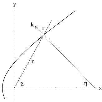
Figure 1: Polar coordinates defining the radius vector ${\bf r}$ and the wave vector ${\bf k}$ normal to the wave front which is shown schematically by a curved line.

Far enough from the obstacle its potential can be considered as a point-like one, $V({\bf r})=V_{0}\delta({\bf r})$; hence we have $\Phi({\bf k})=V_{0}$. It is convenient to introduce polar coordinates (see Fig. 1) for vectors ${\bf r}$ and ${\bf k}$:

$$x=r\cos{\chi},\quad y=r\sin{\chi};\qquad k_{x}=-k\cos{\eta},\quad k_{y}=k\sin{\eta}.$$ (17)

Then simple transformation of equation (15) gives

$$n_{1}=\frac{V_{0}}{\pi^{2}}\,e^{\varepsilon t}\int_{-\pi}^{\pi}\int_{0}^{\infty}\frac{ke^{-ikr\cos(\chi+\eta)}dkd\eta}{k^{2}-k_{0}^{2}-i\delta\cos{\eta}},$$ (18)

where $\delta={8M\varepsilon}/k$ is a small positive quantity and

$$k_{0}=2\sqrt{M^{2}\cos^{2}{\eta}-1}.$$ (19)

One can divide the integration interval over $\eta$ into two parts: $\int d\eta=\int_{-\pi/2}^{\pi/2}d\eta+\int_{\pi/2}^{3\pi/2}d\eta$. After replacement $\eta^{\prime}=\eta-\pi$ in the second integral, one can notice that the integrand function converts to its complex conjugate one. Hence we can write the integral (18) in the form

$$n_{1}=\frac{2V_{0}}{\pi^{2}}e^{\varepsilon t}\mathrm{Re}\int_{-\pi/2}^{\pi/2}\int_{0}^{\infty}\frac{ke^{-ikr\cos(\chi+\eta)}dkd\eta}{k^{2}-k_{0}^{2}-i\delta\cos{\eta}}.$$ (20)

Integration over $k$ should be taken along the positive axis. The pole

$$k=\sqrt{k_{0}^{2}+i\delta\cos\eta}\cong k_{0}+i\frac{\delta\cos\eta}{2k_{0}},$$ (21)

lies in vicinity of a real axis, so we can expect that it gives the main contribution into the integral. This can be proved by the following argumentation. We add to the integration contour along real positive $k$ axis also integration along the positive or negative imaginary axis and a quarter of a circle with infinite radius to make the contour closed. If $\cos(\chi+\eta)<0$, we use contour along the boundary of the first quadrant of complex $k$–plane, on the other hand, if $\cos(\chi+\eta)>0$, we use the contour along the boundary of the fourth quadrant. In both cases integration along a quarter of a circle vanishes when radius $|k|$ of the circle tends to infinity. Thus, we have no contribution of this part of the integration contour. The pole (21) gets inside the integration contour only if one take the integral along the boundary of the first quadrant what corresponds to the case $\cos(\chi+\eta)<0$. In this case the result of integration along the real positive axis $k$ is equal to contribution of the residue and integration along the positive imaginary axis. If we have $\cos(\chi+\eta)>0$, this integral is equal to the integral along the negative imaginary axis only. In both cases an estimation of integral along the imaginary axis gives

$$\int_{0}^{\infty}\frac{ke^{-kr\cos(\chi+\eta)}dk}{k^{2}+k_{0}^{2}}\propto\frac{1}{r^{2}},$$ (22)

which means that this contribution decreases as $r^{-2}$ with distance $r$ from the obstacle. As we shall see below, the contribution of the pole decreases as $r^{-1/2}$. It means that far enough from the obstacle we can neglect the contribution of integration along the imaginary axis. Thus, a noticeable wave structure appears in the region where $\cos(\chi+\eta)<0$, i.e. the angle $\mu=\pi-(\chi+\eta)$ between vectors ${\bf r}$ and ${\bf k}$ should be acute. The contribution of the pole (21) is equal to

$$n_{1}=-\frac{2V_{0}}{\pi}\,\mathrm{Im}\int_{-\pi/2}^{\pi/2}e^{-ikr\cos(\chi+\eta)}d\eta,$$ (23)

where $k$ is determined by the equation (19) (index “0” is dropped here).

Far from the obstacle where the phase ${\bf k}{\bf r}=rs$ is large enough, we have large values of

$$s(\eta)=k(\eta)\cos(\chi+\eta),$$ (24)

and integral (23) can be estimated by a standard method of stationary phase. Condition $\partial s/\partial\eta=0$ gives the equation for the point of stationary phase and it can be easily transformed to the form

$$\tan\mu=\frac{2M^{2}}{k^{2}}\sin 2\eta$$ (25)

or, with the help of equation for $\mu$, it gives the expression for $\chi$,

$$\tan\chi=\frac{(1+k^{2}/2)\tan\eta}{M^{2}-(1+k^{2}/2)}.$$ (26)

Taking into account equation (19), we find

$$\cos{\mu}=\frac{k^{2}}{2[(M^{2}-2)k^{2}+4(M^{2}-1)]^{1/2}}.$$ (27)

With account of (25), we get the expression for a second derivative of the phase

$$\frac{\partial^{2}s}{\partial\eta^{2}}=8\frac{\cos{\mu}}{k^{3}}[(M^{2}-2)k^{2}+6(M^{2}-1)].$$ (28)

As a result, the expression for the condensate density (23) takes the form

$$n_{1}=V_{0}\sqrt{\frac{2k}{\pi r}}\frac{[(M^{2}-2)k^{2}+4(M^{2}-1)]^{1/4}}{[(M^{2}-2)k^{2}+6(M^{2}-1)]^{1/2}}\cos\left(kr\cos{\mu}-\frac{\pi}{4}\right).$$ (29)

First of all, let us check that the results obtained above agree with the theory developed in [16]. Since the wave crest corresponds to the constant value of the phase $\phi=kr\cos\mu,$ we can find the equation for the absolute value of the radius-vector

$$r=\frac{\phi}{k\cos\mu}=\frac{2\phi}{k^{3}}[(M^{2}-2)k^{2}+4(M^{2}-1)]^{1/2}.$$ (30)

Calculating $\cos\chi$ and $\sin\chi$ with the help of equation (26), we obtain equations for lines of stationary phase coinciding with those found by another method in [16]:

$$\begin{split}&x=r\cos\chi=\frac{4\phi}{k^{3}}\cos\eta(1-M^{2}\cos 2\eta),\\ &y=r\sin\chi=\frac{4\phi}{k^{3}}\sin\eta(2M^{2}\cos^{2}\eta-1).\end{split}$$ (31)

Since the wave vector $k$ is determined as a function of $\eta$ by equation (19), equations (31) give the wave crests shape in a parametric form where parameter $\eta$ varies in the interval

$$-\arccos(1/M)\leq\eta\leq\arccos(1/M).$$ (32)

For small $\eta$ we have

$$\begin{split}&x\cong-\frac{\phi}{2\sqrt{M^{2}-1}}+\frac{(2M^{2}-1)\phi}{4(M^{2}-1)^{3/2}}\eta^{2},\\ &y\cong\frac{(2M^{2}-1)\phi}{2(M^{2}-1)^{3/2}}\eta,\end{split}$$ (33)

that is the lines of stationary phase take here a parabolic form

$$x(y)\cong-\frac{\phi}{2\sqrt{M^{2}-1}}+\frac{(M^{2}-1)^{3/2}}{(2M^{2}-1)\phi}y^{2}.$$ (34)

The limiting values $\eta=\pm\arccos{(1/M)}$ correspond to the lines

$$\frac{x}{y}=\pm\sqrt{M^{2}-1},$$ (35)

i.e. far from the obstacle wave crest curves approach to the straight lines parallel to those forming the Mach cone (8).

An example of the wave structure determined by equation (29) with $M=4$ is shown on Fig. 2.

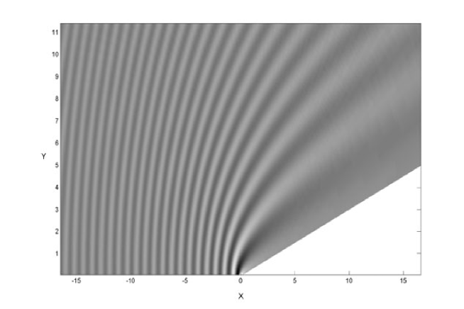
Figure 2: Wave structure calculated according to equation (29) with $M=4$; it is generated outside the Mach cone and only its upper part with $y>0$ is shown.

If $M\gg 1$, there exists a region where $M\cos\eta\gg 1$; all the equations get here a simple form. In particular, we have $\chi\cong\pi-2\eta$, $\mu\cong\eta\cong({\pi}-{\chi})/2$, so that

$$k\cong 2M\sin{\frac{\chi}{2}}\gg 1$$ (36)

and as a result the expression for condensate density (29) takes the form

$$n_{1}\cong V_{0}\sqrt{\frac{2}{\pi Mr}}\cos\left(2Mr\sin^{2}{\frac{\chi}{2}}-\frac{\pi}{4}\right).$$ (37)

The expressions (31) take here a parabolic form

$$x=-\frac{\phi}{2M}+\frac{M}{2\phi}y^{2},$$ (38)

Naturally, this result can be obtained from (32) in the limiting case $M\gg 1$.

In the region in front of the obstacle where $y=0,\,x<0$, the perturbations of the condensate density take the simplest form. Here we have

$$k=2\sqrt{M^{2}-1},$$ (39)

i.e. the wave length $\lambda=2\pi/k$ is constant and

$$n_{1}=2V_{0}\sqrt{\frac{(M^{2}-1)^{1/2}}{\pi(2M^{2}+1)r}}\cos\left[-2\sqrt{M^{2}-1}\,x-\frac{\pi}{4}\right],\quad y=0,\quad x<0.$$ (40)

The plot illustrating this dependence is shown in Fig. 3. All the results obtained above are in a good agreement with a numerical simulations carried out in [16].

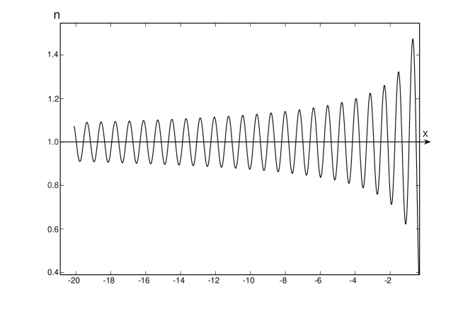
Figure 3: Oscillations of the condensate density in a stationary wave in front of the obstacle: $x<0$, $y=0$. The condensate flow corresponds to the Mach number $M=4$.

3 Conclusions

The theory developed here is valid as long as the amplitude of the wave structure is much smaller than unity (in dimensionless variables), i.e.

$$r\gg V_{0}^{2}/M.$$ (41)

Far enough from the obstacle this condition is always fulfilled. But for comparison of our theory with experiment it is also necessary that the condensate flow be uniform in the region under consideration. The estimates made in [13] show that one can satisfy this condition for a free flow of condensate released from the trap by locating the obstacle far enough from the center of the trap and sufficiently long time after condensate’s release. As far as we can see, this conditions were not fulfilled in the experiment [11, 12]. In particular, the obstacle was situated too close to the center of the flow and its size was too large, so that the shadow region appeared behind it which was not filled by the condensate. We believe that for this reason no dark solitons predicted in [13] were observed experimentally. Nevertheless the wave structure in [11, 12] looks similar to one shown in Fig. 2. Thus we believe that the theory developed above gives at least qualitative description of the wave structures observed experimentally.

Acknowledgements

We are grateful to G.A. El and A. Gammal for useful discussions. This work was supported by RFBR (grant 05-02-17351).

References

- [1] L.P. Pitaevskii and S. Stringari, Bose-Einstein Condensation, Cambridge University Press, Cambridge, 2003.
- [2] N.N. Bogoliubov, Izv. Acad. Nauk USSR, ser. fiz. 11, 77 (1947).
- [3] M.R. Andrews, D.M. Kurn, H.-J. Miesner, D.S. Durfee, C.G. Townsend, S. Innouye, W. Ketterle, Phys. Rev. Lett. 79, 553 (1997); 80, 2967(E) (1998).
- [4] S. Burger, K. Bongs, S. Dettmer, W. Ertmer, K. Sengstock, A. Sanpera, G.V. Shlyapnikov, and M. Lewenstein, Phys. Rev. Lett. 83, 5198 (1999).
- [5] J. Denschlag, J.E. Simsarian, D.L. Feder, C.W. Clark, L.A. Collins, J. Cubizolles, L. Deng, E.W. Hagley, K. Helmerson, W.P. Reinhart, S.L. Rolston, B.I. Schneider, and W.D. Phillips, Science 287, 97 (2000).
- [6] V.A. Brazhnyi, A.M. Kamchatnov, Phys. Rev. A 68, 043614 (2003).
- [7] A.M. Kamchatnov, A. Gammal, R.A. Kraenkel, Phys. Rev. A 69, 063605 (2004).
- [8] B. Damski, Phys. Rev. A 69, 043610 (2004).
- [9] T.P. Simula, P. Engels, I. Coddington, V. Schweikhard, E.A. Cornell, R.J. Ballagh, Phys. Rev. Lett. 94, 080404 (2005).
- [10] M.A. Hoefer, M.J. Ablowitz, I. Coddington, E.A. Cornell, P. Engels, V. Schweikhard, Phys. Rev. A 74, 023623 (2006).
- [11] E.A. Cornell, “Conference on Nonlinear Waves, Integrable Systems and their Applications”, (Colorado Springs, June 2005); http://jilawww.colorado.edu/bec/papers.html.
- [12] I. Carusotto, S.X. Hu, L.A. Collins, and A. Smerzi, Phys. Rev. Lett. 97, 260403 (2006).
- [13] G.A. El, A. Gammal, and A.M. Kamchatnov, Phys. Rev. Lett. 97, 180405 (2006).
- [14] G.A. El, Yu.G. Gladush, and A.M. Kamchatnov, J. Phys. A: Math. Theor. 40, 611 (2007).
- [15] T. Winiecki, J.F. McCann, and C.S. Adams, Phys. Rev. Lett. 82, 5186 (1999).
- [16] Yu.G. Gladush, G.A. El, A. Gammal, and A.M. Kamchatnov, Phys. Rev. A 75, 033619 (2007).
- [17] Lord Kelvin, Phil. Mag. 9, 733 (1905).
- [18] G.B. Whitham, Linear and nonlinear waves, Wiley-Interscience (1974).
- [19] R.S. Johnson, A Modern Introduction to the Mathematical Theory of Water Waves, Cambridge University Press, Cambridge, (1997).