Exact Solutions of Semiclassical Non-characteristic Cauchy Problems for the Sine-Gordon Equation

Abstract.

The use of the sine-Gordon equation as a model of magnetic flux propagation in Josephson junctions motivates studying the initial-value problem for this equation in the semiclassical limit in which the dispersion parameter $\varepsilon$ tends to zero. Assuming natural initial data having the profile of a moving $-2\pi$ kink at time zero, we analytically calculate the scattering data of this completely integrable Cauchy problem for all $\varepsilon>0$ sufficiently small, and further we invert the scattering transform to calculate the solution for a sequence of arbitrarily small $\varepsilon$. This sequence of exact solutions is analogous to that of the well-known $N$-soliton (or higher-order soliton) solutions of the focusing nonlinear Schrödinger equation. Plots of exact solutions for small $\varepsilon$ reveal certain features that emerge in the semiclassical limit. For example, in the limit $\epsilon\rightarrow 0$ one observes the appearance of nonlinear caustics, i.e. curves in space-time that are independent of $\varepsilon$ but vary with the initial data and that separate regions in which the solution is expected to have different numbers of nonlinear phases.

In the appendices we give a self contained account of the Cauchy problem from the perspectives of both inverse scattering and classical analysis (Picard iteration). Specifically, Appendix A contains a complete formulation of the inverse-scattering method for generic $L^{1}$-Sobolev initial data, and Appendix B establishes the well-posedness for $L^{p}$-Sobolev initial data (which in particular completely justifies the inverse-scattering analysis in Appendix A).

1. Introduction

The sine-Gordon equation

(1) $$\varepsilon^{2}u_{tt}-\varepsilon^{2}u_{xx}+\sin(u)=0$$

describes a broad array of physical and mathematical phenomena. The partial differential equation (1) may be regarded as the continuum limit of a chain of pendula subject to an external (gravity) force and coupled to their nearest neighbors via Hooke’s law. In nonlinear optics, the sine-Gordon equation is a special case of the Maxwell-Bloch equations and describes self-induced transparency in the sharp-line limit [16]. In biology, the sine-Gordon equation models transcription and denaturation in DNA molecules [18]. Bäcklund showed a correspondence between solutions of the sine-Gordon equation and surfaces of constant negative curvature [9].

In solid-state physics, the sine-Gordon equation models idealized magnetic flux propagation along the insulating barrier between two superconductors in a Josephson junction. Here the length $\ell_{0}$ of the transmission line corresponds to a length of $1$ in terms of the dimensionless coordinate $x$ measuring distance along the junction. Let $L$ be the inductance per unit length and $C$ be the capacitance per unit length. Then $v:=(LC)^{-1/2}$ is the typical velocity parameter, and the macroscopic time scale $t$ measures one dimensionless unit when $\ell_{0}/v$ seconds have passed. The parameter $\varepsilon$ is the ratio of the Josephson length $\ell_{J}$ to the transmission line length $\ell_{0}$. The Josephson length $\ell_{J}$ is in turn proportional to $\Phi_{0}^{1/2}$, where $\Phi_{0}:=h/(2\varepsilon)\approx 2.064\times 10^{-15}$ V sec is the quantum unit of magnetic flux. Laboratory experiments by Scott, Chu, and Reible [20] analyzed flux propagation in Josephson junctions of length $\ell_{0}=35$ cm for which $\ell_{J}$ was approximately $10^{-4}$ to $10^{-3}$ m. Therefore, in these experiments, $\varepsilon:=\ell_{J}/\ell_{0}\approx 0.0005$. The period of a signal input to the transmission line in these experiments was typically on the order of $10^{-9}$ seconds, which is approximately one dimensionless time unit on the $t$-scale. Together with $\varepsilon$ being small, this motivates the study of the semiclassical (or zero-dispersion) limit as $\varepsilon\downarrow 0$. For analytical convenience we choose to study the Cauchy initial-value problem on the real line $x\in\mathbb{R}$. Formulating a semiclassical Cauchy problem means fixing functions $f$ and $g$ independent of $\varepsilon$, and then, for all $\varepsilon>0$ sufficiently small, posing the Cauchy problem for (1) with initial data of the form $u(x,0;\varepsilon)=f(x)$, $\varepsilon u_{t}(x,0;\varepsilon)=g(x)$. See Appendix B for an account of the well-posedness theory of this Cauchy problem for $\varepsilon>0$ fixed. Solving the semiclassical Cauchy problem means obtaining the one-parameter family of solutions $u(x,t;\varepsilon)$. We are usually most interested in the asymptotic behavior of the solution as $\varepsilon\downarrow 0$.

In this paper, we consider the sine-Gordon equation (1) for all $\varepsilon>0$ sufficiently small with the initial condition

(2) $$\sin\left(\frac{f}{2}\right):=\text{sech}(x),\quad\cos\left(\frac{f}{2}\right):=\tanh(x),\quad g:=2\mu\,\text{sech}(x),\quad x\in\mathbb{R}$$

where $\mu\in\mathbb{R}$ is a parameter. We refer to the solution of the Cauchy problem as $u(x,t;\varepsilon,\mu)$. The topological charge (or winding number) of solutions satisfying (2) is a constant of motion given by

(3) $$w[u]:=\frac{1}{2\pi}\int_{-\infty}^{+\infty}u_{x}\,dx=-1.$$

From one point of view, the initial data (2) are natural to study, because $u(x,t;\sqrt{\mu^{2}+1},\mu)$ is an exact mathematical antikink solution of the sine-Gordon equation explicitly given by

(4) $$\begin{split}\cos(u(x,t;\sqrt{\mu^{2}+1},\mu))&=1-2\,\text{sech}^{2}\left(\frac{1}{\varepsilon w}(x-vt)\right),\\ \sin(u(x,t;\sqrt{\mu^{2}+1},\mu))&=2\,\text{sech}\left(\frac{1}{\varepsilon w}(x-vt)\right)\tanh\left(\frac{1}{\varepsilon w}(x-vt)\right)\end{split}$$

with velocity $v$ and width parameter $w$ given by

(5) $$v=\frac{1}{\mu^{2}+1-\mu\sqrt{\mu^{2}+1}}-1,\quad w=-\frac{1}{2}\sqrt{1-v^{2}}.$$

From these formulae we see that $u$ is a traveling wave with velocity $v$ bounded by 1 (the light speed), demonstrating the hyperbolicity of the sine-Gordon equation. This solution admits a natural relativistic interpretation since the relationship between $v$ and $w$ corresponds to Lorentz contraction in special relativity.

For $\varepsilon\neq\sqrt{\mu^{2}+1}$, the initial data (2) no longer corresponds to simply one soliton, but in general excites a nonlinear superposition of kinks, antikinks, breathers, and radiation. It is interesting to observe that the initial data (2) satisfies the advection equation $u_{t}+vu_{x}=0$ with constant velocity $v=\mu/\varepsilon$. In this sense, we may consider the initial data as being in uniform motion to the right with velocity $v$. Note, however, that if $\mu\neq 0$, then for $\varepsilon>0$ sufficiently small, the velocity $v$ of the initial data exceeds the constraint $|v|\leq 1$ imposed by the hyperbolic nature of the sine-Gordon equation (1). In this situation, one might expect the sine-Gordon equation to regularize the superluminal velocity of the initial data for $t>0$ by some kind of catastrophic effect that destroys the profile of the initial data. In fact, we will show (see figures 6 and 8) that the regularization of the velocity takes place via the emission of a large number (inversely proportional to $\varepsilon$) of kink-antikink pairs.

The family of solutions corresponding to the initial data (2) may be viewed as an analogue for the sine-Gordon equation of the $N$-soliton (or higher-order soliton) solution to the cubic focusing nonlinear Schrödinger (NLS) equation

(6) $$iq_{t}+\frac{1}{2}q_{xx}+|q|^{2}q=0\,.$$

Satsuma and Yajima [19] found that with initial data $q(x,0;N)$=$N\,\text{sech}(x)$ the scattering data relevant for the focusing NLS equation can be found in closed form for any $N\in\mathbb{R}$. Furthermore, if $N\in\mathbb{Z}$ then the scattering data are reflectionless and so the solution $q(x,t;N)$ can be found more-or-less explicitly. In [17] it was noted that, with $\varepsilon=c/N$ and $\tau=Nt/c$, the function $\phi(x,\tau;\varepsilon)=cq(x,t;N)/N$ satisfies the initial-value problem

(7) $$i\varepsilon\phi_{\tau}+\frac{\varepsilon^{2}}{2}\phi_{xx}+|\phi|^{2}\phi=0,\quad\phi(x,0;\varepsilon)=c\,\text{sech}(x).$$

The functions $\phi(x,\tau;\varepsilon)$ therefore solve a semiclassical Cauchy problem since $\phi(x,0;\varepsilon)$ is independent of $\varepsilon$. Numerical reconstruction of the inverse-scattering solution for $\varepsilon=\varepsilon_{N}=c/N$, $N=1,2,3,\dots$ in [17] revealed a spatio-temporal pattern for $\phi$ emerging as $\varepsilon\downarrow 0$ consisting of a fixed macrostructure with nonlinear caustics (phase transition boundaries or breaking curves) separating regions of the space-time plane consisting of oscillations of different local genus (number of nonlinear phases). At least two caustic curves appear in the dynamics (a primary caustic $t=t_{1}(x)$ and a secondary caustic $t=t_{2}(x)>t_{1}(x)$). The semiclassical asymptotics for times $t$ up to and just beyond the primary caustic were obtained in [12] and these results were extended to times $t$ just beyond the secondary caustic (requiring a substantial modification of the method that captures the primary caustic) in [15]. In a related result, Tovbis and Venakides [21] generalized the calculation of Satsuma and Yajima by computing the scattering data associated with the semiclassically-scaled focusing NLS equation (7) explicitly for all sufficiently small $\varepsilon>0$ when the initial data is given in the form

(8) $$\phi(x,0;\mu)=A(x)e^{iS(x)/\varepsilon},\quad S^{\prime}(x)=-\mu\tanh(x),\,\,A=c\,\text{sech}(x)\,.$$

Subsequently, the Cauchy problem for (7) with this initial data has been studied by Tovbis, Venakides, and Zhou [22, 23]. In this paper, we present a calculation of the scattering data for (1)–(2) analogous to the work in [19] and [21], and we also present an explicit computation of $u(x,t;\varepsilon,\mu)$ as $\varepsilon\downarrow 0$ analogous to [17]. The asymptotic analysis of the semiclassical Cauchy problem for sine-Gordon corresponding to the work in [12, 15, 22, 23] will be carried out in a later work.

The sine-Gordon equation (1) is an integrable system, possessing a Lax pair (see (123) and (124)) and admitting all the benefits thereof, including the existence of inverse-scattering transforms for solving Cauchy problems in various coordinate systems. We consider the Cauchy problem in laboratory coordinates and we use the Riemann-Hilbert formulation of inverse scattering. For the sine-Gordon equation in characteristic coordinates, the inverse-scattering method was first given in [1] and [25]. The inverse-scattering method corresponding to the (noncharacteristic) Cauchy problem for the sine-Gordon equation in laboratory coordinates was worked out by Kaup [13]. An account of the Riemann-Hilbert method for carrying out the inverse step in laboratory coordinates can be found in the text of Faddeev and Takhtajan [8], and further developments to the theory were made by Zhou [26] and Cheng et al. [4]. In our paper, we add to this literature by giving in Appendix A a complete description of the Riemann-Hilbert formulation of the solution of the Cauchy problem in laboratory coordinates assuming that at each instant of time the solution $u$ has $L^{1}$-Sobolev regularity. That the sine-Gordon equation (1) preserves this degree of regularity if it is present at $t=0$ is established by independent arguments in Appendix B.

Briefly, the inverse-scattering method proceeds as follows. Cauchy data for the sine-Gordon equation characterize a set of scattering data, which consist of the reflection coefficient $\rho:\mathbb{R}\rightarrow\mathbb{C}$, the eigenvalues $\{z_{n}\}$, and the modified proportionality constants $\{c_{n}\}$. The scattering data are used to formulate a Riemann-Hilbert problem with an explicit, elementary dependence on $x$ and $t$. While it is not in general possible to solve a Riemann-Hilbert problem in closed form, for reflectionless Cauchy data (i.e. for which $\rho(z)\equiv 0$) the Riemann-Hilbert problem can be reduced to the solution of a system of linear algebraic equations.

In Section 2, we explicitly calculate the scattering data corresponding to viewing the initial data (2) as a kind of potential in the linear scattering problem (123) associated with the Cauchy problem for the sine-Gordon equation (1). Our analysis will be valid for all $\mu\in\mathbb{R}$ and $\varepsilon>0$ sufficiently small. Furthermore, we show that if $\varepsilon$ lies in the sequence

(9) $$\varepsilon=\varepsilon_{N}(\mu):=\frac{\sqrt{\mu^{2}+1}}{2N+1}\,,\quad\quad N\in\mathbb{Z}^{+}:=\{0,1,2,\dots\}$$

(note that this sequence converges to zero as $N\rightarrow\infty$), then the scattering data are reflectionless ultimately implying via inverse-scattering theory that $u$ can be computed explicitly (that is, $u$ can be expressed by a finite number of arithmetic operations). The inverse step is carried out for $\varepsilon$ in the sequence (9) corresponding to reflectionless initial data in Section 3, where $\cos(u)$ and $\sin(u)$ are extracted by considering an appropriate limit of the solution to the Riemann-Hilbert problem. As $\varepsilon\downarrow 0$ through this sequence, a pattern emerges in which $u$ consists of modulated wave trains of wave number and frequency inversely proportional to $\varepsilon$ with one or more nonlinear phases. The spatio-temporal scale of the modulation is fixed as $\varepsilon\downarrow 0$. Regions of space-time containing waves with different numbers of nonlinear phases are separated by nonlinear caustics that are independent of $\varepsilon$ for fixed $\mu$. See figures 5, 6, and 8 for plots of $\cos(u)$ exhibiting these features for various values of $\varepsilon$ and $\mu$. At a qualitative level, these features resemble those observed for solutions of the semiclassical Cauchy problem for the focusing NLS equation. Section 4 discusses the limitations inherent in an approach to the semiclassical limit based upon calculations of complexity and sensitivity increasing with $N\sim\varepsilon^{-1}$, and explores possible extensions.

Remark 1. Under the scalings $x=\varepsilon X$ and $t=\varepsilon T$ and the choice $\varepsilon=\varepsilon_{N}(\mu)$ (see (9)), equations (1) and (2) become

(10) $$U_{TT}-{U}_{XX}+\sin(U)=0,$$

(11) $$\begin{split}\sin\left(\frac{1}{2}U(X,0;N,\mu)\right)=\text{sech}\left(\varepsilon_{N}(\mu)X\right),\quad&\cos\left(\frac{1}{2}U(X,0;N,\mu)\right)=\tanh\left(\varepsilon_{N}(\mu)X\right),\\ U_{T}(X,0;N,\mu)=2\mu\,\text{sech}&\left(\varepsilon_{N}(\mu)X\right),\end{split}$$

where $U(X,T;N,\mu)=u(x,t;\varepsilon,\mu)$. This is a fixed-dispersion Cauchy problem with a sequence of different initial conditions depending on $N$, just as in the problem for the NLS equation studied by Satsuma and Yajima. The initial conditions all have topological charge $w[U]=-1$ but $U(X,0;N,\mu)$ and $U_{T}(X,0;N,\mu)$ become more dilated in $X$ (slowly-varying) as $N$ increases. Therefore, an alternate way of viewing our result is that we can find exact solutions to the fixed-dispersion initial-value problem (10)–(11) for $N\in\mathbb{Z}^{+}$. As an example of an explicit solution of (10) obtained in this way, when $N=1$ and $\mu=0$ we have

(12) $$\cos(U(X,T;1,0))=1-\frac{2n(X,T)^{2}}{d(X,T)^{2}}\,,$$

where

(13) $$\begin{split}n(X,T)&:=11+\cos\left(\frac{4\sqrt{2}}{3}T\right)+8\cosh\left(\frac{2}{3}X\right)+4\cos\left(\frac{2\sqrt{2}}{3}T\right)\left[2\cosh\left(\frac{2}{3}X\right)+\cosh\left(\frac{4}{3}X\right)\right]\\ d(X,T)&:=4\left[2+3\cos\left(\frac{2\sqrt{2}}{3}T\right)\right]\cosh\left(\frac{1}{3}X\right)+\left[9+\cos\left(\frac{4\sqrt{2}}{3}T\right)\right]\cosh(X)+2\cosh\left(\frac{5}{3}X\right)\,.\end{split}$$

The focusing NLS equation (6) admits a scaling symmetry in which scaling the independent variable $x$ is equivalent to scaling the dependent variable (amplitude) $q$ and the time $t$. Thus, the $N$-soliton (or higher-order soliton) solutions of the focusing NLS equation that were originally obtained by Satsuma and Yajima [19] by considering a fixed-width pulse with variable amplitude can just as easily be viewed as a fixed-amplitude pulse with variable width. From the point of view of semiclassical asymptotics, dilation in $x$ is the more natural interpretation of the higher-order solitons as the presence of the parameter $\varepsilon$ in (7) amounts to rescaling $x$ and $t$, and thus the variable width of the pulse is absorbed into the semiclassical parameter $\varepsilon$ as in [17, 12]. Of course, the sine-Gordon equation does not admit the amplitude/dilation symmetry enjoyed by the focusing NLS equation, so we are not free to interpret the family of exact solutions we obtain in this paper in terms of scaling of amplitude. It seems that perhaps a more generally fruitful approach to seeking analogues of the higher-order soliton in other integrable systems is to consider pulse width dilation as being more fundamental than amplitude dilation. As more evidence of the utility of this approach (beyond the sine-Gordon example), the modified NLS equation (which includes an additional term in (6) that breaks the scaling symmetry needed to exchange amplitude for width) does not have higher-order solitons in the sense of Satsuma and Yajima, but it does have exact solutions corresponding to arbitrarily width-dilated pulses that are useful in semiclassical analysis [5].

Remark 2. In characteristic or light-cone coordinates $\chi$ and $\tau$ defined by $x=\chi+\tau$ and $t=\chi-\tau$, the sine-Gordon equation (1) is $\varepsilon^{2}v_{\chi\tau}=\sin(v)$, where $v(\chi,\tau;\varepsilon)=u(x,t;\varepsilon)$. The associated $\chi$ evolution equation in the Lax pair is the Zakharov-Shabat eigenvalue equation, which is the same eigenvalue equation as for the focusing NLS equation [24]. Thus it is possible to solve a semiclassical characteristic Cauchy problem with special initial data $v(\chi,0;\varepsilon)=c\,\text{sech}(\chi)$ using the Satsuma-Yajima higher-order soliton solution. However, in many applications (as in Josephson junction theory), the correct problem is the non-characteristic Cauchy problem with two independent initial conditions: $u(x,0;\varepsilon)=f(x)$, $\varepsilon u_{t}(x,0;\varepsilon)=g(x)$. The Satsuma-Yajima solution to the semiclassical problem posed along a characteristic $\tau=0$ or $x=t$ will have a very complicated and unwieldy form and an undesired dependence on $\varepsilon$ upon restriction to $t=0$, and therefore is probably not relevant to the non-characteristic semiclassical Cauchy problem we wish to consider.

On notation. As will be explained in detail in Section 2 and Appendix A, we will use three different gauges for the eigenvalue problem. Objects associated with the infinity gauge will be denoted by an overline ($\overline{\mathbf{J}}$). Objects associated with the zero gauge will be denoted by an underline ($\underline{\mathbf{J}}$). Finally, objects associated with the symmetric gauge will not have a bar ($\mathbf{J}$). The complex conjugate of $a$ is denoted by $a^{*}$. We use the notation $f(a,b;c)$ to emphasize that $c$ is a parameter. The dependence on parameters may be suppressed by writing $f(a,b)$ in place of $f(a,b;c)$. We also make frequent use of the standard Pauli matrices defined as

(14) $$\sigma_{1}:=\begin{bmatrix}0&1\\ 1&0\end{bmatrix},\quad\sigma_{2}:=\begin{bmatrix}0&-i\\ i&0\end{bmatrix},\quad\sigma_{3}:=\begin{bmatrix}1&0\\ 0&-1\end{bmatrix}.$$

Vectors will be denoted by bold lower-case letters and matrices by bold upper-case letters, with the exception of the Pauli matrices. The transpose of a vector $\mathbf{v}$ is denoted by $\mathbf{v}^{\mathsf{T}}$, and the conjugate-transpose of a matrix $\mathbf{A}$ is denoted by $\mathbf{A}^{\dagger}$. Finally, $\chi_{S}(\cdot)$ denotes the characteristic function (indicator function) of a set $S$, that is $\chi_{S}(x)=1$ if $x\in S$ and $\chi_{S}(x)=0$ otherwise.

2. Scattering Theory for the Special Initial Data

The quantities $z\pm z^{-1}$ appear throughout the scattering and inverse-scattering theory of the sine-Gordon equation (1), and so for convenience we define

(15) $$D(z):=\frac{1}{4}\left(z+\frac{1}{z}\right),\quad E(z):=\frac{1}{4}\left(z-\frac{1}{z}\right).$$

Fix the initial condition (2). To find the scattering data it is necessary to solve the following generalized eigenvalue problem for $\overline{\mathbf{J}}(x;z,t,\varepsilon,\mu)$ (see, for example, [13]):

(16) $$4i\varepsilon\overline{\mathbf{J}}_{x}=\begin{bmatrix}4E+z^{-1}(1-\cos(u))&-z^{-1}\sin(u)-i\varepsilon(u_{x}+u_{t})\\ -z^{-1}\sin(u)+i\varepsilon(u_{x}+u_{t})&-4E-z^{-1}(1-\cos(u))\end{bmatrix}\overline{\mathbf{J}}.$$

This formulation of the eigenvalue problem is useful in the study of solutions $\overline{\mathbf{J}}$ when $z$ is bounded away from $0$ (see [13] and Proposition A.1 below), and for this reason, we say that (16) is written in the infinity gauge. The use of alternate gauges proves to be beneficial. For example, the gauge transformation (139) (see Appendix A) casts the eigenvalue problem (16) into an alternate form that is useful in the analysis of solutions corresponding to bounded $z$, and in particular near $z=0$ (see [13] and Proposition A.2). Therefore, we refer to the coordinate system arrived at via the transformation (139) as the zero gauge. While the infinity gauge and the zero gauge are useful in the analysis of the scattering problem required to formulate an inverse-scattering theory, to calculate the scattering data corresponding to (2) we found it to be useful to introduce a gauge transformation that symmetrizes the appearance of $z$ and $z^{-1}$ in the eigenvalue problem and at the same time also removes the function $u_{x}$ from the coefficients. It is in this third, symmetric gauge that it is easiest to see the eigenvalue problem is in fact hypergeometric for the initial data (2). Once it is clear from working in the symmetric gauge that the eigenvalue problem has exactly three regular singular points, it is possible to use the theory of Euler transforms to analyze the asymptotic behavior of the Jost solutions and thus obtain the scattering data.

2.1. Transformation to a hypergeometric equation

The first step in transforming (16) into a hypergeometric equation is to introduce an appropriate gauge transformation. If $\overline{\mathbf{J}}$ satisfies equation (16), then the invertible transformation (having an interpretation as a rotation at each $x$ by an angle $-u/4$)

(17) $$\mathbf{J}(x;z,t,\varepsilon,\mu)=\mathbf{A}\overline{\mathbf{J}}:=\begin{bmatrix}\displaystyle\cos\left(\frac{u}{4}\right)&\displaystyle\sin\left(\frac{u}{4}\right)\\ \\ \displaystyle-\sin\left(\frac{u}{4}\right)&\displaystyle\cos\left(\frac{u}{4}\right)\end{bmatrix}\overline{\mathbf{J}}$$

yields a solution $\mathbf{J}$ of the eigenvalue problem written in the symmetric gauge:

(18) $$4i\varepsilon\mathbf{J}_{x}=\begin{bmatrix}\displaystyle 4E\cos\left(\frac{u}{2}\right)&\displaystyle-4D\sin\left(\frac{u}{2}\right)-i\varepsilon u_{t}\\ \\ \displaystyle-4D\sin\left(\frac{u}{2}\right)+i\varepsilon u_{t}&\displaystyle-4E\cos\left(\frac{u}{2}\right)\end{bmatrix}\mathbf{J}.$$

Written in this form, the eigenvalue problem appears similar to one used by Faddeev and Takhtajan (see [8] part 2, chapter 2, equation 4.1). The Jost solutions $\mathbf{J}^{\pm}$ in the symmetric gauge are defined to be the fundamental solution matrices of the linear problem (18) for real values of $z$, normalized by the conditions

(19) $$\begin{split}&\mathbf{J}^{-}=\begin{bmatrix}e^{iEx/\varepsilon}&0\\ 0&-e^{-iEx/\varepsilon}\end{bmatrix}+o(1)\quad\text{as }x\to-\infty\text{ for }z\in\mathbb{R},\\ &\mathbf{J}^{+}=\begin{bmatrix}e^{-iEx/\varepsilon}&0\\ 0&e^{iEx/\varepsilon}\end{bmatrix}+o(1)\quad\text{as }x\to+\infty\text{ for }z\in\mathbb{R}.\end{split}$$

We denote the columns in this way: $\mathbf{J}^{\pm}=:[\mathbf{j}_{1}^{\pm},\mathbf{j}_{2}^{\pm}]$. They are related to the Jost solutions for the infinity gauge (see (125)) by

(20) $$\mathbf{j}_{1}^{-}=\mathbf{A}\overline{\mathbf{j}}_{2}^{-},\quad\mathbf{j}_{2}^{-}=\mathbf{A}\overline{\mathbf{j}}_{1}^{-},\quad\mathbf{j}_{1}^{+}=\mathbf{A}\overline{\mathbf{j}}_{1}^{+},\quad\mathbf{j}_{2}^{+}=\mathbf{A}\overline{\mathbf{j}}_{2}^{+}.$$

For the choice of initial condition (2), the eigenvalue equation (18) takes the form

(21) $$2i\varepsilon\mathbf{J}_{x}=\begin{bmatrix}2E\tanh(x)&\left(-2D-i\mu\right)\text{sech}(x)\\ \left(-2D+i\mu\right)\text{sech}(x)&-2E\tanh(x)\end{bmatrix}\mathbf{J}.$$

With the change of independent variable

(22) $$y=\tanh(x),$$

the eigenvalue problem (21) becomes

(23) $$2i\varepsilon(1-y^{2})\mathbf{J}_{y}=\begin{bmatrix}2Ey&\left(-2D-i\mu\right)(1-y^{2})^{1/2}\\ \left(-2D+i\mu\right)(1-y^{2})^{1/2}&-2Ey\end{bmatrix}\mathbf{J}.$$

Here $-1<y<1$ and the positive square root is chosen. There are two ways to eliminate the square roots in the coefficient matrix. The first is to introduce the linear transformation

(24) $$\mathbf{j}_{1}^{+}=\begin{bmatrix}1&0\\ 0&(1-y^{2})^{1/2}\end{bmatrix}\mathbf{g},$$

which results in a differential equation satisfied by $\mathbf{g}(y;z,\varepsilon,\mu)$:

(25) $$2i\varepsilon(1-y^{2})\mathbf{g}_{y}=\begin{bmatrix}2Ey&\left(-2D-i\mu\right)(1-y^{2})\\ -2D+i\mu&\left(-2E+2i\varepsilon\right)y\end{bmatrix}\mathbf{g}.$$

This equation has exactly three regular singular points $y\in\{-1,1,\infty\}$ and can be written in hypergeometric form. We will use (25) to find expressions for $\mathbf{j}_{1}^{+}$ and $\mathbf{j}_{1}^{-}$.

Remark. If we had taken (16) instead of (18) as our starting point and followed analogous steps, namely (i) substitution of the initial data using double-angle formulae, (ii) the independent variable transformation $y=\tanh(x)$, and (iii) the use of the gauge transformation (24) to reduce the problem to rational form, we would have arrived at

(26) $$2i\varepsilon(1-y^{2})\mathbf{g}_{y}=\begin{bmatrix}2E+z^{-1}(1-y^{2})&-z^{-1}(1-y^{2})y+i\varepsilon(1-y^{2})\\ -z^{-1}y-i\varepsilon&-2E-z^{-1}(1-y^{2})+2i\varepsilon y\end{bmatrix}\mathbf{g}$$

instead of (25). Let $v=y^{-1}$. Then near $v=0$, (26) has the leading-order form $\mathbf{g}_{v}=O(v^{-3})\cdot\mathbf{g}$, whereas (25) has the leading-order form $\mathbf{g}_{v}=O(v^{-2})\cdot\mathbf{g}$. After some calculation it is possible to see that the method of Frobenius still applies to (26) near $v=0$ even with the additional growth at $y=\infty$ due to special identities holding among the entries of the matrix coefficients of the leading-order terms. However, the local (Frobenius) analysis of (25) is more straightforward with only a double pole at $v=0$. Later we will also see that it is more difficult to obtain integral representations for solutions of (26) than for (25).

An alternative to the linear transformation (24) is

(27) $$\mathbf{j}_{2}^{+}=\begin{bmatrix}1&0\\ 0&(1-y^{2})^{-1/2}\end{bmatrix}\mathbf{h},$$

which after substitution into (23) yields the differential equation for $\mathbf{h}(y;z,\varepsilon,\mu)$:

(28) $$2i\varepsilon(1-y^{2})\mathbf{h}_{y}=\begin{bmatrix}2Ey&-2D-i\mu\\ \left(-2D+i\mu\right)(1-y^{2})&\left(-2E-2i\varepsilon\right)y\end{bmatrix}\mathbf{h}.$$

This equation also has exactly three regular singular points $y\in\{-1,1,\infty\}$. It will be used to find expressions for $\mathbf{j}_{2}^{+}$ and $\mathbf{j}_{2}^{-}$.

2.2. Integral representations for Jost solutions

We now use the theory of Euler transforms [10] to derive integral representations for the four Jost solutions, starting with $\mathbf{j}_{1}^{+}$ and $\mathbf{j}_{1}^{-}$. Define

(29) $$\gamma=\gamma(\mu):=\sqrt{\mu^{2}+1}.$$

Proposition 2.1.

Choose the principal branches of the functions $(s\pm 1)^{-1/2+\gamma/2\varepsilon}$ with branch cuts on the real $s$-axis from $\mp 1$ to $-\infty$. Also choose the principal branch of $(s-y)^{-iE/\varepsilon-\gamma/2\varepsilon-1}$ with branch cut on the real $s$-axis from $y$ to $-\infty$. Take $\Sigma^{+}$ to be a closed contour in the $s$-plane passing through the branch point $s=-1$ and encircling $s=1$ once in the counterclockwise direction

(a) The contour $\Sigma^{+}$.

(b) The contour $\Sigma^{-}$.

Figure 1. The integration contours and branch cuts for the Jost functions.

(see figure 1(a)). Then, for $z\in\mathbb{R}\backslash\{0\}$, $\mathbf{j}_{1}^{+}=:[J_{11}^{+},J_{21}^{+}]^{\mathsf{T}}$ is given by

(30) $$J_{11}^{+}=C_{1}(1-y^{2})^{iE/2\varepsilon}\int_{\Sigma^{+}}(s-1)^{-1/2+\gamma/2\varepsilon}(s+1)^{-1/2+\gamma/2\varepsilon}(s-y)^{-iE/\varepsilon-\gamma/2\varepsilon}\,ds$$

(31) $$J_{21}^{+}=C_{1}(1-y^{2})^{iE/2\varepsilon+1/2}\left(\frac{z-(\gamma+\mu)i}{z+(\gamma+\mu)i}\right)\int_{\Sigma^{+}}(s-1)^{-1/2+\gamma/2\varepsilon}(s+1)^{-1/2+\gamma/2\varepsilon}(s-y)^{-iE/\varepsilon-\gamma/2\varepsilon-1}\,ds$$

with

(32) $$C_{1}=C_{1}(z,\varepsilon,\mu):=\frac{\Gamma\left(\frac{1}{2}+\frac{iE}{\varepsilon}\right)\Gamma\left(1+\frac{\gamma}{2\varepsilon}-\frac{iE}{\varepsilon}\right)}{2^{1+\gamma/2\varepsilon}i\pi\Gamma\left(\frac{1}{2}+\frac{\gamma}{2\varepsilon}\right)}.$$

Proof.

We begin by computing the Frobenius exponents of (25). Assume that, for some number $p^{+}\in\mathbb{C}$, $\mathbf{g}$ has a Frobenius series about $y=1$ of the form

(33) $$\mathbf{g}(y)=\sum_{n=0}^{\infty}\mathbf{g}_{n}^{+}(1-y)^{p^{+}+n}$$

for some vector-valued coefficients $\mathbf{g}_{n}^{+}$. Substituting this series into equation (25) and considering the leading-order terms immediately gives the (indicial) eigenvalue equation

(34) $$-4i\varepsilon p^{+}\mathbf{g}_{0}^{+}=\begin{bmatrix}2E&0\\ -2D+i\mu&-2E+2i\varepsilon\end{bmatrix}\mathbf{g}_{0}^{+}.$$

Therefore, the Frobenius exponents at $y=1$ are

(35) $$p^{+}=\frac{iE}{2\varepsilon},\quad-\frac{iE}{2\varepsilon}-\frac{1}{2}.$$

Similarly, substituting a series of the form

(36) $$\mathbf{g}(y)=\sum_{n=0}^{\infty}\mathbf{g}_{n}^{-}(1+y)^{p^{-}+n}$$

into equation (25) and considering the leading-order terms shows that the Frobenius exponents at $y=-1$ are exactly the same:

(37) $$p^{-}=\frac{iE}{2\varepsilon},\quad-\frac{iE}{2\varepsilon}-\frac{1}{2}.$$

We now shift two of the exponents to zero via the substitution

(38) $$\mathbf{g}(y)=(1-y^{2})^{iE/2\varepsilon}\mathbf{f}(y).$$

It follows that $\mathbf{f}(y;z,\varepsilon,\mu)$ satisfies the differential equation

(39) $$2i\varepsilon(1-y^{2})\mathbf{f}_{y}=\begin{bmatrix}0&\left(-2D-i\mu\right)(1-y^{2})\\ -2D+i\mu&\left(-4E+2i\varepsilon\right)y\end{bmatrix}\mathbf{f}.$$

We attempt to express $\mathbf{f}=:[f_{1},f_{2}]^{\mathsf{T}}$ as

(40) $$f_{1}(y)=\int_{\Sigma^{+}}F_{1}(s)(s-y)^{\alpha}ds,\quad f_{2}(y)=\int_{\Sigma^{+}}F_{2}(s)(s-y)^{\beta}ds$$

where the Euler transforms $F_{1,2}(s;z,\varepsilon,\mu)$ and the constant exponents $\alpha=\alpha(z,\varepsilon,\mu)$ and $\beta=\beta(z,\varepsilon,\mu)$ remain to be chosen. Substituting the expressions (40) into the system (39) shows that the first equation $2i\varepsilon f_{1y}=\left(-2D-i\mu\right)f_{2}$ can be easily solved by choosing

(41) $$F_{2}(s)=\frac{2i\varepsilon\alpha}{\left(2D+i\mu\right)}F_{1}(s)\quad\text{and}\quad\beta=\alpha-1.$$

Remark. The fact that there is such a simple relationship between $F_{1}$ and $F_{2}$ is related to the fact that $f_{2}$ could be easily eliminated to write a second-order differential equation for $f_{1}$ that is essentially the Gauss hypergeometric equation. On the other hand, if we had worked from the beginning in the infinity gauge, the elimination of $f_{2}$ using the first row of (26) would have resulted in a second-order equation that is not obviously of hypergeometric form. This, in turn, would lead to further complications in the following analysis leading from (2.2) to (49).

It remains to satisfy the second equation of the system (39):

(42) $$2i\varepsilon(1-y^{2})f_{2y}=\left(-2D+i\mu\right)f_{1}+\left(-4E+2i\varepsilon\right)yf_{2}.$$

Writing $y=s-(s-y)$ and $1-y^{2}=(1-s^{2})+2s(s-y)-(s-y)^{2}$ and using equations (41) gives

$$\frac{-2i\varepsilon^{2}\alpha(\alpha-1)}{\left(2D+i\mu\right)}\int_{\Sigma^{+}}F_{1}(s)\left[(1-s^{2})(s-y)^{\alpha-2}+2s(s-y)^{\alpha-1}-(s-y)^{\alpha}\right]\,ds$$

$$= \left(iD+\frac{\mu}{2}\right)\int_{\Sigma^{+}}F_{1}(s)(s-y)^{\alpha}\,ds$$

$$+\left(2iE+\varepsilon\right)\frac{2i\varepsilon\alpha}{\left(2D+i\mu\right)}\int_{\Sigma^{+}}F_{1}(s)\left[s(s-y)^{\alpha-1}-(s-y)^{\alpha}\right]\,ds.$$

If we now choose $\alpha$ to satisfy the quadratic equation

(44) $$\frac{2i\varepsilon^{2}\alpha(\alpha-1)}{\left(2D+i\mu\right)}=\left(iD+\frac{\mu}{2}\right)-\left(2iE+\varepsilon\right)\frac{2i\varepsilon\alpha}{\left(2D+i\mu\right)}$$

then the $(s-y)^{\alpha}$ terms will cancel in equation (2.2). Specifically, we choose

(45) $$\alpha=-\frac{iE}{\varepsilon}-\frac{\gamma}{2\varepsilon}.$$

Using integration by parts to eliminate the $(s-y)^{\alpha-2}$ term yields

(46) $$\begin{split}-\varepsilon\int_{\Sigma^{+}}\frac{d}{ds}\left[F_{1}(s)(1-s^{2})\right](s-y)^{\alpha-1}\,ds+2\varepsilon(\alpha-1)\int_{\Sigma^{+}}F_{1}(s)s(s-y)^{\alpha-1}\,ds\hskip 43.36243pt\\ =\left(-2iE-\varepsilon\right)\int_{\Sigma^{+}}F_{1}(s)s(s-y)^{\alpha-1}\,ds.\hskip 43.36243pt\end{split}$$

Setting the integrands equal and using equation (45) for $\alpha$ gives the first-order linear differential equation

(47) $$\varepsilon(1-s^{2})\frac{d}{ds}F_{1}(s)=(\varepsilon-\gamma)sF_{1}(s)$$

or

(48) $$\frac{d}{ds}\log F_{1}(s)=\left(\frac{\gamma}{2\varepsilon}-\frac{1}{2}\right)\frac{1}{s-1}+\left(\frac{\gamma}{2\varepsilon}-\frac{1}{2}\right)\frac{1}{s+1}$$

for $F_{1}(s)$. The general solution

(49) $$F_{1}(s)=C_{1}(s-1)^{-1/2+\gamma/2\varepsilon}(s+1)^{-1/2+\gamma/2\varepsilon}\,,$$

where $C_{1}$ is an integration constant, gives equations (30) and (31) up to the choice of the constant $C_{1}$.

The constant $C_{1}$ is to be chosen so that $\mathbf{j}_{1}^{+}$ is normalized as required in equation (LABEL:Psi-symmetric-normalization). Consider equation (30) for $J_{11}^{+}$ as $y\to 1$. Now for $s\in\Sigma^{+}$,

(50) $$\left|(s-1)^{-1/2+\gamma/2\varepsilon}(s+1)^{-1/2+\gamma/2\varepsilon}(s-y)^{-iE/\varepsilon-\gamma/2\varepsilon}\right|\\ \begin{aligned} \leq&\left|(s-1)^{-1/2+\gamma/2\varepsilon}(s-y)^{-iE/\varepsilon-\gamma/2\varepsilon}\right||s+1|^{-1/2+\gamma/2\varepsilon}\\ \leq&K|s+1|^{-1/2+\gamma/2\varepsilon}\end{aligned}$$

for some constant $K>0$, as $\Sigma^{+}$ is bounded away from $s=y$ and $s=1$. Since $\gamma/2\varepsilon>0$, the function $|s+1|^{-1/2+\gamma/2\varepsilon}$ is integrable on $\Sigma^{+}$. Therefore, by Lebesgue’s dominated convergence theorem,

(51) $$J_{11}^{+}=C_{1}(1-y^{2})^{iE/2\varepsilon}\left[\int_{\Sigma^{+}}(s+1)^{-1/2+\gamma/2\varepsilon}(s-1)^{-iE/\varepsilon-1/2}\,ds+o(1)\right]\text{ as }y\to 1.$$

The integrand is integrable at $s=1$, so we can collapse $\Sigma^{+}$ to the upper and lower edges of the branch cut $[-1,1]$, yielding

(52) $$\int_{\Sigma^{+}}(s+1)^{-1/2+\gamma/2\varepsilon}(s-1)^{-iE/\varepsilon-1/2}\,ds\\ \begin{aligned} =&2i\sin\left(\pi\left(\frac{1}{2}+\frac{iE}{\varepsilon}\right)\right)\int_{-1}^{1}(s+1)^{-1/2+\gamma/2\varepsilon}(1-s)^{-1/2-iE/\varepsilon}ds\\ =&\frac{2i\pi}{\Gamma\left(\frac{1}{2}+\frac{iE}{\varepsilon}\right)\Gamma\left(\frac{1}{2}-\frac{iE}{\varepsilon}\right)}\int_{-1}^{1}(s+1)^{-1/2+\gamma/2\varepsilon}(1-s)^{-1/2-iE/\varepsilon}\,ds.\end{aligned}$$

In the last step we used the reflection identity

(53) $$\sin(\pi z)=\frac{\pi}{\Gamma(z)\Gamma(1-z)}.$$

The remaining integral is a beta integral, which may be expressed in terms of gamma functions. Indeed, making the change of variables $s=2w-1$ gives

(54) $$\begin{split}\int_{-1}^{1}(s+1)^{-1/2+\gamma/2\varepsilon}(1-s)^{-1/2-iE/\varepsilon}\,ds&=2^{\gamma/2\varepsilon-iE/\varepsilon}\int_{0}^{1}w^{-1/2+\gamma/2\varepsilon}(1-w)^{-1/2-iE/\varepsilon}\,dw\\ &=2^{\gamma/2\varepsilon-iE/\varepsilon}\frac{\Gamma\left(\frac{1}{2}+\frac{\gamma}{2\varepsilon}\right)\Gamma\left(\frac{1}{2}-\frac{iE}{\varepsilon}\right)}{\Gamma\left(1+\frac{\gamma}{2\varepsilon}-\frac{iE}{\varepsilon}\right)}\end{split}$$

using the identity

(55) $$\int_{0}^{1}w^{a-1}(1-w)^{b-1}\,dw=\frac{\Gamma(a)\Gamma(b)}{\Gamma(a+b)}$$

valid for $\Re(a),\Re(b)>0$. Also note that, as $y\to 1$,

(56) $$1-y^{2}=\text{sech}^{2}(x)=2^{2}e^{-2x}(1+o(1)).$$

Therefore, as $x\to+\infty$,

(57) $$J_{11}^{+}=C_{1}e^{-iEx/\varepsilon}\left[\frac{2^{1+\gamma/2\varepsilon}i\pi\Gamma\left(\frac{1}{2}+\frac{\gamma}{2\varepsilon}\right)}{\Gamma\left(\frac{1}{2}+\frac{iE}{\varepsilon}\right)\Gamma\left(1+\frac{\gamma}{2\varepsilon}-\frac{iE}{\varepsilon}\right)}+o(1)\right].$$

Comparing equations (LABEL:Psi-symmetric-normalization) and (57) gives the expression (32) for the constant $C_{1}$. ∎

Proposition 2.2.

Choose the principal branches of the functions $(\pm 1-s)^{-1/2+\gamma/2\varepsilon}$ with branch cuts on the real $s$-axis from $\pm 1$ to $+\infty$. Also choose the principal branch of $(y-s)^{-iE/\varepsilon-\gamma/2\varepsilon-1}$ with branch cut on the real $s$-axis from $y$ to $+\infty$. Take $\Sigma^{-}$ to be a closed contour in the $s$-plane passing through the branch point $s=1$ and encircling $s=-1$ once in the counterclockwise direction (see figure 1(b)). Then, for $z\in\mathbb{R}\backslash\{0\}$, $\mathbf{j}_{1}^{-}=:[J_{11}^{-},J_{21}^{-}]^{\mathsf{T}}$ is given by

(58) $$J_{11}^{-}=C_{1}(1-y^{2})^{iE/2\varepsilon}\int_{\Sigma^{-}}(-1-s)^{-1/2+\gamma/2\varepsilon}(1-s)^{-1/2+\gamma/2\varepsilon}(y-s)^{-iE/\varepsilon-\gamma/2\varepsilon}\,ds$$

(59) $$J_{21}^{-}=-C_{1}(1-y^{2})^{iE/2\varepsilon+1/2}\left(\frac{z-(\gamma+\mu)i}{z+(\gamma+\mu)i}\right)\int_{\Sigma^{-}}(-1-s)^{-1/2+\gamma/2\varepsilon}(1-s)^{-1/2+\gamma/2\varepsilon}(y-s)^{-iE/\varepsilon-\gamma/2\varepsilon-1}\,ds$$

with $C_{1}$ given by equation (32).

Proof.

The construction follows that of $\mathbf{j}_{1}^{+}$, except with $\Sigma^{-}$ in place of $\Sigma^{+}$, and choice of the solution

(60) $$F_{1}(s)=C_{1}(-1-s)^{-1/2+\gamma/2\varepsilon}(1-s)^{-1/2+\gamma/2\varepsilon}$$

to equation (48). ∎

Now we use the system of differential equations in the form (28) resulting from the transformation (27) to find expressions for the Jost solutions $\mathbf{j}_{2}^{+}$ and $\mathbf{j}_{2}^{-}$.

Proposition 2.3.

Take $(s\pm 1)^{-1/2+\gamma/2\varepsilon}$, $(s-y)^{-iE/\varepsilon-\gamma/2\varepsilon-1}$, and $\Sigma^{+}$ as in Proposition 2.1. Then, for $z\in\mathbb{R}\backslash\{0\}$, $\mathbf{j}_{2}^{+}=:[J_{12}^{+},J_{22}^{+}]^{\mathsf{T}}$ is given by

(61) $$J_{12}^{+}=-C_{2}(1-y^{2})^{-iE/2\varepsilon+1/2}\left(\frac{z+(\gamma+\mu)i}{z-(\gamma+\mu)i}\right)\int_{\Sigma^{+}}(s-1)^{-1/2+\gamma/2\varepsilon}(s+1)^{-1/2+\gamma/2\varepsilon}(s-y)^{iE/\varepsilon-\gamma/2\varepsilon-1}\,ds$$

(62) $$J_{22}^{+}=C_{2}(1-y^{2})^{-iE/2\varepsilon}\int_{\Sigma^{+}}(s-1)^{-1/2+\gamma/2\varepsilon}(s+1)^{-1/2+\gamma/2\varepsilon}(s-y)^{iE/\varepsilon-\gamma/2\varepsilon}\,ds$$

with

(63) $$C_{2}=C_{2}(z,\varepsilon,\mu):=\frac{\Gamma\left(\frac{1}{2}-\frac{iE}{\varepsilon}\right)\Gamma\left(1+\frac{\gamma}{2\varepsilon}+\frac{iE}{\varepsilon}\right)}{2^{1+\gamma/2\varepsilon}i\pi\Gamma\left(\frac{1}{2}+\frac{\gamma}{2\varepsilon}\right)}.$$

Proof.

The Frobenius exponents $p^{-}$ around $y=-1$ and $p^{+}$ around $y=1$ for $\mathbf{h}$ satisfying (28) are

(64) $$p^{-}=\frac{iE}{2\varepsilon},\hskip 7.22743pt-\frac{iE}{2\varepsilon}+\frac{1}{2},\quad\quad p^{+}=\frac{iE}{2\varepsilon},\hskip 7.22743pt-\frac{iE}{2\varepsilon}+\frac{1}{2}.$$

Therefore, defining $\mathbf{f}(y;z,\varepsilon,\mu)=[f_{1}(y;z,\varepsilon,\mu),f_{2}(y;z,\varepsilon,\mu)]^{\mathsf{T}}$ in terms of $\mathbf{h}$ by

(65) $$\mathbf{h}(y)=(1-y^{2})^{-iE/2\varepsilon+1/2}\mathbf{f}(y)$$

has the effect of shifting one exponent to zero near each of the points $y=\pm 1$. By direct calculation, $\mathbf{f}$ satisfies

(66) $$2i\varepsilon(1-y^{2})\mathbf{f}_{y}=\begin{bmatrix}\left(4E+2i\varepsilon\right)y&-2D-i\mu\\ \left(-2D+i\mu\right)(1-y^{2})&0\end{bmatrix}\mathbf{f}.$$

Assume integral representations of the form

(67) $$f_{1}(y)=\int_{\Sigma^{+}}F_{1}(s)(s-y)^{\alpha}ds,\quad f_{2}(y)=\int_{\Sigma^{+}}F_{2}(s)(s-y)^{\beta}ds.$$

Proceeding as in Proposition 2.1, we obtain

(68) $$\begin{split}F_{1}(s)=-\left(\frac{z+(\gamma+\mu)i}{z-(\gamma+\mu)i}\right)F_{2}(s),\quad F_{2}(s)=C_{2}(s-1)^{-1/2+\gamma/2\varepsilon}(s+1)^{-1/2+\gamma/2\varepsilon},\\ \alpha=\beta-1,\quad\beta=\frac{iE}{\varepsilon}-\frac{\gamma}{2\varepsilon},\hskip 115.63243pt\end{split}$$

where $C_{2}$ is a constant of integration.

The constant $C_{2}$ is chosen so $\mathbf{j}_{2}^{+}$ is normalized as required in equation (LABEL:Psi-symmetric-normalization). Starting with equation (62) for $J_{22}^{+}$, for $s\in\Sigma^{+}$ we have

(69) $$\left|(s-1)^{-1/2+\gamma/2\varepsilon}(s+1)^{-1/2+\gamma/2\varepsilon}(s-y)^{iE/\varepsilon-\gamma/2\varepsilon}\right|\leq K|s+1|^{-1/2+\gamma/2\varepsilon}$$

for some constant $K>0$. By dominated convergence,

(70) $$J_{22}^{+}=C_{2}(1-y^{2})^{-iE/2\varepsilon}\left[\int_{\Sigma^{+}}(s-1)^{-1/2+\gamma/2\varepsilon}(s+1)^{iE/\varepsilon-1/2}ds+o(1)\right]\text{ as }y\to 1.$$

This is the same expression as equation (51) for $J_{11}^{+}$ with $C_{1}$ and $E$ replaced with $C_{2}$ and $-E$, respectively. Therefore, as $y\to 1$,

(71) $$\begin{split}J_{22}^{+}&=C_{2}e^{iEx/\varepsilon}\left[2^{1+\gamma/2\varepsilon}i\sin\left(\pi\left(\frac{1}{2}-\frac{iE}{\varepsilon}\right)\right)\frac{\Gamma\left(\frac{1}{2}+\frac{\gamma}{2\varepsilon}\right)\Gamma\left(\frac{1}{2}+\frac{iE}{\varepsilon}\right)}{\Gamma\left(1+\frac{\gamma}{2\varepsilon}+\frac{iE}{\varepsilon}\right)}+o(1)\right]\\ &=C_{2}e^{iEx/\varepsilon}\left[\frac{2^{1+\gamma/2\varepsilon}i\pi\Gamma\left(\frac{1}{2}+\frac{\gamma}{2\varepsilon}\right)}{\Gamma\left(\frac{1}{2}-\frac{iE}{\varepsilon}\right)\Gamma\left(1+\frac{\gamma}{2\varepsilon}+\frac{iE}{\varepsilon}\right)}+o(1)\right]\end{split}$$

using the identity (53), which gives equation (63). ∎

Proposition 2.4.

Define $(\pm 1-s)^{-1/2+\gamma/2\varepsilon}$, $(y-s)^{-iE/\varepsilon-\gamma/2\varepsilon-1}$, and $\Sigma^{-}$ as in Proposition 2.2. Then, for $z\in\mathbb{R}\backslash\{0\}$, $\mathbf{j}_{2}^{-}=:[J_{12}^{-},J_{22}^{-}]^{\mathsf{T}}$ is given by

(72) $$J_{12}^{-}=-C_{2}(1-y^{2})^{-iE/2\varepsilon+1/2}\left(\frac{z+(\gamma+\mu)i}{z-(\gamma+\mu)i}\right)\int_{\Sigma^{-}}(-1-s)^{-1/2+\gamma/2\varepsilon}(1-s)^{-1/2+\gamma/2\varepsilon}(y-s)^{iE/\varepsilon-\gamma/2\varepsilon-1}\,ds$$

(73) $$J_{22}^{-}=C_{2}(1-y^{2})^{-iE/2\varepsilon}\int_{\Sigma^{-}}(-1-s)^{-1/2+\gamma/2\varepsilon}(1-s)^{-1/2+\gamma/2\varepsilon}(y-s)^{iE/\varepsilon-\gamma/2\varepsilon}\,ds$$

with $C_{2}$ given by equation (63).

Proof.

The integral representation for $\mathbf{j}_{2}^{-}$ is derived in the same way as the representation for $\mathbf{j}_{2}^{+}$ in Proposition 2.3, with $\Sigma^{-}$ replacing $\Sigma^{+}$ and the choice $F_{2}(s)=C_{2}(-1-s)^{-1/2+\gamma/2\varepsilon}(1-s)^{-1/2+\gamma/2\varepsilon}$. ∎

2.3. The scattering data

We now use the integral formulae from Section 2.3 to calculate the scattering matrix $\mathbf{S}$, the eigenvalues $\{z_{n}\}$, and (in certain special cases of interest) the proportionality constants $\{\eta_{n}\}$.

Proposition 2.5.

The coefficient $S_{22}(z)=S_{22}(z;\varepsilon,\mu)$ is given by

(74) $$S_{22}(z)=\frac{(z-(\gamma+\mu)i)}{(z+(\gamma+\mu)i)}\cdot\frac{\left[\Gamma\left(\frac{1}{2}-\frac{iE}{\varepsilon}\right)\right]^{2}}{\Gamma\left(1-\frac{\gamma}{2\varepsilon}-\frac{iE}{\varepsilon}\right)\Gamma\left(\frac{\gamma}{2\varepsilon}-\frac{iE}{\varepsilon}\right)},\quad z\in\mathbb{R}.$$

Proof.

Take $z\in\mathbb{R}\backslash\{0\}$. By equations (167) and (20),

(75) $$\mathbf{j}_{2}^{+}=S_{22}\mathbf{j}_{1}^{-}+S_{12}\mathbf{j}_{2}^{-}.$$

To determine $S_{22}$ we use

(76) $$S_{22}=\frac{\det\begin{bmatrix}\mathbf{j}_{2}^{+},\mathbf{j}_{2}^{-}\end{bmatrix}}{\det\begin{bmatrix}\mathbf{j}_{1}^{-},\mathbf{j}_{2}^{-}\end{bmatrix}}=-\lim_{x\to-\infty}\det\begin{bmatrix}\mathbf{j}_{2}^{+},\mathbf{j}_{2}^{-}\end{bmatrix}=\lim_{x\to-\infty}\left(J_{12}^{+}e^{-iEx/\varepsilon}\right).$$

We now analyze $J_{12}^{+}$ as $x\to-\infty$. Consider the integral

(77) $$I_{1}(y;z,\varepsilon,\mu):=\int_{\Sigma^{+}}(s-1)^{-1/2+\gamma/2\varepsilon}(s+1)^{-1/2+\gamma/2\varepsilon}(s-y)^{iE/\varepsilon-\gamma/2\varepsilon-1}\,ds.$$

Making the substitution $s=-1+(y+1)v$ gives

(78) $$\begin{split}I_{1}&=(y+1)^{iE/\varepsilon-1/2}\int_{\widehat{\Sigma}^{+}}(-2+(y+1)v)^{-1/2+\gamma/2\varepsilon}v^{-1/2+\gamma/2\varepsilon}(v-1)^{iE/\varepsilon-\gamma/2\varepsilon-1}\,dv\\ &=:(y+1)^{iE/\varepsilon-1/2}I_{2}.\end{split}$$

Here we take $\widehat{\Sigma}^{+}$ to be the counterclockwise-oriented contour starting at $v=0$, following the semicircle in the lower half-plane of unit radius centered at $v=1$ to $v=2$, proceeding along the real axis to $v=2/(y+1)$, coming back along the real axis to $v=2$ along the top side of the branch cut, and then returning to $v=0$ along the semicircle in the upper half-plane of unit radius centered at $v=1$.

(a) The contour $\widehat{\Sigma}^{+}$.

(b) The contours $\Sigma^{1+}$ and $\Sigma^{2+}$.

Figure 2. The integration contours used to calculate $S_{22}(z)$ and $S_{12}(z)$.

See figure 2(a). Now for $v\in\widehat{\Sigma}^{+}$,

(79) $$|-2+(y+1)v|=|y+1|\cdot\left|v-\frac{2}{y+1}\right|\leq|y+1|\cdot\frac{2}{|y+1|}=2.$$

The inequality above follows because the contour $\widehat{\Sigma}^{+}$ lies inside the circle of radius $2/(y+1)$ centered at $v=2/(y+1)$. Therefore, for $v\in\widehat{\Sigma}^{+}$ with $|v-1|=1$,

(80) $$\left|(-2+(y+1)v)^{-1/2+\gamma/2\varepsilon}v^{-1/2+\gamma/2\varepsilon}(v-1)^{iE/\varepsilon-\gamma/2\varepsilon-1}\right|\leq K|v|^{-1/2+\gamma/2\varepsilon}$$

for some constant $K>0$. The right-hand side is integrable on the part of $\widehat{\Sigma}^{+}$ with $|v-1|=1$. For the part of $I_{2}$ involving integration over the upper and lower edges of the branch cut $[2,2/(y+1)]$, we have $|-2+(y+1)v|\leq|2y|\leq 2$ and $\chi_{[2,2/(y+1)]}(v)\leq\chi_{[2,+\infty)}(v)$. Therefore, since $-1+\gamma/\varepsilon>0$ for $\varepsilon>0$ sufficiently small,

(81) $$|-2+(y+1)v|^{-1/2+\gamma/2\varepsilon}\chi_{[2,2/(y+1)]}(v)\leq 2^{-1/2+\gamma/2\varepsilon}\chi_{[2,+\infty]}(v).$$

So, for $v\in[2,2/(y+1)]$,

(82) $$\left|(-2+(y+1)v)^{-1/2+\gamma/2\varepsilon}v^{-1/2+\gamma/2\varepsilon}(v-1)^{iE/\varepsilon-\gamma/2\varepsilon-1}\right|\leq 2^{-1/2+\gamma/2\varepsilon}v^{-1/2+\gamma/2\varepsilon}(v-1)^{-\gamma/2\varepsilon-1},$$

which is integrable on $[2,+\infty)$. Define $\Sigma^{+}_{\text{LHP}}$ to be a contour going from $v=0$ to $v=2$ in the lower half-plane bounded away from $v=1$ and then from $v=2$ to $v=+\infty$ along the real axis. Also define $\Sigma^{+}_{\text{UHP}}$ to be a contour going from $v=+\infty$ to $v=2$ along the real axis, and then from $v=2$ to $v=0$ in the upper half-plane, bounded away from $v=1$. By dominated convergence, we may pass to the limit $y\to-1$ in the integrand for $I_{2}$:

(83) $$\begin{split}I_{2}(y;z,\varepsilon,\mu)=2^{-1/2+\gamma/2\varepsilon}&\bigg{[}\int_{\Sigma^{+}_{\text{LHP}}}e^{i\pi(1/2-\gamma/2\varepsilon)}v^{-1/2+\gamma/2\varepsilon}(v-1)^{iE/\varepsilon-\gamma/2\varepsilon-1}\,dv\\ &+\int_{\Sigma^{+}_{\text{UHP}}}e^{-i\pi(1/2-\gamma/2\varepsilon)}v^{-1/2+\gamma/2\varepsilon}(v-1)^{iE/\varepsilon-\gamma/2\varepsilon-1}\,dv+o(1)\bigg{]}\end{split}$$

as $y\to-1$. Deforming both contours so they lie on the negative real axis gives

(84) $$\begin{split}I_{2}&=2^{1/2+\gamma/2\varepsilon}i\sin\left(\pi\left(\frac{\gamma}{2\varepsilon}+\frac{iE}{\varepsilon}\right)\right)\left[\int_{-\infty}^{0}(-v)^{-1/2+\gamma/2\varepsilon}(-v+1)^{iE/\varepsilon-\gamma/2\varepsilon-1}\,dt+o(1)\right]\\ &=\frac{2^{1/2+\gamma/2\varepsilon}i\pi}{\Gamma\left(\frac{\gamma}{2\varepsilon}+\frac{iE}{\varepsilon}\right)\Gamma\left(1-\frac{\gamma}{2\varepsilon}-\frac{iE}{\varepsilon}\right)}\left[\int_{-\infty}^{0}(-v)^{-1/2+\gamma/2\varepsilon}(-v+1)^{iE/\varepsilon-\gamma/2\varepsilon-1}\,dt+o(1)\right]\end{split}$$

by the identity (53). Using the change of variables $v=w/(w-1)$ and the identity (55),

(85) $$\begin{split}\int_{-\infty}^{0}(-v)^{-1/2+\gamma/2\varepsilon}(-v+1)^{iE/\varepsilon-\gamma/2\varepsilon-1}\,dv&=\int_{0}^{1}w^{-1/2+\gamma/2\varepsilon}(1-w)^{-1/2-iE/\varepsilon}\,dw\\ &=\frac{\Gamma\left(\frac{1}{2}+\frac{\gamma}{2\varepsilon}\right)\Gamma\left(\frac{1}{2}-\frac{iE}{\varepsilon}\right)}{\Gamma\left(1+\frac{\gamma}{2\varepsilon}-\frac{iE}{\varepsilon}\right)}\,.\end{split}$$

Also, as $y\to-1$,

(86) $$(1+y)^{iE/2\varepsilon}=2^{iE/2\varepsilon}e^{iEx/\varepsilon}(1+o(1)).$$

Using equations (76), (61), (63), and (86) and the factorial identity

(87) $$\Gamma(1+z)=z\Gamma(z)$$

therefore gives equation (74). ∎

Proposition 2.6.

The eigenvalues in the upper half of the complex $z$-plane are

1. (Antikink) $z=(\sqrt{\mu^{2}+1}-\mu)i$,

2. (Kink-antikink pairs) $z=e^{b}i$ with $b\in\mathbb{R}$ satisfying $\cosh(b)=\sqrt{\mu^{2}+1}-2n\varepsilon$ for $n\in\mathbb{Z}^{+}$ such that $1\leq n\leq(\sqrt{\mu^{2}+1}-1)/2\varepsilon$,

3. (Breathers) $z=e^{i\theta}$ with $\sin(\theta)=\sqrt{\mu^{2}+1}-2n\varepsilon$ for $n\in\mathbb{Z}^{+}$ such that $(\sqrt{\mu^{2}+1}-1)/2\varepsilon<n\leq\sqrt{\mu^{2}+1}/2\varepsilon$.

Proof.

By general scattering theory, $S_{22}(z)$ has an analytic extension from the real line into the upper half-plane (see Theorem A.7), and, by definition, the eigenvalues are the zeros of this analytic continuation in the open upper half-plane. For the special case of the initial data (2), the analyticity of $S_{22}(z)$ can be seen from the explicit formula (74). Indeed, $\Gamma(z)$ has no zeros and simple poles at $z\in-\mathbb{Z}^{+}$. It follows that $\Gamma(\frac{1}{2}-\frac{iE}{\varepsilon})$ and $\Gamma(\frac{\gamma}{2\varepsilon}-\frac{iE}{\varepsilon})$ have no poles for $z$ in the upper half-plane. Therefore, the zeros of $S_{22}(z)$ are exactly $(\sqrt{\mu^{2}+1}-\mu)i$ (case 1) and the poles of $\Gamma(1-\frac{\gamma}{2\varepsilon}-\frac{iE}{\varepsilon})$ (cases 2 and 3). ∎

Proposition 2.7.

The coefficient $S_{12}(z)=S_{12}(z;t,\varepsilon,\mu)$ at $t=0$ is given by

(88) $$S_{12}(z)=-\frac{\Gamma(\frac{1}{2}-\frac{iE}{\varepsilon})\Gamma(\frac{1}{2}+\frac{iE}{\varepsilon})}{\Gamma(\frac{1}{2}-\frac{\gamma}{2\varepsilon})\Gamma(\frac{1}{2}+\frac{\gamma}{2\varepsilon})},\quad z\in\mathbb{R}.$$

Proof.

Assume $z\in\mathbb{R}\backslash\{0\}$. Using equations (75) and (62),

(89) $$\begin{split}S_{12}(z)=&\frac{\det\begin{bmatrix}\mathbf{j}_{1}^{-},\mathbf{j}_{2}^{+}\end{bmatrix}}{\det\begin{bmatrix}\mathbf{j}_{1}^{-},\mathbf{j}_{2}^{-}\end{bmatrix}}=-\lim_{x\to-\infty}\det\begin{bmatrix}\mathbf{j}_{1}^{-},\mathbf{j}_{2}^{+}\end{bmatrix}=-\lim_{x\to-\infty}(J_{22}^{+}e^{iEx/\varepsilon})\\ =&-\lim_{y\to-1}2^{-iE/\varepsilon}C_{2}\int_{\Sigma^{+}}(s-1)^{-1/2+\gamma/2\varepsilon}(s+1)^{-1/2+\gamma/2\varepsilon}(s-y)^{iE/\varepsilon-\gamma/2\varepsilon}ds.\end{split}$$

To analyze $J_{22}^{+}$ in the limit $x\rightarrow-\infty$, we begin by deforming $\Sigma^{+}$ to the contour $\Sigma^{1+}\cup\Sigma^{2+}$, where $\Sigma^{1+}$ is the contour running in a vertical line from $-1+i$ to $-1-i$, and $\Sigma^{2+}$ is a horseshoe-shaped contour running from $-1-i$ to 2 to $-1+i$, staying bounded away from $s=1$, $y$, and $-1$. See figure 2(b). For $s\in\Sigma^{1+}$,

(90) $$|s-y|^{-\gamma/2\varepsilon}=|(s+1)-(y+1)|^{-\gamma/2\varepsilon}=(|s+1|^{2}+(y+1)^{2})^{-\gamma/4\varepsilon}\leq|s+1|^{-\gamma/2\varepsilon}$$

because $\gamma/\varepsilon>0$. Then

(91) $$\begin{split}\left|(s-1)^{-\frac{1}{2}+\frac{\gamma}{2\varepsilon}}(s+1)^{-\frac{1}{2}+\frac{\gamma}{2\varepsilon}}(s-y)^{\frac{iE}{\varepsilon}-\frac{\gamma}{2\varepsilon}}\right|&\leq|s-1|^{-\frac{1}{2}+\frac{\gamma}{2\varepsilon}}|s+1|^{-\frac{1}{2}+\frac{\gamma}{2\varepsilon}}\left|(s-y)^{\frac{iE}{\varepsilon}-\frac{\gamma}{2\varepsilon}}\right|\\ &=|s-1|^{-\frac{1}{2}+\frac{\gamma}{2\varepsilon}}|s+1|^{-\frac{1}{2}+\frac{\gamma}{2\varepsilon}}|s-y|^{-\frac{\gamma}{2\varepsilon}}e^{-E\text{Arg}(s-y)/\varepsilon}\\ &\leq K|s+1|^{-\frac{1}{2}+\frac{\gamma}{2\varepsilon}}\end{split}$$

for some constant $K>0$, and again, since $\gamma/\varepsilon>0$, the integrand is integrable on $\Sigma^{1+}$. Also, the integrand is bounded and therefore integrable on $\Sigma^{2+}$. Thus, by dominated convergence,

(92) $$S_{12}(z)=2^{-iE/\varepsilon}C_{2}\int_{\Sigma^{+}}(s-1)^{-1/2+\gamma/2\varepsilon}(s+1)^{-1/2+iE/\varepsilon}\,ds.$$

Next, deform $\Sigma^{+}$ to the contour running from $-1$ to $1$ on the real axis along the lower edge of the branch cut for $(s-1)^{-1/2+\gamma/2\varepsilon}$ and then from $1$ to $-1$ on the real axis along the upper edge of the branch cut. Using the change of variables $s=2w-1$ and equation (55),

(93) $$\begin{aligned} \int_{\Sigma^{+}}(s-1)^{-\frac{1}{2}+\frac{\gamma}{2\varepsilon}}(s+1)^{-\frac{1}{2}+\frac{iE}{\varepsilon}}\,ds=&\int_{-1}^{1}e^{-i\pi(-\frac{1}{2}+\frac{\gamma}{2\varepsilon})}(1-s)^{-\frac{1}{2}+\frac{\gamma}{2\varepsilon}}(1+s)^{-\frac{1}{2}+\frac{iE}{\varepsilon}}\,ds\\ &\quad\quad{}+\int_{1}^{-1}e^{i\pi(-\frac{1}{2}+\frac{\gamma}{2\varepsilon})}(1-s)^{-\frac{1}{2}+\frac{\gamma}{2\varepsilon}}(1+s)^{-\frac{1}{2}+\frac{iE}{\varepsilon}}\,ds\\ =&2i\sin\left(\pi\left(\frac{1}{2}-\frac{\gamma}{2\varepsilon}\right)\right)\int_{-1}^{1}(1-s)^{-\frac{1}{2}+\frac{\gamma}{2\varepsilon}}(1+s)^{-\frac{1}{2}+\frac{iE}{\varepsilon}}\,ds\\ =&2^{1+\frac{\gamma}{2\varepsilon}+\frac{iE}{\varepsilon}}i\sin\left(\pi\left(\frac{1}{2}-\frac{\gamma}{2\varepsilon}\right)\right)\int_{0}^{1}(1-w)^{-\frac{1}{2}+\frac{\gamma}{2\varepsilon}}w^{-\frac{1}{2}+\frac{iE}{\varepsilon}}\,dw\\ =&2^{1+\frac{\gamma}{2\varepsilon}+\frac{iE}{\varepsilon}}i\sin\left(\pi\left(\frac{1}{2}-\frac{\gamma}{2\varepsilon}\right)\right)\frac{\Gamma\left(\frac{1}{2}+\frac{\gamma}{2\varepsilon}\right)\Gamma\left(\frac{1}{2}+\frac{iE}{\varepsilon}\right)}{\Gamma\left(1+\frac{\gamma}{2\varepsilon}+\frac{iE}{\varepsilon}\right)}.\end{aligned}$$

Therefore,

(94) $$S_{12}(z)=-\frac{1}{\pi}\Gamma\left(\frac{1}{2}-\frac{iE}{\varepsilon}\right)\Gamma\left(\frac{1}{2}+\frac{iE}{\varepsilon}\right)\sin\left(\pi\left(\frac{1}{2}-\frac{\gamma}{2\varepsilon}\right)\right),$$

which completes the proof after the use of the reflection identity (53). ∎

Proposition 2.7 gives immediately

Proposition 2.8.

$S_{12}(z)\equiv 0$ for $\varepsilon=\varepsilon_{N}(\mu)$ (see (9)), where $N\in\mathbb{Z}^{+}$.

The significance of this result, combined with Proposition A.8 relating $S_{21}(z)$ to $S_{12}(z)$, is that $\varepsilon=\gamma,\gamma/3,\gamma/5,\dots$ gives a sequence of values of $\varepsilon$ tending to zero for which the reflection coefficient $\rho(z):=S_{21}(z)/S_{22}(z)$ is identically zero, and thus the scattering data are reflectionless and the corresponding solution of the Cauchy problem can be constructed from discrete spectral data only. The inverse-scattering transform may then be carried out more or less explicitly, a calculation we will perform in Section 3.

Together, the formulae (74) and (88) show that $\rho(z)=S_{21}(z)/S_{22}(z)$ admits, in this special case of the initial data (2), a meromorphic continuation into the upper half-plane (generally $S_{21}(z)$ admits no continuation of any kind from the real axis $z\in\mathbb{R}$). The meromorphic continuation of $\rho(z)$ to the upper half-plane that is available in this case will have poles not only at the zeros of $S_{22}(z)$ (these are, by definition, the eigenvalues), but also at the poles of $S_{21}(z)$. These latter poles are those of $\Gamma\left(\frac{1}{2}+\frac{iE}{\varepsilon}\right)$ (again using Proposition A.8 to relate $S_{21}$ to $S_{12}$); in the upper half-plane these are:

• (Imaginary axis) $z=e^{b}i$ with $b\in\mathbb{R}$ satisfying $\cosh(b)=(2n+1)\varepsilon$ for $n\in\mathbb{Z}^{+}$ such that $n\geq(1-\varepsilon)/2\varepsilon$.

• (Unit circle) $z=e^{i\theta}$ with $\sin(\theta)=(2n+1)\varepsilon$ for $n\in\mathbb{Z}^{+}$ such that $n<(1-\varepsilon)/2\varepsilon$.

These “phantom poles” (poles of $S_{21}(z)$ in the upper half-plane) are not (necessarily) eigenvalues. However, when the reflection coefficient is nonzero, they will affect deformations of the Riemann-Hilbert problem that are used in asymptotic analysis. See the discussion at the end of Appendix A.

Next we calculate the proportionality constants $\{\eta_{n}\}$, defined by $\overline{\mathbf{j}}_{1}^{-}(x;z)=\eta_{n}\overline{\mathbf{j}}_{2}^{+}(x;z)$ when $z$ is an eigenvalue, for the reflectionless cases $\varepsilon=\varepsilon_{N}(\mu)$.

Proposition 2.9.

Let $\varepsilon=\varepsilon_{N}(\mu)$ (see (9)) where $N\in\mathbb{Z}^{+}$. Let $z$ be an eigenvalue in the closed first quadrant and set $n=(\gamma+2iE(z))/2\varepsilon$ (note $n\in\mathbb{N}$). Then the corresponding proportionality constant is $\eta_{n}=(-1)^{n-1}$.

Proof.

From equation (180), $\mathbf{A}\overline{\mathbf{j}}_{1}^{-}(x;z)=\eta_{n}\mathbf{A}\overline{\mathbf{j}}_{2}^{+}(x;z)$, where $z$ is the above eigenvalue indexed by $n$, and $\eta_{n}$ is its associated proportionality constant. Thus

(95) $$\mathbf{j}_{2}^{-}(x;z)=\eta_{n}\mathbf{j}_{2}^{+}(x;z).$$

The second entry gives in particular $J_{22}^{-}(x;z)=\eta_{n}J_{22}^{+}(x;z)$. We evaluate equations (62) and (73) at $\varepsilon=\varepsilon_{N}(\mu)$. Note that

(96) $$\frac{iE(z)}{\varepsilon}-\frac{\gamma}{2\varepsilon}=n-2N-1\quad\text{and}\quad-\frac{1}{2}+\frac{\gamma}{2\varepsilon}=N.$$

With these substitutions, equation (62) takes the form

(97) $$J_{22}^{+}\left(x;z,\varepsilon_{N}(\mu),\mu\right)=C_{2}(1-y^{2})^{-(n-2N-1)/2}\int_{\Sigma^{+}}(s+1)^{N}(s-1)^{N}(s-y)^{n-2N-1}\,ds.$$

Since $N$ is a nonnegative integer, we may deform the contour $\Sigma^{+}$ away from $s=-1$ and $s=1$ to a small circle $\Sigma^{y}$ around $s=y$. Thus

(98) $$J_{22}^{+}\left(x;z,\varepsilon_{N}(\mu),\mu\right)=C_{2}(1-y^{2})^{-(n-2N-1)/2}\int_{\Sigma^{y}}(s+1)^{N}(s-1)^{N}(s-y)^{n-2N-1}\,ds.$$

Likewise, equation (73) becomes

(99) $$\begin{split}J_{22}^{-}\left(x;z,\varepsilon_{N}(\mu),\mu\right)&=C_{2}(1-y^{2})^{-(n-2N-1)/2}\int_{\Sigma^{-}}(-1-s)^{N}(1-s)^{N}(y-s)^{n-2N-1}\,ds\\ &=(-1)^{n-1}C_{2}(1-y^{2})^{-(n-2N-1)/2}\int_{\Sigma^{y}}(s+1)^{N}(s-1)^{N}(s-y)^{n-2N-1}\,ds\\ &=(-1)^{n-1}J_{22}^{+}\left(x;z,\varepsilon_{N}(\mu),\mu\right),\end{split}$$

and so $\eta_{n}=(-1)^{n-1}$ by comparison with equation (98). ∎

The results for the scattering data are summarized in Theorem 2.10.

Theorem 2.10.

The scattering data for the sine-Gordon equation (1) at $t=0$ with initial condition (2) are as follows.

(100) $$S_{22}(z)=\frac{(z-(\gamma+\mu)i)}{(z+(\gamma+\mu)i)}\cdot\frac{\left[\Gamma\left(\frac{1}{2}-\frac{iE}{\varepsilon}\right)\right]^{2}}{\Gamma\left(1-\frac{\gamma}{2\varepsilon}-\frac{iE}{\varepsilon}\right)\Gamma\left(\frac{\gamma}{2\varepsilon}-\frac{iE}{\varepsilon}\right)}\,,$$

(101) $$S_{12}(z)=-\frac{\Gamma(\frac{1}{2}-\frac{iE}{\varepsilon})\Gamma(\frac{1}{2}+\frac{iE}{\varepsilon})}{\Gamma(\frac{1}{2}-\frac{\gamma}{2\varepsilon})\Gamma(\frac{1}{2}+\frac{\gamma}{2\varepsilon})}\,,$$

and

(102) $$S_{11}(z)=S_{22}(-z)\,,\quad\quad S_{21}(z)=-S_{12}(-z)\,.$$

The eigenvalues in the upper half-plane are

1. (Antikink) $z=(\sqrt{\mu^{2}+1}-\mu)i$,

2. (Kink-antikink pairs) $z=e^{b}i$ on the imaginary axis with $b\in\mathbb{R}$ satisfying $\cosh(b)=\sqrt{\mu^{2}+1}-2n\varepsilon$ for each $n\in\mathbb{Z}^{+}$ such that $1\leq n\leq(\sqrt{\mu^{2}+1}-1)/2\varepsilon$,

3. (Breathers) $z=e^{i\theta}$ on the unit circle with $\sin(\theta)=\sqrt{\mu^{2}+1}-2n\varepsilon$ for each $n\in\mathbb{Z}^{+}$ satisfying $(\sqrt{\mu^{2}+1}-1)/2\varepsilon<n\leq\sqrt{\mu^{2}+1}/2\varepsilon$.

The eigenvalues are generically (with respect to $\mu\in\mathbb{R}$ and $\varepsilon>0$) all simple. The scattering data are reflectionless for $\varepsilon=\varepsilon_{N}(\mu)$ where $N\in\mathbb{Z}^{+}$. In the reflectionless cases, the proportionality constants are $\eta_{n}=(-1)^{n-1}$, where $n=(\gamma+2iE(z))/2\varepsilon\in\mathbb{N}$ for any eigenvalue $z=z_{n}$ in the upper half-plane, and the modified proportionality constants are $c_{n}^{0}=\eta_{n}/S_{22}^{\prime}(z_{n})$ where

(103) $$S_{22}^{\prime}(z_{n})=\begin{cases}\displaystyle\frac{(N!)^{2}}{2i(\gamma+\mu)(2N)!}\,,&n=0\\ \displaystyle(-1)^{n}\frac{i}{4\gamma}(2N+1)\frac{[(N-n)!]^{2}(n-1)!}{(2N-n)!}\frac{z_{n}-(\gamma+\mu)i}{z_{n}+(\gamma+\mu)i}\left(1+\frac{1}{z_{n}^{2}}\right)\,,&n>0\,.\end{cases}$$

Remark. More generally, for reflectionless potentials,

(104) $$S_{22}^{\prime}(z_{n})=\prod_{k\neq n}(z_{n}-z_{k})\prod_{k}(z_{n}-z_{k}^{*})^{-1},$$

where the product runs over all eigenvalues (presumed simple) in the upper half-plane. From the point of view of the numerical inverse-scattering method used in this paper, the specialized formulae (103) (which are adapted to the initial data (2)) are especially useful because many of the factors in (104) involve differences of nearly-equal numbers which lead to loss of accuracy in finite precision arithmetic, while the products in (104) have been converted into products of integers in (103) that can be evaluated with exact arithmetic. On the other hand, the more general formula (104) leads to a representation of the modified proportionality constants $\{c_{n}^{0}\}$ as residues of a meromorphic function, and such a representation is useful in the context of deformations introduced to study the asymptotic ($N\rightarrow\infty$) behavior of the meromorphic Riemann-Hilbert problem of reflectionless inverse scattering [12].

According to Theorem 2.10, the eigenvalues for the sine-Gordon problem with initial data (2) lie on the imaginary axis and the unit circle. Those on the positive imaginary axis come in pairs symmetric with respect to reflection through the unit circle, except for a single distinguished eigenvalue at $(\sqrt{\mu^{2}+1}-\mu)i$. This eigenvalue contributes the net topological charge $-1$ of the solution $u$. The eigenvalues on the unit circle have imaginary parts that are equally spaced.

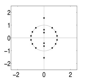
(a) $\mu=1$, $N=4$

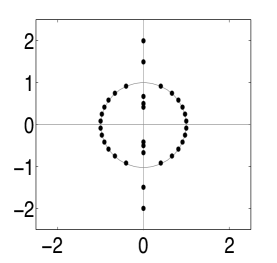
(b) $\mu=1$, $N=8$

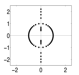
(c) $\mu=1$, $N=16$

Figure 3. Eigenvalues for reflectionless cases $\varepsilon=\varepsilon_{N}(\mu)$ (see (9)) with fixed $\mu=1$ and varying $N$. The gray circle is $|z|=1$.

The plots in figure 3 illustrate the location of eigenvalues for $\mu=1$ as $\varepsilon>0$ is varied. If $\mu$ is varied as a parameter, pairs of eigenvalues on the unit circle in the upper half-plane corresponding to a single breather may collide at $z=i$ and bifurcate off onto the imaginary axis, forming a kink-antikink pair

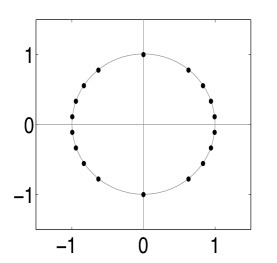
(a) $\mu=0$, $N=4$

(b) $\mu=0.8$, $N=4$

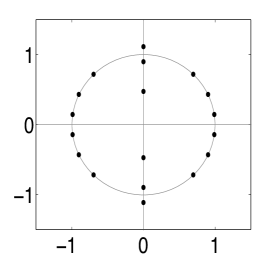
(c) $\mu=0.82$, $N=4$

Figure 4. Bifurcation of a breather quartet into a kink-antikink pair in reflectionless cases with $\varepsilon=\varepsilon_{N}(\mu)$ (see (9)) holding $N$ fixed and varying $\mu$. The gray circle is $|z|=1$.

(see figure 4). Note that this bifurcation preserves the total topological charge of $u$. Note also that for $\varepsilon$ and $\mu$ such that $(\gamma-1)/2\varepsilon\in\{1,2,3,\dots\}$, there exist double eigenvalues at $z=\pm i$. The existence of eigenvalues with algebraic multiplicity greater than one is worth noting. For instance, the self-adjoint Schrödinger eigenvalue problem associated with the Korteweg-de Vries equation admits only simple eigenvalues.

3. Inverse-scattering for reflectionless initial data

We now reconstruct the matrix $\mathbf{G}(z)=\mathbf{G}(z;x,t,\varepsilon,\mu)$ (see equation (199)) corresponding to the specific initial conditions (2) from the exact scattering data given in Theorem 2.10 in the reflectionless case when $\rho(z):=S_{21}(z)/S_{22}(z)\equiv 0$. We therefore fix $N\in\mathbb{Z}^{+}$ and set $\varepsilon=\varepsilon_{N}(\mu)$ (see (9)). We also assume the condition that $(\gamma-1)/2\varepsilon\notin\{1,2,3,\dots\}$ so all the eigenvalues (poles of $\mathbf{G}(z)$) are simple. Define

(105) $$M:=\left\lfloor\frac{1}{2\varepsilon}(\sqrt{\mu^{2}+1}-1)\right\rfloor$$

as the number of kink-antikink eigenvalue pairs. Label the eigenvalues in the closed first quadrant as follows:

1. $z_{0}=(\sqrt{\mu^{2}+1}-\mu)i$

2. $z_{n}=ie^{b}$ and $\widetilde{z}_{n}=ie^{-b}$ for $b=\text{arccosh}(\sqrt{\mu^{2}+1}-2n\varepsilon)$, $1\leq n\leq M$, $n\in\mathbb{Z}^{+}$

3. $z_{n}=e^{i\theta}$ for $\theta=\arcsin(\sqrt{\mu^{2}+1}-2n\varepsilon)$, $M+1\leq n\leq N$, $n\in\mathbb{Z}^{+}$.

Note that for the purely imaginary eigenvalues in case 2, the meaning of our notation is that $|z_{n}|>1$ while $|\widetilde{z}_{n}|<1$. In this case, $-z_{n}$ and $-\widetilde{z}_{n}$ are also eigenvalues. In case 3 on the unit circle, if $z_{n}$ is an eigenvalue then $-z_{n}^{*}$, $-z_{n}$, and $z_{n}^{*}$ are also eigenvalues.

3.1. Numerical linear algebra algorithm for reflectionless potentials

We use the conditions of the Riemann-Hilbert problem of inverse scattering (see Appendix A) to determine the matrix $\mathbf{G}(z)$ for $(x,t)\in\mathbb{R}^{2}$. In any reflectionless inverse-scattering problem, $\mathbf{G}(z)$ has no jump discontinuity across the real $z$-axis, and is therefore a meromorphic function with poles at the eigenvalues. With the assumption that the poles are simple, we may therefore expand $\mathbf{G}(z)$ in partial fractions as

(106) $$\begin{split}\mathbf{G}(z)&=\mathbb{I}+\frac{1}{z-z_{0}}\mathbf{K}_{0}^{U}+\frac{1}{z+z_{0}}\mathbf{K}_{0}^{L}\\ &\quad\quad{}+\sum_{n=1}^{M}\left\{\frac{1}{z-z_{n}}\mathbf{K}_{n}^{U}+\frac{1}{z-\widetilde{z}_{n}}\widetilde{\mathbf{K}}_{n}^{U}+\frac{1}{z+z_{n}}\mathbf{K}_{n}^{L}+\frac{1}{z+\widetilde{z}_{n}}\widetilde{\mathbf{K}}_{n}^{L}\right\}\\ &\quad\quad{}+\sum_{n=M+1}^{N}\left\{\frac{1}{z-z_{n}}\mathbf{B}_{n}^{I}+\frac{1}{z+z_{n}^{*}}\mathbf{B}_{n}^{I\!I}+\frac{1}{z+z_{n}}\mathbf{B}_{n}^{I\!I\!I}+\frac{1}{z-z_{n}^{*}}\mathbf{B}_{n}^{IV}\right\}.\end{split}$$

The superscripts on the constant matrices $\mathbf{K}_{n}^{U}$, $\widetilde{\mathbf{K}}_{n}^{U}$, $\mathbf{K}_{n}^{L}$, and $\widetilde{\mathbf{K}}_{n}^{L}$ associated with the kink or antikink eigenvalues indicate if the associated eigenvalue is in the upper or lower half-plane, and the superscripts on the constant matrices $\mathbf{B}_{n}^{I}$, $\mathbf{B}_{n}^{I\!I}$, $\mathbf{B}_{n}^{I\!I\!I}$, and $\mathbf{B}_{n}^{IV}$ associated with the breather eigenvalues indicate the quadrant of the associated eigenvalue. The residue conditions (201) show immediately that the second columns of $\mathbf{K}_{n}^{U}$, $\widetilde{\mathbf{K}}_{n}^{U}$, $\mathbf{B}_{n}^{I}$, and $\mathbf{B}_{n}^{I\!I}$ and the first columns of $\mathbf{K}_{n}^{L}$, $\widetilde{\mathbf{K}}_{n}^{L}$, $\mathbf{B}_{n}^{I\!I\!I}$, and $\mathbf{B}_{n}^{IV}$ vanish for all $n$. Write

(107) $$\mathbf{K}_{n}^{U}=\begin{bmatrix}p_{n}^{U}&0\\ q_{n}^{U}&0\end{bmatrix},\quad\widetilde{\mathbf{K}}_{n}^{U}=\begin{bmatrix}\widetilde{p}_{n}^{U}&0\\ \widetilde{q}_{n}^{U}&0\end{bmatrix},\quad\mathbf{K}_{n}^{L}=\begin{bmatrix}0&p_{n}^{L}\\ 0&q_{n}^{L}\end{bmatrix},\quad\widetilde{\mathbf{K}}_{n}^{L}=\begin{bmatrix}0&\widetilde{p}_{n}^{L}\\ 0&\widetilde{q}_{n}^{L}\end{bmatrix}$$

for $1\leq n\leq M$ and $n=0$ when applicable, and

(108) $$\mathbf{B}_{n}^{I}=\begin{bmatrix}p_{n}^{I}&0\\ q_{n}^{I}&0\end{bmatrix},\quad\mathbf{B}_{n}^{I\!I}=\begin{bmatrix}p_{n}^{I\!I}&0\\ q_{n}^{I\!I}&0\end{bmatrix},\quad\mathbf{B}_{n}^{I\!I\!I}=\begin{bmatrix}0&p_{n}^{I\!I\!I}\\ 0&q_{n}^{I\!I\!I}\end{bmatrix},\quad\mathbf{B}_{n}^{IV}=\begin{bmatrix}0&p_{n}^{IV}\\ 0&q_{n}^{IV}\end{bmatrix}.$$

for $M+1\leq n\leq N$. From the symmetries of equation (181) it follows that

$$\mathbf{K}_{n}^{U}=-\sigma_{2}\mathbf{K}_{n}^{L}\sigma_{2},\quad 0\leq n\leq M\hskip 72.26999pt$$

(109) $$\widetilde{\mathbf{K}}_{n}^{U}=-\sigma_{2}\widetilde{\mathbf{K}}_{n}^{L}\sigma_{2},\quad 1\leq n\leq M\hskip 72.26999pt$$

$$\mathbf{B}_{n}^{I}=-\mathbf{B}_{n}^{I\!I*}=-\sigma_{2}\mathbf{B}_{n}^{I\!I\!I}\sigma_{2}=\sigma_{2}\mathbf{B}_{n}^{IV*}\sigma_{2},\quad M+1\leq n\leq N.$$

Note that the elements of $\mathbf{K}_{n}^{U}$, $\widetilde{\mathbf{K}}_{n}^{U}$, $\mathbf{K}_{n}^{L}$, and $\widetilde{\mathbf{K}}_{n}^{L}$ are all imaginary. These symmetries show that the elements of the second row of $\mathbf{G}(z)$ can be expressed in terms of the elements of the first row, so to build $\mathbf{G}(z)$ it is sufficient to find the first row. Moreover, according to Proposition A.16, the potential $u$ may be recovered from the first row of $\mathbf{G}(z)$, and in terms of the partial-fraction expansion (106) this results in the formulae

(110) $$\cos(u)=1-2\left(\sum_{n=0}^{M}\frac{p_{n}^{L}}{z_{n}}+\sum_{n=M+1}^{N}\frac{p_{n}^{I\!I\!I}}{z_{n}}+\sum_{n=1}^{M}\frac{\widetilde{p}_{n}^{L}}{\widetilde{z}_{n}}+\sum_{n=M+1}^{N}\frac{p_{n}^{IV}}{-z_{n}^{*}}\right)^{2}$$

(111) $$\begin{split}\sin(u)=-2\left(1+\sum_{n=0}^{M}\frac{p_{n}^{U}}{-z_{n}}+\sum_{n=M+1}^{N}\frac{p_{n}^{I}}{-z_{n}}+\sum_{n=1}^{M}\frac{\widetilde{p}_{n}^{U}}{-\widetilde{z}_{n}}+\sum_{n=M+1}^{N}\frac{p_{n}^{I\!I}}{z_{n}^{*}}\right)\hskip 21.68121pt\\ \cdot\left(\sum_{n=0}^{M}\frac{p_{n}^{L}}{z_{n}}+\sum_{n=M+1}^{N}\frac{p_{n}^{I\!I\!I}}{z_{n}}+\sum_{n=1}^{M}\frac{\widetilde{p}_{n}^{L}}{\widetilde{z}_{n}}+\sum_{n=M+1}^{N}\frac{p_{n}^{IV}}{-z_{n}^{*}}\right).\end{split}$$

Recall that each eigenvalue $z_{n}$ in the upper half-plane has an associated modified proportionality constant $c_{n}$ which depends parametrically on $x$ and $t$ via an exponential factor. We denote by $\{\widetilde{c}_{n}\}$ those modified proportionality constants associated with the eigenvalues labeled $\{\widetilde{z}_{n}\}$. Define the vectors

(112) $$\begin{split}\mathbf{a}&:=[c_{0},c_{1},\dots,c_{N},\widetilde{c}_{1},\dots,\widetilde{c}_{M},-c_{M+1}^{*},\dots,-c_{N}^{*}]^{\mathsf{T}}\,,\\ \mathbf{w}&:=[z_{0},z_{1},\dots,z_{N},\widetilde{z}_{1},\dots,\widetilde{z}_{M},-z_{M+1}^{*},\dots,-z_{N}^{*}]^{\mathsf{T}}\,,\\ \mathbf{p}^{(1)}&:=[p_{0}^{U},\dots,p_{M}^{U},p_{M+1}^{I},\dots,p_{N}^{I},\widetilde{p}_{1}^{U},\dots,\widetilde{p}_{M}^{U},p_{M+1}^{I\!I},\dots,p_{N}^{I\!I}]^{\mathsf{T}}\,,\\ \mathbf{p}^{(2)}&:=[p_{0}^{L},\dots,p_{M}^{L},p_{M+1}^{I\!I\!I},\dots,p_{N}^{I\!I\!I},\widetilde{p}_{1}^{L},\dots,\widetilde{p}_{M}^{L},p_{M+1}^{IV},\dots,p_{N}^{IV}]^{\mathsf{T}}\,.\end{split}$$

Applying the residue conditions (201) to the partial fraction expansion (106) yields a linear inhomogeneous system for $\mathbf{p}^{(1)}$ and $\mathbf{p}^{(2)}$:

(113) $$\begin{bmatrix}\mathbb{I}_{2N+1}&\mathbf{F}\\ -\mathbf{F}&\mathbb{I}_{2N+1}\end{bmatrix}\begin{bmatrix}\mathbf{p}^{(1)}\\ \mathbf{p}^{(2)}\end{bmatrix}=\begin{bmatrix}\mathbf{0}_{2N+1}\\ \mathbf{a}\end{bmatrix}\,,\quad\text{where}\quad F_{ij}:=-\frac{a_{i}}{w_{i}+w_{j}}\,.$$

Here $\mathbf{0}_{2N+1}$ is the vector of zeros of length $2N+1$ and $\mathbb{I}_{2N+1}$ is the $2N+1$ by $2N+1$ identity matrix. The $(x,t)$-dependence of the coefficient matrix and the right-hand side of this linear system enters only through the modified proportionality constants making up the vector $\mathbf{a}$. Eliminating $\mathbf{p}^{(1)}$ using the first (block) row gives $\mathbf{p}^{(1)}=-\mathbf{F}\mathbf{p}^{(2)}$, and the resulting system for $\mathbf{p}^{(2)}$ is

(114) $$(\mathbb{I}+\mathbf{F}^{2})\mathbf{p}^{(2)}=\mathbf{a}.$$

With the explicit use of the discrete scattering data, all of the entries of $\mathbf{a}$ and $\mathbf{F}$ are known functions of $x$ and $t$. Thus, for any choice of $x=x_{0}$ and $t=t_{0}$, the system (113) can be solved numerically, giving (via equations (110) and (111)) the value of $u(x_{0},t_{0})$ independently of the value of $u(x,t)$ at any other $x$ or $t$ values.

3.2. Numerical results

Here we apply this procedure to study the solution of the Cauchy problem for the sine-Gordon equation (1) subject to the initial data (2) for various values of the parameters $\mu$ and $\varepsilon$ that make the scattering data reflectionless (so that $\varepsilon=\varepsilon_{N}(\mu)$ for some integer $N$). We are especially interested in the limit of large $N$, as this corresponds to the semiclassical limit of $\varepsilon\downarrow 0$.

For large $N$, the system (114) is poorly conditioned, and it is therefore necessary to compute $\mathbb{I}+\mathbf{F}^{2}$ and $\mathbf{a}$ with high precision at a given pair $(x,t)\in\mathbb{R}^{2}$ to find $\mathbf{p}^{(2)}$ and hence $u(x,t)$ to even a few decimal places of accuracy. For instance, for $N=16$, $\mu=1$, $x=0$, and $t=5$, the condition number of $\mathbb{I}+\mathbf{F}^{2}$ is approximately $3.5\times 10^{125}$, and it is necessary to use approximately 125-135 digit precision to accurately compute $u$.

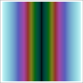
(a) $\mu=0$, $N=0$ ($\varepsilon=1$)

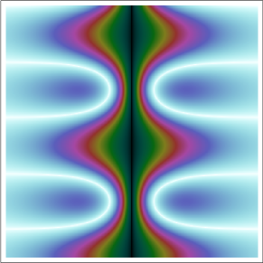
(b) $\mu=0$, $N=1$ $\left(\varepsilon=1/3\right)$

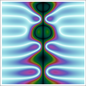
(c) $\mu=0$, $N=2$ $\left(\varepsilon=1/5\right)$

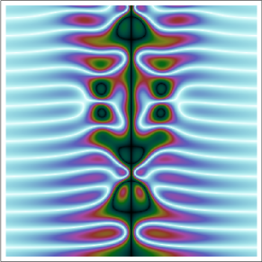
(d) $\mu=0$, $N=4$ $\left(\varepsilon=1/9\right)$

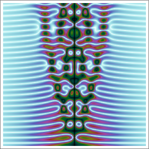
(e) $\mu=0$, $N=8$ $\left(\varepsilon=1/17\right)$

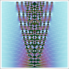
(f) $\mu=0$, $N=16$ $\left(\varepsilon=1/33\right)$

Figure 5. Plots of $\cos(u)$ for fixed $\mu=0$ and varying $N$ with $-2.5<x<2.5$ (horizontal axis) and $0<t<5$ (vertical axis).

We first study the special case of $\mu=0$. Figure 5 shows plots of the square region $-2.5<x<2.5$ and $0<t<5$ with different colors indicating different values of $\cos(u)$, with different plots corresponding to different values of $N$ varying between $N=0$ and $N=16$ ($\varepsilon=\varepsilon_{N}(0)$ between $1$ and $1/33$). Lighter colors correspond to values of $\cos(u)$ closer to $1$ and darker colors correspond to values of $\cos(u)$ closer to $-1$. The solutions of the sine-Gordon equation (1) illustrated in these plots consist of a “nonlinear superposition” of $N$ breathers and one antikink. As each associated eigenvalue lies exactly on the unit circle in the $z$-plane, the velocity of each of these soliton components, when considered in absence of the others, is exactly zero. In this sense, the solution may be considered as a zero-velocity bound state of $N$ breathers and one antikink. The most interesting phenomena are associated with the semiclassical limit $\varepsilon\downarrow 0$ equivalent to letting $N$ (the number of breathers) tend to infinity. In this limit, the plots suggest the asymptotic emergence of a fixed caustic curve $t=t(x)$ in the space-time plane separating regions containing different kinds of oscillatory behavior. Indeed, for $|x|$ sufficiently large (that is, outside of the caustic), one observes roll patterns characteristic of single-phase traveling waves. The latter are simply the exact solutions of the sine-Gordon equation obtained by substituting into (1) the traveling-wave ansatz $u(x,t)=f((kx-\omega t)/\varepsilon)$, resulting in the ordinary differential equation

(115) $$(\omega^{2}-k^{2})\frac{d^{2}f}{d\xi^{2}}+\sin(f)=0\,,\quad\quad\xi:=\varepsilon^{-1}(kx-\omega t)\,.$$

Here $k$ is the wavenumber and $\omega$ is the frequency of the traveling wave, and the waves appearing as the roll patterns in figure 5 correspond to phase velocities $c:=\omega/k$ with $|c|>1$ (which makes (115) a time-scaled version of the simple pendulum equation). The periodic solutions of (115) are expressed in terms of elliptic functions, and therefore we say that the roll patterns in figure 5 correspond to modulated waves of genus $G=1$. In the context of the phase portrait of the simple pendulum, the roll-pattern oscillations outside of the central region enclosed by the caustic curve correspond to librational motions of the pendula, i.e. orbits inside the separatrix. The sine-Gordon equation (1) also has families of exact solutions associated with hyperelliptic Riemann surfaces of arbitrarily large genus $G$, and these solutions are represented in the form $u(x,t)=f(\theta_{1}/\varepsilon,\dots,\theta_{G}/\varepsilon)$ where $\theta_{n}=k_{n}x-\omega_{n}t$ and where $f$ is a multiperiodic function of period $2\pi$ in each of its $G$ arguments. In the case $G>1$, $u$ is no longer a traveling wave, but rather is a multiphase wave. Reasoning by analogy with understood semiclassical limits of other integrable equations, we may expect that the more complicated oscillations evident in the plots of figure 5 for $t>t(x)$ (that is, inside of the caustic curve) are modulated multiphase waves for some $G>1$. Finally, we note that the caustic curve $t=t(x)$ appears to originate from the point $x=t=0$. As the velocity $u_{t}$ is zero at $t=0$ and the pendulum angle is $u=-\pi$ at $x=t=0$, the point $x=0$ is the unique point in the initial data corresponding to a point on the separatrix of the phase portrait of the simple pendulum.

(a) $\mu=1$, $N=0$ $(\varepsilon=\sqrt{2})$

(b) $\mu=1$, $N=1$ $\left(\varepsilon=\sqrt{2}/3\right)$

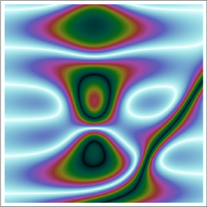
(c) $\mu=1$, $N=2$ $\left(\varepsilon=\sqrt{2}/5\right)$

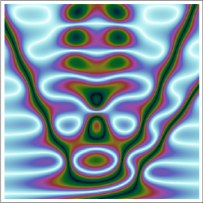
(d) $\mu=1$, $N=4$ $\left(\varepsilon=\sqrt{2}/9\right)$

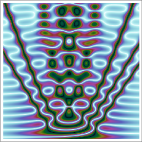
(e) $\mu=1$, $N=8$ $\left(\varepsilon=\sqrt{2}/17\right)$

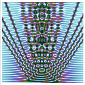
(f) $\mu=1$, $N=16$ $\left(\varepsilon=\sqrt{2}/33\right)$

Figure 6. Plots of $\cos(u)$ for fixed $\mu=1$ and varying $N$ for $-2.5<x<2.5$ (horizontal axis) and $0<t<5$ (vertical axis).

The evolution of the initial data (2) for $\mu\neq 0$ is depicted in the plots shown in figure 6. These plots are analogous to those in figure 5, except that we set $\mu=1$ and considered $\varepsilon=\varepsilon_{N}(1)$. The main effect of nonzero $\mu$ on the discrete spectrum is to include, along with the quartets of eigenvalues that correspond to breathers, an asymptotically (in the limit $N\rightarrow\infty$) nonzero fraction of eigenvalues on the imaginary axis that correspond to kinks and antikinks. The velocities of the kinks and antikinks asymptotically fill out the entire range of values $(-|\mu|/\sqrt{\mu^{2}+1},|\mu|/\sqrt{\mu^{2}+1})$. There is always one more antikink than there are kinks, and the “excess” antikink (corresponding to the eigenvalue $z_{0}=(\sqrt{2}-1)i$) carries the topological charge. This excess antikink always moves to the right (this is a consequence of $\mu>0$, it turns out), and the kink-antikink pairs corresponding to the other eigenvalues on the imaginary axis are shed periodically in time and move to the left and right. As $\varepsilon\downarrow 0$, the outermost kinks or antikinks form a caustic curve separating the modulated single-phase waves outside from a region of the space-time containing the kink/antikink trains. As these trains propagate outwards over a field of modulated single-phase waves, it seems reasonable to suppose that the pattern in this part of the space-time would be described by a modulated multiphase wave of genus $G=2$ that may be viewed as a nonlinear superposition of the single-phase waves ($G=1$) and a kink or antikink train (also $G=1$, although via orbits of (115) in the case $\omega^{2}/k^{2}<1$ that lie outside of the separatrix). That the antikinks are moving to the right while the kinks are moving to the left (for these plots corresponding to $\mu=1>0$) can be seen from a plot of $u$ itself reconstructed from its sine and cosine subject to the boundary condition $u(-\infty,t)=0$ as shown in figure 7.

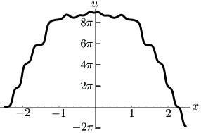
Figure 7. Plot of $u$ for $t=2.5$, $-2.5<x<2.5$, $N=16$, $\mu=1$ $\left(\varepsilon=\sqrt{2}/33\right)$.

This plot corresponds to a horizontal slice of figure 6(f) (or 8(c) below), and it is completely clear that the kinks occupy the left-hand portion of the plot (in which from figure 6(f) we see that the waves are propagating to the left) while the antikinks occupy the right-hand portion (and by similar observations are propagating to the right).

The caustic curve simultaneously emerges at $t=0$ from two (asymptotically) symmetric nonzero points $x$, and again these points admit an interpretation in terms of the separatrix of the simple pendulum equation (see below). Between these $G=2$ regions there is a triangular region containing pure single-phase oscillations that persists for a time independent of $N$. In the context of the phase portrait of the simple pendulum, these oscillations correspond to rotational motions of the pendula, i.e. orbits outside the separatrix. The collision of the two $G=2$ regions at the top of the triangular $G=1$ (rotational) region results in a region containing more complicated oscillations that resembles the region inside the caustic curve for $\mu=0$ as seen in figure 5. Note, however, that the oscillations occupying this central region may be expected to be even more complicated than those present for $\mu=0$ because there are many kinks/antikinks with very small velocities, and these will (if $N$ is sufficiently large) begin to interfere with the bound state of breathers. Finally, note that, while for $\mu\neq 0$ the exact solutions are not symmetric about $x=0$, the asymptotic behavior evidently becomes symmetric as $\varepsilon\downarrow 0$.

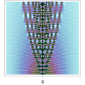
(a) $\mu=0$, $N=16$

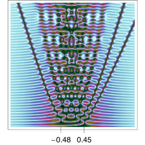
(b) $\mu=1/2$, $N=16$

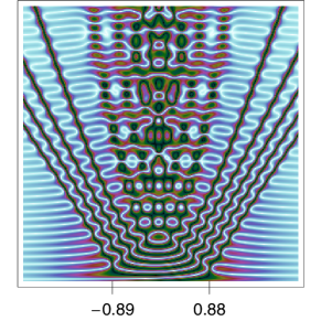
(c) $\mu=1$, $N=16$

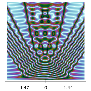
(d) $\mu=2$, $N=16$

Figure 8. Plots of $\cos(u)$ for various $\mu$ with $-1.5<x<1.5$ (horizontal axis), $0<t<5$ (vertical axis), and $N=16$.

The effect of varying $\mu$ can be seen from the plots shown in figure 8. Here, $N$ is fixed at the value $N=16$ and $\mu$ is varied, with $\varepsilon=\varepsilon_{16}(\mu)$ holding to ensure a reflectionless potential. Note that the base of the triangular region of the space-time containing single-phase rotational oscillations appears to increase with $\mu$. The ratio $M/(N-M)$ of eigenvalue quartets corresponding to kink-antikink pairs to eigenvalue quartets corresponding to breathers (see (105)) also increases as $\mu$ increases for fixed $N$, an effect that is clearly visible in the plots of figure 8.

The plots in figure 8 also contain annotation indicating our best guesses as to the values of $x$ from which the primary caustic curve emerges at $t=0$. These $x$-values may be predicted by the following simple argument. Let us rewrite the sine-Gordon equation (1) as a perturbed simple pendulum equation in first-order form:

(116) $$\varepsilon\frac{du}{dt}=v\,,\quad\quad\varepsilon\frac{dv}{dt}=-\sin(u)+\varepsilon^{2}F(t;x)$$

with forcing term $F(t;x):=u_{xx}(x,t)$. We think of $u$ and $v$ as the angle and angular velocity of a pendulum indexed by a parameter $x$. At the initial instant of time $t=0$, the function $u$ is smooth and independent of $\varepsilon$, so the perturbation term $\varepsilon^{2}F(t;x)$ is very small, and one expects $u(x,t)$ to evolve nearly independently for different values of $x\in\mathbb{R}$. This situation of independent pendulum motions might be expected to persist until $u$ develops rapidly-varying features of characteristic length proportional to $\varepsilon$, for in such a situation we would have $u_{xx}\sim\varepsilon^{-2}$ and hence the perturbation term is no longer negligible compared with $\sin(u)$. Now, at any fixed time $t$, we may plot the phase points $(u,v)$ in the phase portrait of the simple pendulum (that is, of (116) with $F\equiv 0$), and this data will appear as a curve parametrized by $x$. Figure 9 shows the initial data (2) plotted parametrically in the phase portrait of the simple pendulum for $\mu=0$, $\mu=\pm 1/2$, $\mu=\pm 1$, and $\mu=\pm 2$ (blue curves).

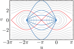
Figure 9. The initial data (2) plotted for $\mu=0$, $\mu=\pm 1/2$, $\mu=\pm 1$, and $\mu=\pm 2$ in the phase portrait of the simple pendulum.

The separatrix for the simple pendulum equation is shown with red curves. It is clear that each blue curve intersects the separatrix at exactly two points, and moreover, by unraveling the parametrization it is easy to see that these two points correspond to two distinct values of $x$. Near these values of $x$, there are pendula undergoing librational motions as well as pendula undergoing rotational motions. This is the scenario under which the most rapid amplification of the difference of angles $u$ for neighboring pendula is to be expected. Therefore, we may make the prediction that the modulated single-phase ansatz should break down immediately at $t=0$ at exactly the two values of $x$ at which the initial data meets the separatrix. These values of $x$ are easily calculated. Indeed, the separatrix is given by the equation $v=\pm 2\cos(u/2)$, and the initial data satisfies $\cos(u/2)=\tanh(x)$ and $v=2\mu\,\text{sech}(x)$. Therefore, the initial data curve (blue) intersects the separatrix (red) at values $x$ for which

(117) $$\mu=\pm\sinh(x)\,.$$

To confirm this reasoning, we took our best guesses for the $x$-values at which the phase transition occurs at $t=0$ as indicated on the plots in figure 8 and created a data set by combining these with the corresponding values of $\mu$. The ordered pairs $(x,\mu)$ making up this data set are plotted with black dots in figure 10 along with the curves (117) plotted in red.

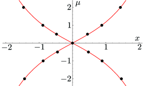
Figure 10. The relation (117) and the numerical data. The data was collected only for $\mu\geq 0$, but by a natural symmetry (see below) we may include the point $(-x,-\mu)$ whenever we measure the point $(x,\mu)$. This plot suggests that an important role is played by the separatrix of the simple pendulum in the development of caustics for the semiclassical sine-Gordon equation.

It is clear that this theory provides an accurate prediction of the points $x$ from which the caustics emerge at time $t=0$. While we have only given a comparison with the theory for initial conditions of the special form (2), it seems reasonable that the principle should be the same for more general initial data. That is, one should locate the $x$-values at which the pair $(u=f(x),v=g(x))$ lies on the separatrix $v=\pm 2\cos(u/2)$ and expect complicated oscillations to emerge from these points for $t>0$ in the semiclassical limit.

We have only computed solutions corresponding to the initial data (2) for $\mu\geq 0$. That this is sufficient follows from a simple symmetry between $\mu$ and $-\mu$. Indeed, write (1) and (2) in first-order form as

(118) $$\begin{split}\varepsilon u_{t}&=v\\ \varepsilon v_{t}&=\varepsilon^{2}u_{xx}-\sin(u)\end{split}$$

subject to the initial data

(119) $$u(x,0)=f(x)\,,\quad\quad v(x,0)=2\mu\,\text{sech}(x)\,,$$

where $\sin(f/2)=\text{sech}(x)$, $\cos(f/2)=\tanh(x)$, and consider the substitutions

(120) $$V=-v,\quad U=2\pi-u,\quad X=-x,\quad T=t.$$

Then the Cauchy problem for $U$ and $V$ consists of the first-order system

(121) $$\begin{split}\varepsilon U_{T}&=V\\ \varepsilon V_{T}&=\varepsilon^{2}U_{XX}-\sin(U)\end{split}$$

subject to the initial data

(122) $$U(X,0)=F(X)\,,\quad\quad V(X,0)=-2\mu\,\text{sech}(X)\,,$$

where $\sin(F/2)=\text{sech}(X)$, $\cos(F/2)=\tanh(X)$. Therefore, $U$ satisfies the sine-Gordon equation with initial data of the form (2) but with $\mu$ replaced with $-\mu$. In terms of $\cos(u)$, replacing $\mu$ with $-\mu$ therefore simply amounts to replacing $x$ with $-x$.

4. Concluding Remarks

The main result of this paper is the exact calculation, via the theory of hypergeometric functions, of the scattering data for the noncharacteristic Cauchy problem for the semiclassical sine-Gordon equation (1) subject to the initial data (2). That this calculation is valid for all sufficiently small $\varepsilon$ means that the formulae for the scattering data given in Theorem 2.10 may be used to formulate a corresponding inverse-scattering problem whose solution will give detailed information about the semiclassical limit of the sine-Gordon Cauchy problem. Moreover, since for each value of the parameter $\mu\in\mathbb{R}$ appearing in the initial data (2) there exists a sequence $\{\varepsilon=\varepsilon_{N}(\mu)\}_{N=1}^{\infty}$ of values of $\varepsilon$ tending to zero for which the scattering data are reflectionless, it is possible to approach the semiclassical limit in such a way that the inverse-scattering problem involves, for each $N$, only finite-dimensional linear algebra. As we have shown in Section 3, this fact makes it quite feasible to use numerical methods to solve the inverse-scattering problem for fairly large values of $N$ and therefore study the semiclassical limit, at least in a qualitative sense. Our numerical reconstructions of the exact solutions of the Cauchy problem indeed reveal marvelous structures apparently emerging in the semiclassical limit.

Needless to say, a study of the semiclassical limit based solely on numerics of the sort described in Section 3 has practical limitations. To study the semiclassical limit really requires allowing $N$ to become arbitrarily large, and the system (114) contains $2N+1$ equations and hence will ultimately become numerically intractable for sufficiently large $N$. This difficulty is compounded on the one hand by the fact that the condition numbers of the matrices involved grow rapidly with $N$, and on the other by the necessity to use a grid spacing of order $\varepsilon$ to resolve the microstructure of the solution. In other words, to study the semiclassical limit in this way, an asymptotically badly-conditioned linear algebra problem in dimension proportional to $N$ must be solved on a grid of approximately $\varepsilon^{-2}\sim N^{2}$ values of $(x,t)$ in a fixed-size region.

In our opinion, the main purpose of carrying out numerical experiments like those in Section 3 is to indicate phenomena that would be of interest to study rigorously by other (analytical) methods, and to motivate such a study. For example, figures 5 and 6 clearly indicate the existence of a limiting form of the $O(1)$ scale macrostructure independent of $\varepsilon$ in the semiclassical limit. The (apparent) existence of caustic curves separating different types of oscillations requires a careful explanation, and such an explanation would be expected to also make asymptotically accurate predictions for the locations of the caustics. In integrable problems like the sine-Gordon equation, one expects the microstructure of oscillations in between the caustic curves to be described asymptotically by modulated exact multiphase solutions of the equation associated with Riemann surfaces of genus $G$. The modulation itself is expected to be described by slowly-varying (that is, independent of $\varepsilon$) fields satisfying an appropriate system of quasilinear Whitham (modulation) equations. The sine-Gordon problem is quite different from other integrable problems for which the semiclassical limit has been investigated in that it has Whitham equations of both hyperbolic and elliptic type [6, 7]. To fully analyze these phenomena from the starting point of the scattering data we give in Theorem 2.10, it is necessary to use very precise methods of asymptotic analysis for Riemann-Hilbert problems to find an asymptotic expansion for $u(x,t;\varepsilon,\mu)$ valid as $\varepsilon\downarrow 0$. Calculations of this sort, also in the discrete spectral setting (that is, reflectionless inverse-scattering as is available for this problem when $\varepsilon=\varepsilon_{N}(\mu)$), were carried out for the semiclassical focusing NLS equation (7) for a general class of initial data in [12].

True understanding of the semiclassical asymptotics of the Cauchy problem for the sine-Gordon equation ultimately requires generalizing the one-parameter family of initial data given by (2). While the special initial data (2) is quite natural, satisfying the correct boundary conditions, and incorporating effects such as nontrivial topological charge and tunable (via the parameter $\mu$) initial velocity, one may certainly pose the Cauchy problem for more general initial data $f(\cdot)$ and $g(\cdot)$ and ask for the corresponding asymptotic behavior of $u(x,t;\varepsilon)$ as $\varepsilon\downarrow 0$. One might hope that other initial conditions that are somehow close to (2) might correspond to scattering data and dynamical behavior of $u(x,t;\varepsilon)$ whose semiclassical asymptotics are similar to those of the exactly solvable case. This would indicate a kind of stability of the semiclassical limit. Furthermore, one may be interested in the semiclassical asymptotics corresponding to initial data that differ significantly from the special data (2), for example by having a topological charge that is different. Clearly, to begin to study more general initial data, it is necessary to find quantitative approximations of the corresponding scattering data. A first step towards this goal is to seek conditions on general initial data that force the eigenvalues to lie exactly on certain contours in the complex $z$-plane. For initial data satisfying such conditions, WKB analysis can be used to find a leading-order estimate in $\varepsilon$ for the scattering data, and with more work, the error of the estimate can be analyzed. For example, for the nonselfadjoint Zakharov-Shabat eigenvalue problem relevant to the focusing NLS equation (6), Klaus and Shaw [14] showed that if the initial condition $q(x,0)$ is real and monomodal, then the discrete spectrum may only lie exactly on the imaginary axis. In the semiclassical setting, this is an exact result that holds for all $\varepsilon>0$. WKB calculations based on the Klaus-Shaw result were used in [12] to analyze certain so-called semiclassical soliton ensembles. As for sine-Gordon, Bronski and Johnson [2] recently found a result analogous to that of Klaus and Shaw, showing in particular that if $g\equiv 0$ and $f$ is monotone with topological charge $\pm 1$, then the eigenvalues must lie exactly on the unit circle in the $z$-plane. A quantitative approach to the discrete spectrum for initial data of the Bronski-Johnson type would be to map it onto a perturbation of the specific initial data (2) with $\mu=0$ (which is, of course, a special case of a Bronski-Johnson potential) using a Langer transformation, and to control the error introduced by the perturbation for small $\varepsilon$. This will be carried out in future work.

We conclude by drawing some comparisons between our results and those of Tovbis and Venakides [21] for the nonselfadjoint Zakharov-Shabat problem associated with the focusing NLS equation. The class of Tovbis-Venakides potentials (see (8)) involves a parameter $\mu\in\mathbb{R}$ ($\mu=0$ is the special case studied earlier by Satsuma and Yajima [19]). In fact, we chose to use the symbol $\mu$ for the parameter in (2) precisely because this parameter plays a similar role. One immediate observation is that only in the case $\mu=0$ is the Tovbis-Venakides initial data of Klaus-Shaw type, and similarly only in the case $\mu=0$ is the initial data (2) of Bronski-Johnson type. Thus only for $\mu=0$ is one guaranteed by general arguments that the discrete spectrum is confined to a special curve in the complex plane. Another observation is that the parameter $\mu$ has a physical interpretation of velocity in both the Tovbis-Venakides family of potentials (because in the hydrodynamic variables for Schrödinger equations introduced long ago by Madelung, the velocity of the quantum-corrected fluid motion is expressed in terms of $\phi=A(x,t)e^{iS(x,t)/\varepsilon}$ by $S_{x}(x,t)$, and for the Tovbis-Venakides potentials $S$ is proportional to $\mu$ at $t=0$) and also in the family (2) of initial data for sine-Gordon (because the initial data is a solution of the advection equation with velocity $\mu/\varepsilon$ as pointed out in the Introduction). However, as one important distinction, we note that the Tovbis-Venakides potentials have the possibility of being reflectionless for certain $\varepsilon$ only for $\mu=0$, while this possibility exists for the initial data (2) for every $\mu\in\mathbb{R}$.

Appendix A The Riemann-Hilbert Approach to Inverse Scattering for Sine-Gordon

Our aim in this appendix is to present a completely self-contained theory of inverse-scattering for the sine-Gordon equation in laboratory coordinates. In particular, we show how to represent the solution of the Cauchy problem for the sine-Gordon equation with $L^{1}$-Sobolev initial data (specifically, $1-\cos(u(x,0)),$ $\sin(u(x,0)),$ $u_{x}(x,0),$ $u_{xx}(x,0),$ $u_{t}(x,0),$ $u_{tx}(x,0)\in L^{1}$) in terms of the solution of a certain matrix-valued Riemann-Hilbert problem. To ensure that various quantities used in the inverse-scattering method are well defined with desirable properties for all $t\geq 0$, we rely on a theory of the well-posedness of the Cauchy problem that may be developed independently of any inverse scattering methodology. An outline of the relevant well-posedness theory is given in Appendix B, in which we show that the class of $L^{1}$-Sobolev potentials (in the sense defined above) is preserved for all $t\geq 0$ under the evolution of the sine-Gordon equation. Many of the results to be described below have appeared in the literature in one form or another. For instance, the characterization of the Jost solutions assuming that $1-\cos(u(x,t)),$ $\sin(u(x,t)),$ $u_{x}(x,t),$ $u_{t}(x,t)\in L^{1}$ at time $t$ appeared in Kaup [13], and aspects of the Riemann-Hilbert approach to inverse scattering were worked out for initial data $f$ and $g$ in the Schwartz space by Zhou [26] and Cheng et al. [4, 3]. The well-posedness theory we present in Appendix B appears to be a new contribution to the subject.

The starting point for our analysis is the observation [13] that the sine-Gordon equation (1) is the compatibility condition for the Lax pair

(123) $$4i\varepsilon\overline{\mathbf{w}}_{x}=\overline{\mathbf{L}}\overline{\mathbf{w}}:=\begin{bmatrix}4E+z^{-1}(1-\cos(u))&-z^{-1}\sin(u)-i\varepsilon(u_{x}+u_{t})\\ -z^{-1}\sin(u)+i\varepsilon(u_{x}+u_{t})&-4E-z^{-1}(1-\cos(u))\end{bmatrix}\overline{\mathbf{w}}$$

(124) $$4i\varepsilon\overline{\mathbf{w}}_{t}=\overline{\mathbf{B}}\overline{\mathbf{w}}:=\begin{bmatrix}4D-z^{-1}(1-\cos(u))&z^{-1}\sin(u)-i\varepsilon(u_{x}+u_{t})\\ z^{-1}\sin(u)+i\varepsilon(u_{x}+u_{t})&-4D+z^{-1}(1-\cos(u))\end{bmatrix}\overline{\mathbf{w}}$$

with $D(z)$ and $E(z)$ given in (15). In other words, there exists a basis (determined, say, by specification of two linearly independent vectors $\overline{\mathbf{w}}$ at $x=t=0$) of simultaneous solutions of (123) and (124) if and only if $u=u(x,t)$ is a solution of the sine-Gordon equation (1).

The Lax pair (124)–(123) appears to have a singularity at $z=0$. However, it is possible to use a gauge transformation to move the singularity from $z=0$ to $z=\infty$ and in this way analysis for large $z$ can be continued to appropriate sets with limit point $z=0$. This gauge transformation will play an important role in our analysis.

A.1. Jost solutions of the scattering problem

We now attempt to define the Jost solutions $\overline{\mathbf{J}}^{\pm}(x)=\overline{\mathbf{J}}^{\pm}(x;z,t,\varepsilon)$ for $z\in\mathbb{R}$ as the fundamental solution matrices of the eigenvalue equation (123) normalized as

(125) $$\begin{split}\overline{\mathbf{J}}^{+}(x)=\begin{bmatrix}e^{-iEx/\varepsilon}&0\\ 0&e^{iEx/\varepsilon}\end{bmatrix}+o(1)\quad\text{ as }x\to+\infty,\\ \overline{\mathbf{J}}^{-}(x)=\begin{bmatrix}e^{-iEx/\varepsilon}&0\\ 0&e^{iEx/\varepsilon}\end{bmatrix}+o(1)\quad\text{ as }x\to-\infty.\end{split}$$

We denote the columns of $\overline{\mathbf{J}}^{\pm}(x)$ as

(126) $$\overline{\mathbf{J}}^{\pm}(x)=:[\overline{\mathbf{j}}_{1}^{\pm}(x),\overline{\mathbf{j}}_{2}^{\pm}(x)].$$

The issue at hand is to determine whether these conditions uniquely determine $\overline{\mathbf{J}}^{\pm}(x)$ when $z$ is a real number, and then to further determine what can be said for complex $z$.

To begin, we rewrite (123) in the form

(127) $$4i\varepsilon\overline{\mathbf{J}}^{\pm}_{x}=(4E\sigma_{3}+\overline{\mathbf{Q}})\overline{\mathbf{J}}^{\pm}$$

with

(128) $$\overline{\mathbf{Q}}(x;z,\varepsilon):=\begin{bmatrix}z^{-1}(1-\cos(f))&-z^{-1}\sin(f)-i(\varepsilon f^{\prime}+g)\\ -z^{-1}\sin(f)+i(\varepsilon f^{\prime}+g)&-z^{-1}(1-\cos(f))\end{bmatrix}.$$

Here $f$ is the value of $u$, and $g$ is that of $\varepsilon u_{t}$ at some fixed time $t$. The purpose of this decomposition is to separate the part of the coefficient matrix that decays (in a certain sense) as $x\to\pm\infty$ ($\overline{\mathbf{Q}}$) from a constant term ($4E\sigma_{3}$). Defining matrices

(129) $$\overline{\mathbf{M}}^{\pm}=\left[\overline{\mathbf{m}}_{1}^{\pm},\overline{\mathbf{m}}_{2}^{\pm}\right]:=\overline{\mathbf{J}}^{\pm}e^{iEx\sigma_{3}/\varepsilon},$$

or equivalently in terms of the columns,

(130) $$\overline{\mathbf{m}}_{1}^{+}=\overline{\mathbf{j}}_{1}^{+}e^{iEx/\varepsilon},\quad\overline{\mathbf{m}}_{2}^{+}=\overline{\mathbf{j}}_{2}^{+}e^{-iEx/\varepsilon},\quad\overline{\mathbf{m}}_{1}^{-}=\overline{\mathbf{j}}_{1}^{-}e^{iEx/\varepsilon},\quad\overline{\mathbf{m}}_{2}^{-}=\overline{\mathbf{j}}_{2}^{-}e^{-iEx/\varepsilon},$$

one may easily translate the differential equation (127) and boundary conditions (125) for $z\in\mathbb{R}$ into integral equations for the matrices $\overline{\mathbf{M}}^{\pm}(x;z,\varepsilon)$:

(131) $$\overline{\mathbf{M}}^{+}(x) = \begin{bmatrix}1&0\\ 0&1\end{bmatrix}-\frac{1}{4i\varepsilon}\int_{x}^{+\infty}e^{-iE(x-y)\sigma_{3}/\varepsilon}\overline{\mathbf{Q}}(y)\overline{\mathbf{M}}^{+}(y)e^{iE(x-y)\sigma_{3}/\varepsilon}dy,$$

(132) $$\overline{\mathbf{M}}^{-}(x) = \begin{bmatrix}1&0\\ 0&1\end{bmatrix}+\frac{1}{4i\varepsilon}\int_{-\infty}^{x}e^{-iE(x-y)\sigma_{3}/\varepsilon}\overline{\mathbf{Q}}(y)\overline{\mathbf{M}}^{-}(y)e^{iE(x-y)\sigma_{3}/\varepsilon}dy.$$

While these integral equations are formulated to correspond to (123) and (125) for $z\in\mathbb{R}$, we may also consider them for complex $z$. Proposition A.1 shows that the columns $\overline{\mathbf{m}}_{1}^{+}(x)$ and $\overline{\mathbf{m}}_{2}^{-}(x)$ are well-defined by (131) and (132) respectively as long as $\Im(z)\leq 0$, and moreover for each $x\in\mathbb{R}$ they are analytic for $\Im(z)<0$, and continuous in the closed lower half $z$-plane for $z$ bounded away from $z=0$. Then Proposition A.2 uses an alternate gauge to extend continuity to small $z$.

Proposition A.1.

Suppose $1-\cos(f)$, $\sin(f)$, $\varepsilon f^{\prime}+g\in L^{1}$. If $\Im(z)\leq 0$, then the first column of (131) and the second column of (132) uniquely define solutions $\overline{\mathbf{m}}_{1}^{+}(x;z)$ and $\overline{\mathbf{m}}_{2}^{-}(x;z)$. These functions are, for each $x\in\mathbb{R}$, analytic for $\Im(z)<0$ and continuous for $z\in\{|z|\geq\delta\}\cap\{\Im(z)\leq 0\}$ for each $\delta>0$.

Proof.

The function $\overline{\mathbf{m}}_{1}^{+}(x;z)$ is constructed from equation (131) via an iterative argument. Define the $0^{\text{th}}$ iterate for $\overline{\mathbf{m}}_{1}^{+}$ as $\overline{\mathbf{m}}_{1,0}^{+}(x):=[1,0]^{\mathsf{T}}$. Then define the $n^{\text{th}}$ iterate inductively by

(133) $$\overline{\mathbf{m}}_{1,n}^{+}(x):=\begin{bmatrix}1\\ 0\end{bmatrix}-\int_{x}^{+\infty}\overline{\mathbf{K}}^{+}_{1}(y;x,z)\overline{\mathbf{m}}_{1,n-1}^{+}(y)dy$$

with

(134) $$\overline{\mathbf{K}}^{+}_{1}(y)=\overline{\mathbf{K}}^{+}_{1}(y;x,z):=\frac{1}{4i\varepsilon}\begin{bmatrix}z^{-1}(1-\cos(f))&-z^{-1}\sin(f)-i(\varepsilon f^{\prime}+g)\\ \left(-z^{-1}\sin(f)+i(\varepsilon f^{\prime}+g)\right)e^{2i(x-y)E/\varepsilon}&-z^{-1}(1-\cos(f))e^{2i(x-y)E/\varepsilon}\end{bmatrix}.$$

Here $f$, $f^{\prime}$, and $g$ are functions of $y$. It follows that

(135) $$\begin{split}\overline{\mathbf{m}}_{1,n}^{+}(x)=&\begin{bmatrix}1\\ 0\end{bmatrix}-\int_{x}^{+\infty}\overline{\mathbf{K}}^{+}_{1}(x_{1})\begin{bmatrix}1\\ 0\end{bmatrix}dx_{1}+\cdots\\ &+(-1)^{n}\int_{x}^{+\infty}\int_{x_{1}}^{+\infty}\cdots\int_{x_{n-1}}^{+\infty}\overline{\mathbf{K}}^{+}_{1}(x_{1})\cdots\overline{\mathbf{K}}^{+}_{1}(x_{n})\begin{bmatrix}1\\ 0\end{bmatrix}dx_{n}\cdots dx_{1}.\end{split}$$

If the sequence $\{\overline{\mathbf{m}}_{1,n}^{+}(x)\}$ converges, then $\overline{\mathbf{m}}_{1}^{+}(x)$ will be defined as its limit, which clearly has the form of an infinite series.

Consider the $n^{\text{th}}$ term in this series. Let $\left\|\mathbf{v}\right\|:=|v_{1}|+|v_{2}|$ be the $\ell^{1}$ vector norm and $\left\|\mathbf{M}\right\|=\max(|M_{11}|+|M_{21}|,|M_{12}|+|M_{22}|)$ be the induced matrix norm. The key observation is that (because $\Im(E)\leq 0$ for $\Im(z)\leq 0$) the assumption $\Im(z)\leq 0$ implies that if $y>x$ then $\|\overline{\mathbf{K}}^{+}_{1}(y)\|$ is bounded by a linear combination of $1-\cos(f)$, $|\sin(f)|$, and $|\varepsilon f^{\prime}+g|$ with constant coefficients independent of $y$ and uniformly bounded for $|z|\geq\delta>0$. Therefore whenever $\Im(z)\leq 0$ with $z\neq 0$ we may define a function in $L^{\infty}(\mathbb{R})$ by

(136) $$\nu(x):=\int_{x}^{+\infty}\|\overline{\mathbf{K}}^{+}_{1}(y)\|dy.$$

Furthermore, $\|\nu(x)\|_{L^{\infty}}$ is uniformly bounded in $z$ for $z\in\{|z|\geq\delta\}\cap\{\Im(z)\leq 0\}$ for every $\delta>0$. Then

(137) $$\begin{split}\left\|\int_{x}^{+\infty}\int_{x_{1}}^{+\infty}\cdots\int_{x_{n-1}}^{+\infty}\right.&\left.\overline{\mathbf{K}}^{+}_{1}(x_{1})\cdots\overline{\mathbf{K}}^{+}_{1}(x_{n})\begin{bmatrix}1\\ 0\end{bmatrix}\,dx_{n}\cdots dx_{1}\right\|\\ &\leq\int^{+\infty}_{x}\int^{+\infty}_{x_{1}}\cdots\int^{+\infty}_{x_{n-1}}\|\overline{\mathbf{K}}^{+}_{1}(x_{1})\|\cdots\|\overline{\mathbf{K}}^{+}_{1}(x_{n})\|\,dx_{n}\cdots dx_{1}\\ &=\int_{0}^{\nu(x)}\int_{0}^{\nu(x_{1})}\cdots\int_{0}^{\nu(x_{n-1})}d\nu(x_{n})\cdots d\nu(x_{1})\\ &=\frac{\nu(x)^{n}}{n!}\,.\end{split}$$

It follows that the partial sums $\overline{\mathbf{m}}_{1,n}^{+}(x)$ are majorized by those of an exponential series, and so the sequence of partial sums converges and the limit furnishes the unique solution of the first column of the integral equation (131). By uniformity of the convergence, analyticity for $\Im(z)<0$ and continuity for $z\in\{|z|\geq\delta\}\cap\{\Im(z)\leq 0\}$ for each $\delta>0$ extend from the partial sums to the limit $\overline{\mathbf{m}}_{1}^{+}(x;z)$. We also have the estimate

(138) $$\|\overline{\mathbf{m}}_{1}^{+}(x)\|\leq e^{\nu(x)}\leq\exp\left(\int_{-\infty}^{+\infty}\|\overline{\mathbf{K}}^{+}_{1}(y)\|dy\right)<\infty,$$

which is uniform for $\delta>0$. The argument for $\overline{\mathbf{m}}_{2}^{-}(x;z)$ is similar. ∎

The argument in Proposition A.1 fails for $z$ near $z=0$ because of the coefficient $z^{-1}$ in the matrix entries of $\overline{\mathbf{K}}^{-}_{1}(y)$. The use of an alternate gauge, which we call the zero gauge, circumvents this problem. We define a new set of functions in terms of the Jost solutions $\overline{\mathbf{J}}^{\pm}(x)$ by

(139) $$\underline{\mathbf{J}}^{\pm}(x):=\begin{bmatrix}\displaystyle\cos\left(\frac{f(x)}{2}\right)&\displaystyle\sin\left(\frac{f(x)}{2}\right)\\ \\ \displaystyle-\sin\left(\frac{f(x)}{2}\right)&\displaystyle\cos\left(\frac{f(x)}{2}\right)\end{bmatrix}\overline{\mathbf{J}}^{\pm}(x)\,,$$

with columns $\underline{\mathbf{J}}^{\pm}(x)=:[\underline{\mathbf{j}}^{\pm}_{1}(x),\underline{\mathbf{j}}^{\pm}_{2}(x)]$. Note that this gauge transformation can be interpreted as a rotation of the Jost solution column vectors by an angle $-f(x)/2$. It follows by direct calculation that the gauge-transformed matrices $\underline{\mathbf{J}}^{\pm}(x)$ satisfy the modified eigenvalue equation

(140) $$4i\varepsilon\underline{\mathbf{J}}^{\pm}_{x}=\left(4E\sigma_{3}+\underline{\mathbf{Q}}\right)\underline{\mathbf{J}}^{\pm}$$

where

(141) $$\underline{\mathbf{Q}}:=\begin{bmatrix}-z(1-\cos(f))&-z\sin(f)+i(\varepsilon f^{\prime}-g)\\ -z\sin(f)-i(\varepsilon f^{\prime}-g)&z(1-\cos(f))\end{bmatrix}.$$

Assuming the boundary conditions

(142) $$\lim_{x\to-\infty}u(x,0)=0\quad\quad\text{and}\quad\quad\lim_{x\to+\infty}u(x,0)=2\pi n$$

hold in a suitable sense, the required behavior of $\underline{\mathbf{J}}^{\pm}(x)$ as $x\to\pm\infty$ is derived from (139) and (125):

(143) $$\begin{split}&\underline{\mathbf{J}}^{+}(x)=\begin{bmatrix}(-1)^{n+1}e^{-iEx/\varepsilon}&0\\ 0&(-1)^{n+1}e^{iEx/\varepsilon}\end{bmatrix}+o(1)\quad\text{as }x\to+\infty\text{ for }z\in\mathbb{R},\\ &\underline{\mathbf{J}}^{-}(x)=\begin{bmatrix}e^{-iEx/\varepsilon}&0\\ 0&e^{iEx/\varepsilon}\end{bmatrix}+o(1)\quad\text{as }x\to-\infty\text{ for }z\in\mathbb{R}.\end{split}$$

Analogous to equation (129), define

(144) $$\underline{\mathbf{M}}^{\pm}(x):=\underline{\mathbf{J}}^{\pm}(x)e^{iEx\sigma_{3}/\varepsilon}$$

with columns $\underline{\mathbf{M}}^{\pm}(x)=:[\underline{\mathbf{m}}_{1}^{\pm}(x),\underline{\mathbf{m}}_{2}^{\pm}(x)]$. It follows by integrating (140) using the boundary conditions (143) that $\underline{\mathbf{M}}^{\pm}(x)$ satisfy the integral equations

(145) $$\underline{\mathbf{M}}^{+}(x)=\begin{bmatrix}(-1)^{n+1}&0\\ 0&(-1)^{n+1}\end{bmatrix}-\frac{1}{4i\varepsilon}\int_{x}^{+\infty}e^{-iE(x-y)\sigma_{3}/\varepsilon}\underline{\mathbf{Q}}(y)\underline{\mathbf{M}}^{+}(y)e^{iE(x-y)\sigma_{3}/\varepsilon}dy,$$

(146) $$\underline{\mathbf{M}}^{-}(x)=\begin{bmatrix}1&0\\ 0&1\end{bmatrix}+\frac{1}{4i\varepsilon}\int_{-\infty}^{x}e^{-iE(x-y)\sigma_{3}/\varepsilon}\underline{\mathbf{Q}}(y)\underline{\mathbf{M}}^{-}(y)e^{iE(x-y)\sigma_{3}/\varepsilon}dy.$$

Now these modified integral equations for the gauge-transformed solutions $\underline{\mathbf{M}}^{\pm}(x)$ are used to show that the columns of $\overline{\mathbf{M}}^{\pm}(x)$ are continuous in a neighborhood of $z=0$ in appropriate half-planes.

Proposition A.2.

Suppose $1-\cos(f)$, $\sin(f)$, $\varepsilon f^{\prime}-g\in L^{1}$. Then for each $x\in\mathbb{R}$ and for each $\delta>0$, $\overline{\mathbf{m}}_{1}^{+}(x;z)$ and $\overline{\mathbf{m}}_{2}^{-}(x;z)$ are continuous functions of $z$ in the region $z\in\{|z|<\delta\}\cap\{\Im(z)\leq 0\}$.

Proof.

The function $\underline{\mathbf{m}}_{1}^{+}(x)$ is constructed iteratively from equation (145), similar to the construction of $\overline{\mathbf{m}}_{1}^{+}(x)$ in Proposition A.1. Set $\underline{\mathbf{m}}_{1,0}^{+}(x):=[(-1)^{n+1},0]^{\mathsf{T}}$. Define the $n^{\text{th}}$ iterate by

(147) $$\underline{\mathbf{m}}_{1,n}^{+}(x):=\begin{bmatrix}(-1)^{n+1}\\ 0\end{bmatrix}-\int_{x}^{+\infty}\underline{\mathbf{K}}^{+}_{1}(y;x,z)\underline{\mathbf{m}}_{1,n-1}^{+}(y)\,dy\,,$$

where

(148) $$\underline{\mathbf{K}}^{+}_{1}(y;x,z):=\frac{1}{4i\varepsilon}\begin{bmatrix}-z(1-\cos(f))&-z\sin(f)+i(\varepsilon f^{\prime}-g)\\ \left(-z\sin(f)-i(\varepsilon f^{\prime}-g)\right)e^{2i(x-y)E/\varepsilon}&z(1-\cos(f))e^{2i(x-y)E/\varepsilon}\end{bmatrix}.$$

Aside from the exponential factors $e^{2i(x-y)E/\varepsilon}$, everywhere that a factor of $z^{-1}$ occurred in $\overline{\mathbf{K}}^{+}_{1}(y)$ there is in $\underline{\mathbf{K}}^{+}_{1}(y)$ a factor of $z$. This allows parallel analysis as in the proof of Proposition A.1 to go through with the condition $|z|>\delta$ replaced by the condition $|z|<\delta$. Thus, the iterates converge and $\underline{\mathbf{m}}_{1}^{+}(x;z)$ is analytic in the lower half $z$-plane and continuous in the closed lower half $z$-plane for bounded $z$. A similar argument works for $\underline{\mathbf{m}}^{-}_{2}(x;z)$ as well. Finally, the gauge transformation (139) is independent of $z$ and so does not affect the continuity, and therefore $\overline{\mathbf{m}}_{1}^{+}(x;z)$ and $\overline{\mathbf{m}}_{2}^{-}(x;z)$ as defined by Proposition A.1 are in fact continuous in the whole closed lower half-plane. ∎

Together, Propositions A.1 and A.2 show $\overline{\mathbf{m}}_{1}^{+}(x;z)$ and $\overline{\mathbf{m}}_{2}^{-}(x;z)$ are analytic in the lower half $z$-plane and continuous in the closed lower half $z$-plane. An analogous result holds for $\overline{\mathbf{m}}_{1}^{-}(x;z)$ and $\overline{\mathbf{m}}_{2}^{+}(x;z)$ in the upper half-plane.

Proposition A.3.

Suppose $1-\cos(f)$, $\sin(f)$, $f^{\prime}$, $g\in L^{1}$. If $\Im(z)\geq 0$, then the first column of (132) and the second column of (131) uniquely define solutions $\overline{\mathbf{m}}_{1}^{-}(x;z)$ and $\overline{\mathbf{m}}_{2}^{+}(x;z)$. These functions are, for each $x\in\mathbb{R}$, analytic for $\Im(z)>0$ and continuous for $\Im(z)\geq 0$.

Proof.

The proof follows that of Propositions A.1 and A.2, taking into account the sign of the real part of the exponential factors in equations (131) and (132). ∎

Propositions A.2 and A.3 can be summarized as follows.

Theorem A.4 (Kaup, [13]).

Suppose $1-\cos(f),\sin(f),f^{\prime},g\in L^{1}$. Then $\overline{\mathbf{m}}_{1}^{-}(x;z)$ and $\overline{\mathbf{m}}_{2}^{+}(x;z)$ are well-defined and for each $x\in\mathbb{R}$ are continuous for $z\in\mathbb{R}$ and extend continuously to analytic functions in the upper half $z$-plane. Similarly, $\overline{\mathbf{m}}_{1}^{+}(x;z)$ and $\overline{\mathbf{m}}_{2}^{-}(x;z)$ are well-defined and for each $x\in\mathbb{R}$ are continuous for $z\in\mathbb{R}$ and extend continuously to analytic functions in the lower half $z$-plane.

Next we establish a lemma showing that under the assumption of a little more smoothness of the potentials, the $x$ derivatives of the columns of $\overline{\mathbf{M}}^{\pm}(x)$ are, for each fixed $x\in\mathbb{R}$, uniformly bounded in the appropriate closed half-planes for $z$.

Lemma A.5.

Suppose $1-\cos(f),\sin(f),f^{\prime},f^{\prime\prime},g,g^{\prime}\in L^{1}$. Then $\overline{\mathbf{m}}_{1x}^{+}(x;z)$ and $\overline{\mathbf{m}}_{2x}^{-}(x;z)$ are uniformly bounded in $x$ for each fixed $z$ with $\Im(z)\leq 0$, having $L^{\infty}$ norms that are uniformly bounded for all such $z$. Similarly, $\overline{\mathbf{m}}_{1x}^{-}(x;z)$ and $\overline{\mathbf{m}}_{2x}^{+}(x;z)$ are uniformly bounded in $x$ for each fixed $z$ with $\Im(z)\geq 0$, having $L^{\infty}$ norms that are uniformly bounded for all such $z$.

Proof.

We show the result for $\overline{\mathbf{m}}_{1x}^{+}$. The proofs of the results for $\overline{\mathbf{m}}_{2x}^{-}$, $\overline{\mathbf{m}}_{1x}^{-}$, and $\overline{\mathbf{m}}_{2x}^{+}$ are similar. Choose $z$ such that $\Im(z)\leq 0$. From (131), $\overline{\mathbf{m}}_{1}^{+}$ satisfies the integral equation

(149) $$\overline{\mathbf{m}}_{1}^{+}(x;z)=\begin{bmatrix}1\\ 0\end{bmatrix}-\int_{x}^{+\infty}\overline{\mathbf{K}}_{1}^{+}(y;x,z)\overline{\mathbf{m}}_{1}^{+}(y;z)\,dy$$

with $\overline{\mathbf{K}}_{1}^{+}$ defined by (134). We write the entries of $\overline{\mathbf{Q}}$ and $\overline{\mathbf{m}}_{1}^{+}$ as

(150) $$\overline{\mathbf{Q}}=:\begin{bmatrix}\overline{Q}_{11}&\overline{Q}_{12}\\ \overline{Q}_{21}&\overline{Q}_{22}\end{bmatrix},\quad\overline{\mathbf{m}}_{1}^{+}=:\begin{bmatrix}\overline{m}_{11}^{+}\\ \overline{m}_{21}^{+}\end{bmatrix}.$$

The first entry of (149) is

(151) $$\overline{m}_{11}^{+}(x;z)=1-\frac{1}{4i\varepsilon}\int_{x}^{+\infty}\overline{Q}_{11}^{+}(y;z)\overline{m}_{11}^{+}(y;z)+\overline{Q}_{12}^{+}(y;z)\overline{m}_{21}^{+}(y;z)\,dy,$$

and differentiation in $x$ gives

(152) $$\overline{m}_{11x}^{+}(x;z)=\frac{1}{4i\varepsilon}[\overline{Q}_{11}^{+}(x;z)\overline{m}_{11}^{+}(x;z)+\overline{Q}_{12}^{+}(x;z)\overline{m}_{21}^{+}(x;z)].$$

Thus $\overline{m}_{11x}^{+}(x;z)$ is uniformly bounded in $x$ with $L^{\infty}$ norm uniformly bounded for $z\in\{|z|>\delta\}\cap\{\Im(z)\leq 0\}$ because $\overline{\mathbf{m}}_{1}^{+}$ and $\overline{\mathbf{Q}}$ are (we see that $f^{\prime},g\in L^{\infty}$ by noting $f^{\prime\prime},g^{\prime}\in L^{1}$ by assumption and applying the fundamental theorem of calculus). The second entry of (149) is

(153) $$\overline{m}_{21}^{+}(x;z)=-\frac{1}{4i\varepsilon}\int_{x}^{+\infty}e^{2iE(x-y)/\varepsilon}[\overline{Q}_{21}(y;z)\overline{m}_{11}^{+}(y;z)+\overline{Q}_{22}(y;z)\overline{m}_{21}^{+}(y;z)]\,dy.$$

Taking an $x$-derivative gives

(154) $$\begin{split}\overline{m}_{21x}^{+}(x;z)=&\;\frac{1}{4i\varepsilon}[\overline{Q}_{21}(x;z)\overline{m}_{11}^{+}(x;z)+\overline{Q}_{22}(x;z)\overline{m}_{21}^{+}(x;z)]\\ &\;-\frac{1}{4i\varepsilon}\int_{x}^{+\infty}\frac{2iE}{\varepsilon}e^{2iE(x-y)/\varepsilon}[\overline{Q}_{21}(y;z)\overline{m}_{11}^{+}(y;z)+\overline{Q}_{22}(y;z)\overline{m}_{21}^{+}(y;z)]\,dy\\ =&\;\frac{1}{4i\varepsilon}[\overline{Q}_{21}(x;z)\overline{m}_{11}^{+}(x;z)+\overline{Q}_{22}(x;z)\overline{m}_{21}^{+}(x;z)]\\ &\;+\frac{1}{4i\varepsilon}\int_{x}^{+\infty}\frac{d}{dy}\left(e^{2iE(x-y)/\varepsilon}\right)[\overline{Q}_{21}(y;z)\overline{m}_{11}^{+}(y;z)+\overline{Q}_{22}(y;z)\overline{m}_{21}^{+}(y;z)]\,dy.\end{split}$$

Now (for $y>x$ and in the indicated region of the $z$-plane) we have $\exp(2iE(x-y)/\varepsilon),\overline{m}_{11}^{+},\overline{m}_{21}^{+}\in L^{\infty}$. Also, $\overline{\mathbf{Q}}\to 0$ as $x\to\pm\infty$. To see this, note that the limiting value of $f_{x}$ exists as $x\rightarrow\pm\infty$ because $f_{xx}\in L^{1}$, and moreover since $f_{x}\in L^{1}$ both limits must be zero. The same reasoning holds for $1-\cos(f)$, $\sin(f)$, and $g$. Therefore,

(155) $$\lim_{x\to\pm\infty}1-\cos(f)=0,\quad\lim_{x\to\pm\infty}\sin(f)=0,\quad\lim_{x\to\pm\infty}f_{x}=0,\quad\lim_{x\to\pm\infty}g=0.$$

Thus $\exp(2iE(x-y)/\varepsilon)[\overline{Q}_{21}(y)\overline{m}_{11}^{+}(y)+\overline{Q}_{22}(y)\overline{m}_{21}^{+}(y)]\to 0$ as $y\to+\infty$, and so integrating by parts and distributing the $y$-derivative gives

(156) $$\begin{split}\overline{m}_{21x}^{+}(x;z)=&-\frac{1}{4i\varepsilon}\int_{x}^{+\infty}e^{2iE(x-y)/\varepsilon}[\overline{Q}_{21y}(y;z)\overline{m}_{11}^{+}(y;z)+\overline{Q}_{21}(y;z)\overline{m}_{11y}^{+}(y;z)+\overline{Q}_{22y}(y;z)\overline{m}_{21}^{+}(y;z)]dy\\ &-\frac{1}{4i\varepsilon}\int_{x}^{+\infty}e^{2iE(x-y)/\varepsilon}\overline{Q}_{22}(y;z)\overline{m}_{21y}^{+}(y;z)dy\\ =:&\;I(x)-\int_{x}^{+\infty}J(y;x,z)\overline{m}_{21y}^{+}(y;z)dy.\end{split}$$

Note that $I(x)$ is uniformly bounded in $x$ with $L^{\infty}$ norm uniformly bounded for $z\in\{|z|<\delta\}\cap\{\Im(z)\leq 0\}$ and that $J\in L^{1}$ with norm uniformly bounded for $z\in\{|z|<\delta\}\cap\{\Im(z)\leq 0\}$. Therefore, by an iteration argument as in the proof of Proposition A.1,

(157) $$\|m_{21x}^{+}\|_{L^{\infty}}\leq\|I\|_{L^{\infty}}\exp\left(\int_{-\infty}^{+\infty}|J(y)|\,dy\right)<\infty$$

where the bound is uniform for $z\in\{|z|<\delta\}\cap\{\Im(z)\leq 0\}$. The uniform bound for $z\in\{|z|>\delta\}\cap\{\Im(z)\leq 0\}$ is shown similarly using the zero gauge defined by (139). ∎

The assumption of additional smoothness of the potentials as above also provides limiting values of the columns of $\overline{\mathbf{M}}^{\pm}(x;z)$ in various situations.

Proposition A.6.

Suppose $1-\cos(f),\sin(f),f^{\prime},f^{\prime\prime},g,g^{\prime}\in L^{1}$. Then the columns of $\overline{\mathbf{M}}^{\pm}(x;z)$ have the following limits in $x$ and $z$:

(158) $$\mathop{\lim_{x\to+\infty}}_{\Im(z)\leq 0}\overline{\mathbf{m}}_{1}^{+}(x;z)=\begin{bmatrix}1\\ 0\end{bmatrix},\quad\mathop{\lim_{x\to-\infty}}_{\Im(z)\leq 0}\overline{\mathbf{m}}_{2}^{-}(x;z)=\begin{bmatrix}0\\ 1\end{bmatrix},\quad\mathop{\lim_{x\to-\infty}}_{\Im(z)\geq 0}\overline{\mathbf{m}}_{1}^{-}(x;z)=\begin{bmatrix}1\\ 0\end{bmatrix},\quad\mathop{\lim_{x\to+\infty}}_{\Im(z)\geq 0}\overline{\mathbf{m}}_{2}^{+}(x;z)=\begin{bmatrix}0\\ 1\end{bmatrix},$$

(159) $$\mathop{\lim_{z\to\infty}}_{\Im(z)\leq 0}\overline{\mathbf{m}}_{1}^{+}(x;z)=\begin{bmatrix}1\\ 0\end{bmatrix},\quad\mathop{\lim_{z\to\infty}}_{\Im(z)\leq 0}\overline{\mathbf{m}}_{2}^{-}(x;z)=\begin{bmatrix}0\\ 1\end{bmatrix},\quad\mathop{\lim_{z\to\infty}}_{\Im(z)\geq 0}\overline{\mathbf{m}}_{1}^{-}(x;z)=\begin{bmatrix}1\\ 0\end{bmatrix},\quad\mathop{\lim_{z\to\infty}}_{\Im(z)\geq 0}\overline{\mathbf{m}}_{2}^{+}(x;z)=\begin{bmatrix}0\\ 1\end{bmatrix},$$

(160) $$\begin{split}\mathop{\lim_{z\to 0}}_{\Im(z)\leq 0}\overline{\mathbf{m}}_{1}^{+}(x;z)=(-1)^{n+1}\begin{bmatrix}\displaystyle\cos\left(\frac{f(x)}{2}\right)\vspace{0.1 in}\\ \displaystyle\sin\left(\frac{f(x)}{2}\right)\end{bmatrix},\quad\mathop{\lim_{z\to 0}}_{\Im(z)\leq 0}\overline{\mathbf{m}}_{2}^{-}(x;z)=\begin{bmatrix}\displaystyle-\sin\left(\frac{f(x)}{2}\right)\vspace{0.1 in}\\ \displaystyle\cos\left(\frac{f(x)}{2}\right)\end{bmatrix},\\ \mathop{\lim_{z\to 0}}_{\Im(z)\geq 0}\overline{\mathbf{m}}_{1}^{-}(x;z)=\begin{bmatrix}\displaystyle\cos\left(\frac{f(x)}{2}\right)\vspace{0.1 in}\\ \displaystyle\sin\left(\frac{f(x)}{2}\right)\end{bmatrix},\quad\mathop{\lim_{z\to 0}}_{\Im(z)\geq 0}\overline{\mathbf{m}}_{2}^{+}(x;z)=(-1)^{n+1}\begin{bmatrix}\displaystyle-\sin\left(\frac{f(x)}{2}\right)\vspace{0.1 in}\\ \displaystyle\cos\left(\frac{f(x)}{2}\right)\end{bmatrix}.\end{split}$$

Proof.

We will prove the statements concerning $\overline{\mathbf{m}}_{1}^{+}(x;z)$; the proofs of the corresponding limits for $\overline{\mathbf{m}}_{1}^{-}(x;z)$, $\overline{\mathbf{m}}_{2}^{+}(x;z)$, and $\overline{\mathbf{m}}_{2}^{-}(x;z)$ are similar.

We first establish the limit in $x$. Fix $z\in\{|z|>\delta\}\cap\{\Im(z)\leq 0\}$ for some fixed $\delta>0$. Consider the integral equation (149) for $\overline{\mathbf{m}}_{1}^{+}(x;z)$. The product $\overline{\mathbf{K}}_{1}^{+}\overline{\mathbf{m}}_{1}^{+}\in L^{1}$ as a function of $y$ since $|z|>\delta$, since $\cos(f)-1,\sin(f),f^{\prime},g\in L^{1}$, and since $\overline{\mathbf{m}}_{1}^{+}\in L^{\infty}$ for $z\in\{|z|>\delta\}\cap\{\Im(z)\leq 0\}$. Furthermore, $\overline{\mathbf{K}}_{1}^{+}\overline{\mathbf{m}}_{1}^{+}\chi_{[x,+\infty)}$ tends to zero pointwise in $y$ as $x\to+\infty$. Therefore the limit for $\overline{\mathbf{m}}_{1}^{+}(x;z)$ as $x\to+\infty$ holds by dominated convergence for $z\in\{|z|>\delta\}\cap\{\Im(z)\leq 0\}$. The result for $z\in\{|z|<\delta\}\cap\{\Im(z)\leq 0\}$ holds by the same reasoning applied to the integral equation

(161) $$\underline{\mathbf{m}}_{1}^{+}(x;z):=\begin{bmatrix}(-1)^{n+1}\\ 0\end{bmatrix}-\int_{x}^{+\infty}\underline{\mathbf{K}}^{+}_{1}(y;x,z)\underline{\mathbf{m}}_{1}^{+}(y;z)\,dy,$$

written in the zero gauge with $\underline{\mathbf{K}}_{1}^{+}$ given by (148), and the use of the gauge transformation (139) to go back to $\overline{\mathbf{m}}_{1}^{+}(x;z)$.

Next consider the limit of $\overline{\mathbf{m}}_{1}^{+}(x;z)$ as $z\to\infty$ for $\Im(z)\leq 0$. The second entry of (149) may be written as

(162) $$\overline{m}_{21}^{+}(x;z)=\frac{1}{4i\varepsilon}\int_{x}^{+\infty}\frac{d}{dy}\left(\frac{\varepsilon}{2iE}e^{2iE(x-y)/\varepsilon}\right)[\overline{Q}_{21}(y;z)\overline{m}_{11}^{+}(y;z)+\overline{Q}_{22}(y;z)\overline{m}_{21}^{+}(y;z)]\,dy.$$

Integration by parts gives

(163) $$\begin{split}\overline{m}_{21}^{+}(x;z)=&\frac{1}{8E}[\overline{Q}_{21}(x;z)\overline{m}_{11}^{+}(x;z)+\overline{Q}_{22}(x;z)\overline{m}_{21}^{+}(x;z)]\\ &+\int_{x}^{+\infty}\frac{1}{8E}e^{2iE(x-y)/\varepsilon}\frac{d}{dy}[\overline{Q}_{21}(y;z)\overline{m}_{11}^{+}(y;z)+\overline{Q}_{22}(y;z)\overline{m}_{21}^{+}(y;z)]\,dy.\end{split}$$

Since $f^{\prime},g\in L^{\infty}$ (because $f^{\prime\prime},g^{\prime}\in L^{1}$), we have $\overline{Q}_{21},\overline{Q}_{22}\in L^{\infty}$ for $|z|>\delta$. Since also $\overline{m}_{11}^{+}$ and $\overline{m}_{21}^{+}$ are uniformly bounded for $\Im(z)\leq 0$ by Theorem A.4, the boundary term $[\overline{Q}_{21}\overline{m}_{11}^{+}+\overline{Q}_{22}\overline{m}_{21}^{+}]/8E$ vanishes as $z\to\infty$ for $\Im(z)\leq 0$ (and hence as $E\rightarrow\infty$). As for the integral term, $\overline{Q}_{21},\overline{Q}_{21y},\overline{Q}_{22},\overline{Q}_{22y}\in L^{1}$ for $|z|>\delta$ and $e^{2iE(x-y)/\varepsilon},\overline{m}_{11}^{+},\overline{m}_{11y}^{+},\overline{m}_{21}^{+},\overline{m}_{21y}^{+}$ are uniformly bounded for $y>x$ and $\Im(z)\leq 0$. Therefore $e^{2iE(x-y)/\varepsilon}d/dy[\overline{Q}_{21}\overline{m}_{11}^{+}+\overline{Q}_{22}\overline{m}_{21}^{+}]\in L^{1}$ for $z\in\{|z|>\delta\}\cap\{\Im(z)\leq 0\}$. Since $E\rightarrow\infty$ as $z\rightarrow\infty$, the integrand tends to zero pointwise in $y$ almost everywhere as $z\to\infty$ for $\Im(z)\leq 0$. By dominated convergence,

(164) $$\mathop{\lim_{z\to\infty}}_{\Im(z)\leq 0}\overline{m}_{21}^{+}(x;z)=0.$$

To analyze $\overline{m}_{11}^{+}(x;z)$ in the same limit, consider the integral equation (151). The integrand is in $L^{1}$ for $z\in\{|z|>\delta\}\cap\{\Im(z)\leq 0\}$ since $\overline{Q}_{11}^{+},\overline{Q}_{12}^{+}\in L^{1}$ for $|z|>\delta$ and $\overline{m}_{11}^{+},\overline{m}_{21}^{+}\in L^{\infty}$ for $\Im(z)\leq 0$. In addition, the integrand tends to zero pointwise as $z\to\infty$ for $\Im(z)\leq 0$ since $\overline{Q}_{11}^{+}(y)$ tends to zero as $z\to\infty$ and (164) holds, while and $\overline{m}_{11}^{+},\overline{Q}_{12}^{+}\in L^{1}$ for $\Im(z)\leq 0$. Thus, by dominated convergence,

(165) $$\mathop{\lim_{z\to\infty}}_{\Im(z)\leq 0}\overline{m}_{11}^{+}(x;z)=1.$$

Finally, we consider the asymptotic behavior in the limit $z\to 0$. The statement that

(166) $$\mathop{\lim_{z\to 0}}_{\Im(z)\leq 0}\underline{\mathbf{m}}_{1}^{+}(x;z)=\begin{bmatrix}(-1)^{n+1}\\ 0\end{bmatrix}$$

holds may be shown as above using the zero gauge. Then the limit of $\underline{\mathbf{m}}_{1}^{+}(x;z)$ as $z\to 0$ for $\Im(z)\leq 0$ follows by inverting the gauge transformation with the help of (139). ∎

Note that, from the asymptotic behavior of the columns of $\overline{\mathbf{M}}^{\pm}(x;z)$ in the limits $x\to\pm\infty$ and the fact that (Abel’s theorem) Wronskians of solutions of (123) are independent of $x$, we have $\det(\overline{\mathbf{J}}^{\pm}(x;z))\equiv 1$ for $x\in\mathbb{R}$ and $z\in\mathbb{R}$.

A.2. Scattering data

The Jost solution matrices $\overline{\mathbf{J}}^{+}(x;z)$ and $\overline{\mathbf{J}}^{-}(x;z)$ are both fundamental solution matrices of the same system (123), so consequently the columns of $\overline{\mathbf{J}}^{+}(x;z)$ are necessarily linear combinations (with coefficients independent of $x$) of those of $\overline{\mathbf{J}}^{-}(x;z)$. Therefore, there exists a matrix $\mathbf{S}(z)=\mathbf{S}(z;t,\varepsilon)$ such that

(167) $$\overline{\mathbf{J}}^{+}(x;z)=\overline{\mathbf{J}}^{-}(x;z)\mathbf{S}(z)\,,\quad\quad\mathbf{S}(z;t,\varepsilon)=\begin{bmatrix}S_{11}(z;t,\varepsilon)&S_{12}(z;t,\varepsilon)\\ S_{21}(z;t,\varepsilon)&S_{22}(z;t,\varepsilon)\end{bmatrix},\quad z\in\mathbb{R},.$$

The matrix $\mathbf{S}(z)$ is called the scattering matrix. The $t$-dependence of its elements comes from considering $f$ and $g$ to depend parametrically on $t$ (for example, if $f=u$ and $\varepsilon g=u_{t}$ come from a solution of the sine-Gordon equation (1)). We will calculate this time dependence shortly (and in fact it will turn out that the diagonal elements are independent of $t$). Using the fact that $\det(\overline{\mathbf{J}}^{\pm}(x;z))=1$, we easily obtain the Wronskian formulae

(168) $$\begin{split}S_{11}(z)&=\det[\overline{\mathbf{j}}_{1}^{+}(x;z),\overline{\mathbf{j}}_{2}^{-}(x;z)]\,,\quad\quad S_{12}(z)=\det[\overline{\mathbf{j}}_{2}^{+}(x;z),\overline{\mathbf{j}}_{2}^{-}(x;z)]\,,\\ S_{21}(z)&=\det[\overline{\mathbf{j}}_{1}^{-}(x;z),\overline{\mathbf{j}}_{1}^{+}(x;z)]\,,\quad\quad S_{22}(z)=\det[\overline{\mathbf{j}}_{1}^{-}(x;z),\overline{\mathbf{j}}_{2}^{+}(x;z)]\,.\end{split}$$

These formulae, in conjunction with Theorem A.4 and Proposition A.6, provide a proof of the following.

Lemma A.7 (Kaup, [13]).

Suppose $1-\cos(f),\sin(f),f^{\prime},f^{\prime\prime},g,g^{\prime}\in L^{1}$. Then $S_{22}(z)$ is continuous for $z\in\mathbb{R}$ and has a continuous extension into the upper half $z$-plane as an analytic function, while $S_{11}(z)$ is continuous for $z\in\mathbb{R}$ and has a continuous extension into the lower half $z$-plane as an analytic function. Moreover,

(169) $$\mathop{\lim_{z\to\infty}}_{\Im(z)\leq 0}S_{11}(z)=\mathop{\lim_{z\to\infty}}_{\Im(z)\geq 0}S_{22}(z)=1\,,$$

and similarly

(170) $$\mathop{\lim_{z\to 0}}_{\Im(z)\leq 0}S_{11}(z)=\mathop{\lim_{z\to 0}}_{\Im(z)\geq 0}S_{22}(z)=(-1)^{n+1}\,.$$

Next we record several important symmetries of the scattering matrix.

Proposition A.8 (Kaup, [13]).

For $z\in\mathbb{R}$, the elements of the scattering matrix are related by $S_{11}(z)=S_{22}(-z)=S_{22}(z)^{*}$ and $S_{12}(z)=-S_{21}(-z)=-S_{21}(z)^{*}$.

Proof.

Here it is essential that $z\in\mathbb{R}$ so that both columns of $\overline{\mathbf{J}}^{\pm}(x;z)$ are simultaneously defined. In the eigenvalue equation (123), the coefficient matrix has the symmetry $\overline{\mathbf{L}}(x;z)=\sigma_{2}\overline{\mathbf{L}}(x;-z)\sigma_{2}$. Therefore,

(171) $$\sigma_{2}\overline{\mathbf{J}}^{\pm}_{x}(x;-z)=\overline{\mathbf{L}}(x;z)\sigma_{2}\overline{\mathbf{J}}^{\pm}(x;-z),$$

and so $\overline{\mathbf{J}}^{\pm}(x;z)=\sigma_{2}\overline{\mathbf{J}}^{\pm}(x;-z)\mathbf{C}^{\pm}$ for some constant matrices $\mathbf{C}^{\pm}$. Write

(172) $$\overline{\mathbf{M}}^{\pm}(x;z)=\overline{\mathbf{J}}^{\pm}(x;z)e^{iEx\sigma_{3}/\varepsilon}=\sigma_{2}\overline{\mathbf{J}}^{\pm}(x;-z)\mathbf{C}^{\pm}e^{iEx\sigma_{3}/\varepsilon}=\sigma_{2}\overline{\mathbf{M}}^{\pm}(x;-z)e^{iEx\sigma_{3}/\varepsilon}\mathbf{C}^{\pm}e^{iEx\sigma_{3}/\varepsilon}.$$

Taking the limit as $x\to\pm\infty$ and using Proposition A.6 shows that $\mathbf{C}^{\pm}=\sigma_{2}$.

Next, substituting the identity

(173) $$\overline{\mathbf{J}}^{\pm}(x;z)=\sigma_{2}\overline{\mathbf{J}}^{\pm}(x;-z)\sigma_{2}$$

into equation (167) gives

(174) $$\mathbf{S}(z)=\sigma_{2}\mathbf{S}(-z)\sigma_{2},$$

which shows $S_{11}(z)=S_{22}(-z)$ and $S_{12}(z)=-S_{21}(-z)$. The matrix $\overline{\mathbf{L}}$ also has the symmetry $\overline{\mathbf{L}}(x;z)=-\overline{\mathbf{L}}(x,z^{*})^{\dagger}$ that holds for all $z\in\mathbb{C}$, in particular $z\in\mathbb{R}$. Restricting to $z\in\mathbb{R}$, this implies

(175) $$\overline{\mathbf{J}}_{x}^{\pm}(x;z)^{\dagger}=-\overline{\mathbf{J}}^{\pm}(x;z)^{\dagger}\overline{\mathbf{L}}(x;z).$$

Furthermore,

(176) $$\frac{d}{dx}\overline{\mathbf{J}}^{\pm}(x;z)^{-1}=-\overline{\mathbf{J}}^{\pm}(x;z)^{-1}\frac{d}{dx}\overline{\mathbf{J}}^{\pm}(x;z)\cdot\overline{\mathbf{J}}^{\pm}(x;z)^{-1}=-\overline{\mathbf{J}}^{\pm}(x;z)^{-1}\overline{\mathbf{L}}(x;z),$$

and so by comparison with (175) $\overline{\mathbf{J}}^{\pm}(x;z)^{\dagger}=\mathbf{D}^{\pm}\overline{\mathbf{J}}^{\pm}(x;z)^{-1}$ for some constant matrices $\mathbf{D}^{\pm}$. Now

(177) $$\overline{\mathbf{M}}^{\pm}(x;z)^{\dagger}=e^{-iEx\sigma_{3}/\varepsilon}\overline{\mathbf{J}}^{\pm}(x;z)^{\dagger}=e^{-iEx\sigma_{3}/\varepsilon}\mathbf{D}^{\pm}\overline{\mathbf{J}}^{\pm}(x;z)^{-1}=e^{-iEx\sigma_{3}/\varepsilon}\mathbf{D}^{\pm}e^{iEx\sigma_{3}/\varepsilon}\overline{\mathbf{M}}^{\pm}(x;z)^{-1}.$$

Again taking the limit as $x\to\pm\infty$ and using Proposition A.6 shows that $\mathbf{D}^{\pm}=\mathbb{I}$. Substituting the identity

(178) $$\overline{\mathbf{J}}^{\pm}(x;z)^{\dagger}=\overline{\mathbf{J}}^{\pm}(x;z)^{-1}$$

into equation (167) yields

(179) $$\mathbf{S}(z)^{\dagger}=\mathbf{S}(z)^{-1},$$

from which it follows that $S_{11}(z)=S_{22}(z)^{*}$ and $S_{12}(z)=-S_{21}(z)^{*}$. ∎

By definition, the eigenvalues for the scattering problem (123) are the complex numbers $z$ for which there is a solution of (123) in $L^{2}(\mathbb{R})$. The Jost solution $\overline{\mathbf{j}}_{1}^{-}(x;z)$ is defined for $\Im(z)\geq 0$ and, according to Proposition A.6 and the relation (130) between $\overline{\mathbf{j}}_{1}^{-}(x;z)$ and $\overline{\mathbf{m}}_{1}^{-}(x;z)$, $\overline{\mathbf{j}}_{1}^{-}(x;z)$ decays exponentially to zero as $x\to-\infty$ if and only if $\Im(z)>0$. Similarly, the Jost solution $\overline{\mathbf{j}}_{2}^{+}(x;z)$ is defined for $\Im(z)\geq 0$ and decays exponentially to zero as $x\to+\infty$ if and only if $\Im(z)>0$. All other solutions blow up exponentially in these limits. Therefore, the eigenvalues $z$ in the open upper half-plane are exactly those values of $z$ for which $\overline{\mathbf{j}}_{1}^{-}(x;z)$ is proportional to $\overline{\mathbf{j}}_{2}^{+}(x;z)$. Recalling the representation (168) of $S_{22}(z)$ as a Wronskian, the eigenvalues with $\Im(z)>0$ are precisely the roots of $S_{22}(z)$. By similar arguments, the eigenvalues in the open lower half-plane are precisely the roots of $S_{11}(z)$. There are no real eigenvalues, because according to Proposition A.6 all solutions oscillate for large $|x|$ when $z$ is real. Suppose that $z$ is an eigenvalue in the upper half-plane. Then it follows that there is a nonzero proportionality constant $\eta$ such that

(180) $$\overline{\mathbf{j}}_{1}^{-}(x;z)=\eta\,\mathbf{j}_{2}^{+}(x;z)\,.$$

Let $I$, $I\!I$, $I\!I\!I$, and $IV$ be the four quadrants of the plane. The following corollary can be obtained from Proposition A.8 since $S_{11}(z)$ extends from the real axis to the lower half-plane as $S_{22}(z^{*})^{*}$.

Corollary A.9.

If $z$ is an eigenvalue on the imaginary axis, then $-z$ is also an eigenvalue. Similarly, if $z\in I$ is an eigenvalue, then $-z^{*}\in I\!I$, $-z\in I\!I\!I$, and $z^{*}\in IV$ are also eigenvalues.

As a result, the eigenvalues come either in pairs (on the imaginary axis) or in quartets off the axes. Using the symmetries

(181) $$\overline{\mathbf{j}}_{1}^{\pm}(x;z)=\begin{bmatrix}0&1\\ -1&0\end{bmatrix}\overline{\mathbf{j}}_{2}^{\pm}(x;-z)=\begin{bmatrix}0&1\\ -1&0\end{bmatrix}\overline{\mathbf{j}}_{2}^{\pm}(x;z^{*})^{*},$$

(which follow from (173) and (178) upon extension to complex $z$) the relation (180) holding for an eigenvalue $z$ with $\Im(z)>0$ implies that

(182) $$\overline{\mathbf{j}}_{1}^{-}(x;-z^{*})=\eta^{*}\overline{\mathbf{j}}_{2}^{+}(x;-z^{*}),\quad\overline{\mathbf{j}}_{2}^{-}(x;-z)=-\eta\,\overline{\mathbf{j}}_{1}^{+}(x;-z),\quad\overline{\mathbf{j}}_{2}^{-}(x;z^{*})=-\eta^{*}\overline{\mathbf{j}}_{1}^{+}(x;z^{*}).$$

If $z$ is an eigenvalue on the positive imaginary axis, then these symmetries show $\eta\in\mathbb{R}$. Note that if $S_{21}(z)$ has a meromorphic extension into the upper half-plane and is finite and nonzero at an eigenvalue $z$ in the upper half-plane, then $\eta=S_{21}(z)$.

Definition A.10.

Suppose that $S_{22}(z)$ has only simple zeros in the open upper half-plane. The scattering data for the Cauchy problem consist of (i) the reflection coefficient

(183) $$\rho(z):=\frac{S_{21}(z)}{S_{22}(z)}\,,\quad\quad z\in\mathbb{R},$$

(ii) the eigenvalues, or the zeros $\{z_{n}\}$ of $S_{22}(z)$ in the open upper half-plane, and (iii) the modified proportionality constants $\{c_{n}^{0}\}$ where

(184) $$c_{n}^{0}:=\frac{\eta_{n}}{S_{22}^{\prime}(z_{n})}\,.$$

It turns out that this information is sufficient to reconstruct the potentials $f$ and $g$, assuming that $S_{22}(z)$ has no real zeros or complex multiple zeros.

Up to this point, we have considered (123) (or equivalently (127)) for $u=f(x)$ and $\varepsilon u_{t}=g(x)$ as fixed functions of $x$. However, if $u(x,t)$ evolves in time $t$ according to the sine-Gordon equation, then $f$ and $g$ will depend parametrically on $t$, and so will the Jost solutions of (127). We must therefore expect the scattering matrix $\mathbf{S}(z)=\mathbf{S}(z;t)$ and the proportionality constants $\{\eta_{n}=\eta_{n}(t)\}$ to vary with $t$. Since the sine-Gordon equation is the compatibility condition for (123) and (124), we may use (124) to calculate the time dependence. In order that all quantities of interest remain well-defined as $t$ varies, we introduce a technical condition on solutions $u(x,t)$ of the sine-Gordon equation (1).

Definition A.11.

Let $p\geq 1$. A solution $u(x,t)$ of the sine-Gordon equation (1) is said to have $L^{p}$-Sobolev regularity if $1-\cos(u)$ $\sin(u)$, $u_{x}$, $u_{xx}$, $u_{t}$, and $u_{tx}$ all exist in the sense of distributions and lie in the space $L^{p}(\mathbb{R})$ as functions of $x$ for all $t\geq 0$.

Appendix B contains a proof of the fact that as a dynamical system, the sine-Gordon equation preserves $L^{p}$-Sobolev regularity, so in fact, it is only a condition on initial data. The case of interest in inverse-scattering theory is $p=1$.

Proposition A.12.

Suppose that $u=u(x,t)$ is a solution of the sine-Gordon equation (1) having $L^{1}$-Sobolev regularity. Then the corresponding time evolution of the scattering data computed by solving (127) with potentials $f(x)=u(x,t)$ and $g(x)=\varepsilon u_{t}(x,t)$ is given by

(185) $$S_{11}(z)\text{ and }S_{22}(z)\text{ (and thus the eigenvalues) are independent of }t,$$

(186) $$S_{12}(z;t)=S_{12}(z;0)e^{-2iD(z)t/\varepsilon},\quad S_{21}(z;t)=S_{21}(z;0)e^{2iD(z)t/\varepsilon},$$

(187) $$\eta_{n}(t)=\eta_{n}(0)e^{2iD(z_{n})t/\varepsilon},$$

where $\eta_{n}$ is the proportionality constant associated to the eigenvalue $z_{n}$ in the open upper half-plane.

Proof.

Since $u(x,t)$ is a solution of the sine-Gordon equation, we can find functions $c^{\pm}_{1}(t;z)$, $c^{\pm}_{2}(t;z)$ (independent of $x$) such that $\mathbf{w}^{\pm}_{1}:=c^{\pm}_{1}\overline{\mathbf{j}}_{1}^{\pm}$ and $\mathbf{w}^{\pm}_{2}:=c^{\pm}_{2}\overline{\mathbf{j}}_{2}^{\pm}$ are simultaneous solutions of the Lax pair (123) and (124). Inserting $\mathbf{w}_{1}^{+}$ into (124) and using the relation (130) between $\overline{\mathbf{j}}_{1}^{+}$ and $\overline{\mathbf{m}}_{1}^{+}$, we find

(188) $$4i\varepsilon\frac{d}{dt}\log(c_{1}^{+})\,\overline{\mathbf{m}}_{1}^{+}+4i\varepsilon\overline{\mathbf{m}}_{1t}^{+}=\overline{\mathbf{B}}\overline{\mathbf{m}}_{1}^{+}.$$

The limits of $\overline{\mathbf{m}}_{1}^{+}$ and $\overline{\mathbf{B}}$ as $x\to+\infty$ exist by Proposition A.6 and equation (155). We now show $\overline{\mathbf{m}}_{1t}^{+}$ also has a limit as $x\to+\infty$. Taking a time derivative of (149) shows

(189) $$\overline{\mathbf{m}}_{1t}^{+}(x;z,t)=-\int_{x}^{+\infty}\overline{\mathbf{K}}_{1t}^{+}(y;z,t)\overline{\mathbf{m}}_{1}^{+}(y;z,t)\,dy-\int_{x}^{+\infty}\overline{\mathbf{K}}_{1}^{+}(y;z,t)\overline{\mathbf{m}}_{1t}^{+}(y;z,t)\,dy\,.$$

For $z\in\{\Im(z)\leq 0\}\cap\{|z|>\delta\}$ for any fixed $\delta$, we have $\overline{\mathbf{K}}_{1}^{+},\overline{\mathbf{K}}_{1t}^{+}\in L^{1}$ and $\overline{\mathbf{m}}_{1}^{+}\in L^{\infty}$ as functions of $y$ by the assumptions that $1-\cos(u),\sin(u),u_{x},u_{t},u_{xx},u_{tx}\in L^{1}$ (note $u_{tt}=u_{xx}-\sin(u)/\varepsilon^{2}$). Therefore by an iteration argument, $\overline{\mathbf{m}}_{1t}^{+}\in L^{\infty}$ as a function of $x$ uniformly for $z\in\{\Im(z)\leq 0\}\cap\{|z|>\delta\}$. By an analogous argument using the zero gauge, one sees that $\overline{\mathbf{m}}_{1t}^{+}\in L^{\infty}$ as a function of $x$ for $\Im(z)\leq 0$. It then follows from a dominated convergence argument applied to (189) with this new information in hand that

(190) $$\mathop{\lim_{x\to+\infty}}_{\Im(z)\leq 0}\overline{\mathbf{m}}_{1t}^{+}(x;z,t)=0.$$

Using this result to take the limit of (188) as $x\to+\infty$ gives

(191) $$4i\varepsilon\frac{d}{dt}\log(c_{1}^{+})\begin{bmatrix}1\\ 0\end{bmatrix}=4D\begin{bmatrix}1\\ 0\end{bmatrix},$$

and so up to a multiplicative constant (independent of $x$ and $t$), $\mathbf{w}^{+}_{1}=e^{-iDt/\varepsilon}\overline{\mathbf{j}}_{1}^{+}$ for $\Im(z)\leq 0$. Similar arguments for the other Jost functions show that in the respective closed half-planes of existence

(192) $$\mathbf{w}^{\pm}_{1}=e^{-iDt/\varepsilon}\overline{\mathbf{j}}_{1}^{\pm}\quad\text{and}\quad\mathbf{w}^{\pm}_{2}=e^{iDt/\varepsilon}\overline{\mathbf{j}}_{2}^{\pm}\,,$$

again up to multiplicative constants. Substituting the expressions (192) into the time-evolution equation (124) gives in particular

(193) $$\varepsilon\overline{\mathbf{J}}^{\pm}_{t}=\varepsilon\overline{\mathbf{B}}\overline{\mathbf{J}}^{\pm}+iD\overline{\mathbf{J}}^{\pm}\sigma_{3}\,,\quad\quad z\in\mathbb{R}.$$

Differentiating equation (167) gives

(194) $$\overline{\mathbf{J}}^{+}_{t}=\overline{\mathbf{J}}^{-}_{t}\mathbf{S}+\overline{\mathbf{J}}^{-}\mathbf{S}_{t}.$$

Substituting (193) into (194) and using (167) gives

(195) $$\varepsilon\frac{d}{dt}\mathbf{S}(z)=iD(z)[\mathbf{S}(z),\sigma_{3}]=iD(z)(\mathbf{S}(z)\sigma_{3}-\sigma_{3}\mathbf{S}(z))\,,$$

which yields (185) and (186).

For the time evolution of a proportionality constant $\eta$ associated to an eigenvalue $z$ in the upper half-plane via (180), we differentiate the relation (180) with respect to $t$ and obtain

(196) $$\overline{\mathbf{j}}_{1t}^{-}(x;z,t)=\overline{\mathbf{j}}_{2}^{+}(x;z,t)\frac{d\eta}{dt}+\eta\,\overline{\mathbf{j}}_{2t}^{+}(x;z,t)\,.$$

Obtaining the time evolution of $\overline{\mathbf{j}}_{1}^{-}(x;z,t)$ by substituting (192) into (124) gives

(197) $$\varepsilon\overline{\mathbf{B}}\overline{\mathbf{j}}_{1}^{-}(x;z,t)+iD(z)\overline{\mathbf{j}}_{1}^{-}(x;z,t)=\varepsilon\overline{\mathbf{j}}_{2}^{+}(x;z,t)\frac{d\eta}{dt}+\varepsilon\eta\overline{\mathbf{B}}\overline{\mathbf{j}}_{2}^{+}(x;z,t)-i\eta D(z)\overline{\mathbf{j}}_{2}^{+}(x;z,t)\,.$$

Using (180) to eliminate $\overline{\mathbf{j}}_{1}^{-}(x;z,t)$ gives, since $\overline{\mathbf{j}}_{2}^{+}(x;z,t)\neq[0,0]^{\mathsf{T}}$,

(198) $$\varepsilon\frac{d\eta}{dt}=2iD(z)\eta,$$

which gives equation (187). ∎

A.3. The matrix $\mathbf{G}$ and its properties

We now introduce a piecewise-meromorphic function $\mathbf{G}(z)=\mathbf{G}(z;x,t,\varepsilon)$ whose singularities and jump discontinuities encode the scattering data. Assuming that $u$ is a solution of the sine-Gordon equation with $L^{1}$-Sobolev regularity, define a corresponding matrix $\mathbf{G}(z)$ by

(199) $$\mathbf{G}(z):=\begin{cases}\begin{bmatrix}\displaystyle\frac{1}{S_{22}(z)}\overline{\mathbf{m}}_{1}^{-}(x;z,t),\overline{\mathbf{m}}_{2}^{+}(x;z,t)\end{bmatrix}=\begin{bmatrix}\displaystyle\frac{1}{S_{22}(z)}\overline{\mathbf{j}}_{1}^{-}(x;z,t)e^{iEx/\varepsilon},\overline{\mathbf{j}}_{2}^{+}(x;z,t)e^{-iEx/\varepsilon}\end{bmatrix},&\Im(z)>0\vspace{.05in}\\ \begin{bmatrix}\displaystyle\overline{\mathbf{m}}_{1}^{+}(x;z,t),\frac{1}{S_{11}(z)}\overline{\mathbf{m}}_{2}^{-}(x;z,t)\end{bmatrix}=\begin{bmatrix}\displaystyle\overline{\mathbf{j}}_{1}^{+}(x;z,t)e^{iEx/\varepsilon},\frac{1}{S_{11}(z)}\overline{\mathbf{j}}_{2}^{-}(x;z,t)e^{-iEx/\varepsilon}\end{bmatrix},&\Im(z)<0\,.\end{cases}$$

From the symmetries of the scattering matrix (Proposition A.8) and of the Jost functions (181), $\mathbf{G}(z)$ has the symmetries

(200) $$\mathbf{G}(z)=\sigma_{2}\mathbf{G}(-z)\sigma_{2},\quad\mathbf{G}(z)^{-1}=-\mathbf{G}(z^{*})^{\dagger}.$$

The matrix $\mathbf{G}(z)$ will have poles at the eigenvalues $\{z_{n}\}$ due to the presence of $S_{jj}(z)$ in the denominator.

Proposition A.13.

Suppose that $u$ is a solution of the sine-Gordon equation with $L^{1}$-Sobolev regularity, and let $\mathbf{G}(z)$ be the corresponding matrix defined by (199). Let $z_{n}\in I$ be a simple eigenvalue (that is, a simple root of $S_{22}(z)$) and let $\eta_{n}$ be the corresponding proportionality constant defined by equation (180). Then

(201) $$\begin{split}\mathop{\rm{Res}}_{z_{n}}\mathbf{G}(z)=\lim_{z\to z_{n}}\mathbf{G}(z)\begin{bmatrix}0&0\\ c_{n}&0\end{bmatrix},\quad\mathop{\rm{Res}}_{-z_{n}^{*}}\mathbf{G}(z)=\lim_{z\to-z_{n}^{*}}\mathbf{G}(z)\begin{bmatrix}0&0\\ -c_{n}^{*}&0\end{bmatrix},\\ \mathop{\rm{Res}}_{-z_{n}}\mathbf{G}(z)=\lim_{z\to-z_{n}}\mathbf{G}(z)\begin{bmatrix}0&c_{n}\\ 0&0\end{bmatrix},\quad\mathop{\rm{Res}}_{z_{n}^{*}}\mathbf{G}(z)=\lim_{z\to z_{n}^{*}}\mathbf{G}(z)\begin{bmatrix}0&-c_{n}^{*}\\ 0&0\end{bmatrix}.\end{split}$$

where

(202) $$c_{n}=c_{n}^{0}e^{2iE(z_{n})x/\varepsilon+2iD(z_{n})t/\varepsilon},\quad c_{n}^{0}:=\frac{\eta_{n}(0)}{S_{22}^{\prime}(z_{n})}$$

These formulae also hold for eigenvalues $z_{n}$ on the positive imaginary axis, in which case we have $c_{n}\in i\mathbb{R}$.

Proof.

Consider $z_{n}$ in the first quadrant and let $\mathbf{0}_{2}:=[0,0]^{\mathsf{T}}$. Using (180),

(203) $$\begin{split}\mathop{\rm{Res}}_{z_{n}}\mathbf{G}(z)&=\begin{bmatrix}\displaystyle\frac{1}{S_{22}^{\prime}(z_{n})}\overline{\mathbf{j}}_{1}^{-}(x;z_{n},t)e^{iE(z_{n})x/\varepsilon},\mathbf{0}_{2}\end{bmatrix}\\ &=\begin{bmatrix}\displaystyle\frac{\eta_{n}(t)e^{2iE(z_{n})x/\varepsilon}}{S_{22}^{\prime}(z_{n})}\overline{\mathbf{j}}_{2}^{+}(x;z_{n},t)e^{-iE(z_{n})x/\varepsilon},\mathbf{0}_{2}\end{bmatrix}\\ &=\lim_{z\to z_{n}}\mathbf{G}(z)\begin{bmatrix}0&0\\ c_{n}&0\end{bmatrix}.\end{split}$$

The other three proportionality constants are handled similarly with the help of (182). ∎

The matrix $\mathbf{G}(z)$ also generally has a jump discontinuity across the real axis. This discontinuity is expressed in terms of the reflection coefficient defined by (183). Note that, by definition, $\rho(z)\equiv 0$ for reflectionless potentials. Note also that if $\rho(z;0)\equiv 0$, then $\rho(z;t)\equiv 0$ for all $t\geq 0$ according to Proposition A.12.

Proposition A.14 (Cheng et al. [4]).

Suppose that $u$ is a solution of the sine-Gordon equation with $L^{1}$-Sobolev regularity, and let $\mathbf{G}(z)$ be the corresponding matrix defined for $z\in\mathbb{C}\setminus\mathbb{R}$ by (199). Suppose also that $S_{11}(z)$ and $S_{22}(z)$ do not vanish for any real $z$. Then $\mathbf{G}(z)$ takes continuous boundary values $\mathbf{G}_{+}(z)$ and $\mathbf{G}_{-}(z)$ for $z\in\mathbb{R}$ from the upper and lower half-planes respectively. Moreover, these boundary values are related by $\mathbf{G}_{+}(z)=\mathbf{G}_{-}(z)\mathbf{V}(z)$, where the jump matrix is defined for $z\in\mathbb{R}$ as the continuous function

(204) $$\begin{split}\mathbf{V}(z)=\mathbf{V}(z;x,t,\varepsilon):=&\begin{bmatrix}1+|\rho(z;0)|^{2}&-\rho(z;0)^{*}e^{-2i(Ex+Dt)/\varepsilon}\\ -\rho(z;0)e^{2i(Ex+Dt)/\varepsilon}&1\end{bmatrix}\\ {}=&\begin{bmatrix}1&-\rho(z;0)^{*}e^{-2i(Ex+Dt)/\varepsilon}\\ 0&1\end{bmatrix}\begin{bmatrix}1&0\\ -\rho(z;0)e^{2i(Ex+Dt)/\varepsilon}&1\end{bmatrix}.\end{split}$$

The jump matrix satisfies

(205) $$\lim_{z\to 0}\mathbf{V}(z)=\lim_{z\to\pm\infty}\mathbf{V}(z)=\mathbb{I}\,.$$

Proof.

The continuity of the boundary values follows from the definition (199) and established properties of the columns of $\overline{\mathbf{M}}^{\pm}$, given that the denominators $S_{jj}(z)$ do not vanish for $z\in\mathbb{R}$.

From equation (167) and $\det(\mathbf{S}(z))=1$,

(206) $$\begin{bmatrix}\overline{\mathbf{j}}_{1}^{-},\overline{\mathbf{j}}_{2}^{-}\end{bmatrix}=\begin{bmatrix}\overline{\mathbf{j}}_{1}^{+},\overline{\mathbf{j}}_{2}^{+}\end{bmatrix}\begin{bmatrix}S_{22}&-S_{12}\\ -S_{21}&S_{11}\end{bmatrix}.$$

Therefore, using (130), we obtain

(207) $$\begin{split}\frac{1}{S_{11}}\overline{\mathbf{m}}_{2}^{-}=\frac{1}{S_{11}}\overline{\mathbf{j}}_{2}^{-}e^{-iEx/\varepsilon}=\frac{1}{S_{11}}(-S_{12}\overline{\mathbf{j}}_{1}^{+}+S_{11}\overline{\mathbf{j}}_{2}^{+})e^{-iEx/\varepsilon}&=-\frac{S_{12}}{S_{11}}e^{-2iEx/\varepsilon}\overline{\mathbf{m}}_{1}^{+}+\overline{\mathbf{m}}_{2}^{+}\\ &=\frac{S_{21}^{*}}{S_{22}^{*}}e^{-2iEx/\varepsilon}\overline{\mathbf{m}}_{1}^{+}+\overline{\mathbf{m}}_{2}^{+}\end{split}$$

and

(208) $$\frac{1}{S_{22}}\overline{\mathbf{m}}_{1}^{-}=\frac{1}{S_{22}}\overline{\mathbf{j}}_{1}^{-}e^{iEx/\varepsilon}=\frac{1}{S_{22}}(S_{22}\overline{\mathbf{j}}_{1}^{+}-S_{21}\overline{\mathbf{j}}_{2}^{+})e^{iEx/\varepsilon}=\overline{\mathbf{m}}_{1}^{+}-\frac{S_{21}}{S_{22}}e^{2iEx/\varepsilon}\overline{\mathbf{m}}_{2}^{+}.$$

Combining these two equations in matrix form using the identities

(209) $$\mathbf{G}_{+}(z)=[S_{22}(z)^{-1}\overline{\mathbf{m}}_{1}^{-}(x;z,t),\overline{\mathbf{m}}_{2}^{+}(x;z,t)]\,,\quad\quad\mathbf{G}_{-}(z)=[\overline{\mathbf{m}}_{1}^{+}(x;z,t),S_{11}(z)^{-1}\overline{\mathbf{m}}_{2}^{-}(x;z,t)]$$

gives

(210) $$\mathbf{G}_{+}(z)\begin{bmatrix}1&0\\ \rho(z;t)e^{2iEx/\varepsilon}&1\end{bmatrix}=\mathbf{G}_{-}(z)\begin{bmatrix}1&-\rho(z;t)^{*}e^{-2iEx/\varepsilon}\\ 0&1\end{bmatrix},$$

which, after taking into account Proposition A.12, shows (204).

Finally, using Proposition A.6, the relations (130) between the columns of $\overline{\mathbf{M}}^{\pm}$ and those of $\overline{\mathbf{J}}^{\pm}$, and the Wronskian relations (168) shows that

(211) $$\lim_{z\to 0}\mathbf{S}(z)=(-1)^{n-1}\mathbb{I},\quad\lim_{z\to\infty}\mathbf{S}(z)=\mathbb{I},$$

which implies the limits (205) of the jump matrix. ∎

Therefore in any reflectionless case the condition $\rho\equiv 0$ implies that $\mathbf{V}(z)\equiv\mathbf{0}$, and by continuity of the boundary values holding in the absence of real zeros of $S_{jj}(z)$, a Cauchy integral argument shows that $\mathbf{G}(z)$ is meromorphic in the entire $z$-plane. The next proposition follows immediately from (159) in Proposition A.6 and (211).

Proposition A.15.

Suppose that $u$ is a solution of the sine-Gordon equation with $L^{1}$-Sobolev regularity. Then the matrix $\mathbf{G}(z)$ defined by (199) satisfies

(212) $$\lim_{z\to\infty}\mathbf{G}(z)=\mathbb{I}\,.$$

(The limit is independent of direction in the complex plane.)

The next proposition describes how to recover $\cos(u)$ and $\sin(u)$ (and thus $u$) from $\mathbf{G}(z)$.

Proposition A.16.

Suppose that $u$ is a solution of the sine-Gordon equation with $L^{1}$-Sobolev regularity. Let $\mathbf{G}^{(0)}:=\displaystyle\lim_{z\to 0}\mathbf{G}(z)$. Then $\cos(u)$ and $\sin(u)$ are expressed in terms of the elements $G_{ij}^{(0)}$ of $\mathbf{G}^{(0)}$ by

(213) $$\cos(u)=G^{(0)}_{11}G^{(0)}_{22}+G^{(0)}_{12}G^{(0)}_{21}=1+2G^{(0)}_{12}G^{(0)}_{21}$$

and

(214) $$\sin(u)=2G^{(0)}_{21}G^{(0)}_{22}=-2G^{(0)}_{11}G^{(0)}_{12}.$$

Proof.

From Proposition A.14 we have $\mathbf{V}(0)=\mathbb{I}$, and it follows that $\mathbf{G}^{(0)}$ is well defined. Also, from Lemma A.5, $\mathbf{G}_{x}(z)$ remains bounded in the limit $z\to 0$. Since the columns of $\mathbf{G}(z)$ satisfy the differential equation (127) where they are defined,

(215) $$4i\varepsilon\mathbf{G}_{x}=4E\sigma_{3}\mathbf{G}-4E\mathbf{G}\sigma_{3}+\overline{\mathbf{Q}}\mathbf{G}.$$

Let

(216) $$\overline{\mathbf{Q}}^{(-1)}:=\lim_{z\to 0}z\overline{\mathbf{Q}}=\begin{bmatrix}1-\cos(u)&-\sin(u)\\ -\sin(u)&-(1-\cos(u))\end{bmatrix}\,.$$

Then multiplying (215) by $z$ and taking the limit as $z\to 0$ gives

(217) $$0=-\sigma_{3}\mathbf{G}^{(0)}+\mathbf{G}^{(0)}\sigma_{3}+\overline{\mathbf{Q}}^{(-1)}\mathbf{G}^{(0)}.$$

Therefore

(218) $$\overline{\mathbf{Q}}^{(-1)}=\sigma_{3}-\mathbf{G}^{(0)}\sigma_{3}\mathbf{G}^{(0)-1},$$

which gives (213) and (214). The consistency and reality follow from the holomorphic and antiholomorphic symmetries (200) at $z=0$. The Pythagorean identity follows from the identity $\det\mathbf{G}(z)=1$, which in turn follows from (130) and (168). ∎

A.4. Riemann-Hilbert problem

From this point onward, we assume that $u=u(x,t)$ is a solution of the sine-Gordon equation with the following properties:

• The solution $u$ has $L^{1}$-Sobolev regularity.

• All eigenvalues corresponding to $u$ are simple.

• The entries $S_{11}(z)$ and $S_{22}(z)$ of the scattering matrix $\mathbf{S}(z)$ have no real zeros.

These are natural conditions.

While $\mathbf{G}(z)$ has been defined (see (199)) in terms of solutions of differential equations with nonconstant coefficients involving $u(x,t)$, we have shown directly that $\mathbf{G}(z)$ has certain properties that depend only on the scattering data for $u$, which may be calculated at any convenient instant of time, say, $t=0$. The Riemann-Hilbert problem asks whether it is in fact possible to determine $\mathbf{G}(z)$ (and hence $u$, via Proposition A.16) purely from the scattering data. To pose the Riemann-Hilbert problem, we seek a matrix $\mathbf{H}(z)=\mathbf{H}(z;x,t,\varepsilon)$ with the following properties:

1. $\mathbf{H}(z)\to\mathbb{I}$ as $z\to\infty$ uniformly in all directions.

2. $\mathbf{H}(z)$ is meromorphic in the upper and lower half-planes with simple poles only. The residues of $\mathbf{H}(z)$ are required to satisfy (201) and (202).

3. On the real axis $z\in\mathbb{R}$, $\mathbf{H}(z)$ obtains continuous boundary values and satisfies the multiplicative jump relation

   (219) $$\mathbf{H}_{+}(z)=\mathbf{H}_{-}(z)\mathbf{V}(z)$$

   with $\mathbf{V}(z)$ given by (204).

Note that the problem description only involves the scattering data, and also that $x$ and $t$ enter in a simple explicit manner.

Theorem A.17.

Assume conditions (a), (b), and (c). Then the Riemann-Hilbert problem has a unique solution for all $x\in\mathbb{R}$ and $t\geq 0$.

Proof.

As a consequence of the $L^{1}$-Sobolev regularity of the solution to the Cauchy problem, the matrix $\mathbf{G}(z)$ defined by the formula (199) can in principle be constructed for any $x\in\mathbb{R}$ and $t\geq 0$. From Propositions A.13, A.14, and A.15, $\mathbf{G}(z)$ is, therefore, a particular solution of the Riemann-Hilbert problem.

It remains to determine whether the solution is unique. First, suppose that $\mathbf{H}(z)$ is any solution to the Riemann-Hilbert problem. We will show that $\det(\mathbf{H}(z))\equiv 1$. Indeed, suppose $z_{0}$ is a (simple) pole of $\mathbf{H}(z)$ with associated residue parameter $c_{0}$. From the residue condition (II), $\mathbf{H}(z)$ has a Laurent series of the form

(220) $$\mathbf{H}(z)=\left[\frac{c_{0}\mathbf{h}_{2}^{(0)}}{z-z_{0}}+\sum_{n=0}^{\infty}\mathbf{h}_{1}^{(n)}(z-z_{0})^{n},\,\,\,\sum_{n=0}^{\infty}\mathbf{h}_{2}^{(n)}(z-z_{0})^{n}\right]\,,$$

where $\mathbf{h}_{j}^{(n)}$ are constant vectors. Expanding the determinant by columns shows $\det(\mathbf{H}(z))=O(1)$ near $z=z_{0}$, that is, $\det(\mathbf{H}(z))$ has no poles, and so for all $z\not\in\mathbb{R}$ $\det(\mathbf{H}(z))$ is a scalar analytic function of $z$. Moreover, from the jump condition (II), $\det(\mathbf{H}_{+}(z))=\det(\mathbf{H}_{-}(z))$, and also $\det(\mathbf{H}(z))$ obtains continuous boundary values along the real axis. Since $\det(\mathbf{H}(z))$ is analytic in the open upper and lower half-planes, Cauchy’s theorem shows $\det(\mathbf{H}(z))$ is analytic on the real axis as well. Therefore $\det(\mathbf{H}(z))$ is an entire function, and from the normalization condition (III) we have $\det(\mathbf{H}(z))\to 1$ as $z\to\infty$. Therefore $\det(\mathbf{H}(z))\equiv 1$ by Liouville’s theorem.

Now assume $\mathbf{\widetilde{H}}(z)$ is another solution to the Riemann-Hilbert problem and consider the matrix $\mathbf{E}(z):=\mathbf{H}(z)\mathbf{\widetilde{H}}(z)^{-1}$. Using $\det(\mathbf{\widetilde{H}}(z))\equiv 1$, direct multiplication shows that all singularities of $\mathbf{E}(z)$ are removable. For $z\in\mathbb{R}$,

(221) $$\mathbf{E}_{+}(z)=\mathbf{H}_{+}(z)\mathbf{\widetilde{H}}_{+}(z)^{-1}=\mathbf{H}_{-}(z)\mathbf{V}(z)\mathbf{V}(z)^{-1}\mathbf{\widetilde{H}}_{-}(z)^{-1}=\mathbf{H}_{-}(z)\mathbf{\widetilde{H}}_{-}(z)^{-1}=\mathbf{E}_{-}(z),$$

so $\mathbf{E}(z)$ has no jump discontinuity across the real axis. Furthermore, $\mathbf{E}(z)$ also achieves continuous boundary values on the real axis, and therefore, by a Cauchy argument, is an entire function. In addition, $\mathbf{E}(z)\to\mathbb{I}$ as $z\to\infty$ as this is true of both $\mathbf{H}(z)$ and $\mathbf{\widetilde{H}}(z)$. Therefore, up to removable singularities, $\mathbf{E}(z)$ is entire and bounded in the complex plane, and again by Liouville’s theorem $\mathbf{E}(z)=\mathbb{I}$, or put another way, $\mathbf{H}(z)\equiv\mathbf{\widetilde{H}}(z)$. ∎

The significance of this result is that the solution of the Cauchy problem for the sine-Gordon equation corresponding to a broad class of initial data can be completely characterized through the solution of the Riemann-Hilbert problem given the scattering data calculated at $t=0$ (which therefore encode the Cauchy data $f$ and $g$). In particular, this point of view is well-suited to asymptotic analysis in various limits of interest, for example, $\varepsilon\downarrow 0$.

Note that, in formulation presented above, the existence of a classical solution $\mathbf{H}(z)\equiv\mathbf{G}(z)$ to the Riemann-Hilbert problem follows from the well-posedness theory for the sine-Gordon Cauchy problem explained in Appendix B. In the absence of such an independently developed theory of well-posedness, it is still possible to prove the existence of a solution to the Riemann-Hilbert problem by direct means in various situations. See, for example, [27].

To close this appendix, we comment on the semiclassical asymptotic analysis of the Riemann-Hilbert problem corresponding to the special initial data (2), which is work in progress. The so-called steepest descent method for matrix-valued Riemann-Hilbert problems developed by Deift, Zhou, and their coworkers is a powerful method of asymptotic analysis in which a basic technique is to introduce a sequence of carefully-chosen piecewise meromorphic changes of the dependent variable $\mathbf{H}(z)$ (frequently these are called deformations of a Riemann-Hilbert problem). The ultimate aim of these deformations is to move the jump discontinuities from one contour to another in order to exchange oscillations for exponential decay. A simple example of such a deformation arises from the factorization (204) of the jump matrix $\mathbf{V}(z)$ (see, for example, [22, 23]). The idea is to replace $\mathbf{H}(z)$ with another unknown $\mathbf{H}^{(1)}(z)$ defined as follows. Let $D_{\pm}$ be bounded subsets of $\mathbb{C}_{\pm}$ both adjacent to the same interval $I$ of the real axis. Then we set

(222) $$\begin{split}\mathbf{H}^{(1)}(z)&:=\mathbf{H}(z)\begin{bmatrix}1&0\\ \rho(z;0)e^{2i(Ex+Dt)/\varepsilon}&1\end{bmatrix}\,,\quad\quad z\in D_{+}\,,\\ \mathbf{H}^{(1)}(z)&:=\mathbf{H}(z)\begin{bmatrix}1&-\rho(z^{*};0)^{*}e^{-2i(Ex+Dt)/\varepsilon}\\ 0&1\end{bmatrix}\,,\quad\quad z\in D_{-}\,,\end{split}$$

and, for all other $z$ in the upper and lower half-planes, we simply set $\mathbf{H}^{(1)}(z):=\mathbf{H}(z)$. Note, in particular, that as a result of the factorization (204), the matrix $\mathbf{H}^{(1)}(z)$ extends continuously to the real interval $I$, that is, there is no longer any jump discontinuity across $I$. Typically, the residues of the poles of $\mathbf{H}(z)=\mathbf{G}(z)$ are exactly cancelled in the regions $D_{\pm}$ by this deformation. That is, a deformation based on (204) has the added benefit of removing the poles from the Riemann-Hilbert problem. However, if $S_{21}(z)$ has (phantom) poles (as in the case corresponding to the initial data (2); see the discussion just before the statement of Proposition 2.9) and if any of these poles lie in the domains $D_{\pm}$, then the above deformation will also introduce new poles into the matrix $\mathbf{H}^{(1)}(z)$ where there were none in $\mathbf{H}(z)$. Avoiding the phantom poles places additional conditions on the regions $D_{\pm}$ in which the change of variables can be made, and these conditions further complicate the steepest-descent analysis.

Appendix B The $L^{p}$-Sobolev theory of the Cauchy problem for the sine-Gordon equation

Consider the Cauchy problem corresponding to topological charge $n$:

(223) $$\begin{cases}\text{PDE:}\quad&\displaystyle\varepsilon^{2}u_{tt}-\varepsilon^{2}u_{xx}+\sin(u)=0\,,\quad x\in\mathbb{R}\,,\quad t>0\\ \text{Initial Conditions:}\quad&\displaystyle u(x,0)=f(x)\,,\quad\varepsilon u_{t}(x,0)=g(x)\\ \text{Boundary Conditions:}\quad&\displaystyle u(-\infty,t)\equiv 0\,,\quad u(+\infty,t)\equiv 2\pi n\,,\quad n\in\mathbb{Z}\,.\end{cases}$$

Here $f(\cdot)$ and $g(\cdot)$ are given functions; $f$ satisfies the given boundary conditions and $g$ vanishes as $|x|\rightarrow\infty$ in a sense to be prescribed later. Regardless of the value of the topological charge, we may easily transform this problem into one for which the corresponding boundary conditions are homogeneous by making the substitutions

(224) $$u(x,t)=U(x,t)+b(x)\,,\quad\quad f(x)=F(x)+b(x)\,,$$

where $b(\cdot)$ is function that satisfies the (typically nonhomogeneous) boundary conditions. For convenience, we will suppose that $b^{\prime}(\cdot)$ is in the Schwartz space, and moreover, that $b(-x)-2\pi n=-b(-x)$. A concrete example of a function $b$ of this type is given by

(225) $$b(x):=\pi n(1+\tanh(x))\,,$$

but our arguments will not rely on this particular definition. Thus, $U$ and $F$ satisfy homogeneous boundary conditions, and so we arrive at the equivalent Cauchy problem:

(226) $$\begin{cases}\text{PDE:}\quad&\displaystyle U_{tt}-U_{xx}=Q(x,t)\,,\quad x\in\mathbb{R}\,,\quad t>0\\ \text{Initial Conditions:}\quad&\displaystyle U(x,0)=F(x)\,,\quad U_{t}(x,0)=G(x)\\ \text{Boundary Conditions:}\quad&\displaystyle U(-\infty,t)\equiv 0\,,\quad U(+\infty,t)\equiv 0\,,\end{cases}$$

where

(227) $$Q(x,t):=b^{\prime\prime}(x)-\frac{1}{\epsilon^{2}}\sin(U(x,t)+b(x))$$

and, for symmetry of notation, we have defined

(228) $$G(x):=\frac{1}{\epsilon}g(x)\,.$$

We may express $U$ in terms of the initial data $F$, $G$, and the source term $Q$ with the help of Green’s function:

(229) $$U(x,t)=\frac{1}{2}F(x+t)+\frac{1}{2}F(x-t)+\frac{1}{2}\int_{x-t}^{x+t}G(x_{0})\,dx_{0}+\frac{1}{2}\int_{0}^{t}\int_{x-(t-t_{0})}^{x+(t-t_{0})}Q(x_{0},t_{0})\,dx_{0}\,dt_{0}\,.$$

Since $Q$ depends on $U$, this formula (Duhamel’s formula) does not represent the solution in closed form, but as derivatives of $U$ are not involved it amounts to a useful reformulation of the Cauchy problem (226) in weak form. We introduce a nonlinear operator $\mathcal{T}$ by

(230) $$\mathcal{T}[U](x,t):=A(x,t)+\mathcal{S}[U](x,t)\,,$$

where

(231) $$A(x,t):=\frac{1}{2}F(x+t)+\frac{1}{2}F(x-t)+\frac{1}{2}\int_{x-t}^{x+t}G(x_{0})\,dx_{0}+\frac{1}{2}\int_{0}^{t}\int_{x-(t-t_{0})}^{x+(t-t_{0})}b^{\prime\prime}(x_{0})\,dx_{0}\,dt_{0}$$

and

(232) $$\mathcal{S}[U](x,t):=-\frac{1}{2\epsilon^{2}}\int_{0}^{t}\int_{x-(t-t_{0})}^{x+(t-t_{0})}\sin(U(x_{0},t_{0})+b(x_{0}))\,dx_{0}\,dt_{0}\,.$$

Thus, the weak formulation (229) of the Cauchy problem (226) takes the form of a fixed-point equation in function space: $U=\mathcal{T}[U]$.

We want to study this problem in the $L^{p}$ spaces with respect to $x$. For each $T>0$ and $p\geq 1$, define a norm by

(233) $$\|U\|_{X_{T}^{p}}:=\sup_{0\leq t\leq T}\|U(\cdot,t)\|_{L^{p}}=\sup_{0\leq t\leq T}\left[\int_{-\infty}^{+\infty}|U(x,t)|^{p}\,dx\right]^{\frac{1}{p}}\,,$$

and a corresponding Banach space of functions $U$:

(234) $$X_{T}^{p}:=\left\{\text{$U(x,t)$, $x\in\mathbb{R}$, $t\in[0,T]$ such that $\|U\|_{X_{T}^{p}}<\infty$}\right\}\,.$$

Lemma B.1.

Suppose that $F\in L^{p}(\mathbb{R})$ and $G\in L^{p}(\mathbb{R})$. Then the function $A$ defined by (231) lies in the space $X_{T}^{p}$ for each $T>0$, and

(235) $$\|A\|_{X_{T}^{p}}\leq\|F\|_{L^{p}}+T\|G\|_{L^{p}}+\frac{T^{2}}{2}\|b^{\prime\prime}\|_{L^{p}}\,.$$

Proof.

By the Minkowski inequality and translation invariance of $L^{p}$,

(236) $$\begin{split}\|A(\cdot,t)\|_{L^{p}}&\leq\|F\|_{L^{p}}+\frac{1}{2}\left[\int_{-\infty}^{+\infty}\left|\int_{x-t}^{x+t}G(x_{0})\,dx_{0}\right|^{p}\,dx\right]^{\tfrac{1}{p}}\\ &\quad\quad\quad{}+\frac{1}{2}\left[\int_{-\infty}^{+\infty}\left|\int_{0}^{t}\int_{x-(t-t_{0})}^{x+(t-t_{0})}b^{\prime\prime}(x_{0})\,dx_{0}\,dt_{0}\right|^{p}\,dx\right]^{\tfrac{1}{p}}\,.\end{split}$$

The integral triangle inequality gives

(237) $$\begin{split}\|A(\cdot,t)\|_{L^{p}}&\leq\|F\|_{L^{p}}+\frac{1}{2}\left[\int_{-\infty}^{+\infty}\left(\int_{x-t}^{x+t}|G(x_{0})|\,dx_{0}\right)^{p}\,dx\right]^{\tfrac{1}{p}}\\ &\quad\quad\quad{}+\frac{1}{2}\left[\int_{-\infty}^{+\infty}\left(\int_{0}^{t}\int_{x-(t-t_{0})}^{x+(t-t_{0})}|b^{\prime\prime}(x_{0})|\,dx_{0}\,dt_{0}\right)^{p}\,dx\right]^{\tfrac{1}{p}}\,.\end{split}$$

Now, by Hölder’s inequality we have

(238) $$\begin{split}\left(\int_{x-t}^{x+t}|G(x_{0})|\,dx_{0}\right)^{p}&\leq\left(\left[\int_{x-t}^{x+t}1^{q}\,dx_{0}\right]^{\tfrac{1}{q}}\left[\int_{x-t}^{x+t}|G(x_{0})|^{p}\,dx_{0}\right]^{\tfrac{1}{p}}\right)^{p}\\ &{}=(2t)^{\tfrac{p}{q}}\int_{x-t}^{x+t}|G(x_{0})|^{p}\,dx_{0}\end{split}$$

and

(239) $$\begin{split}\left(\int_{0}^{t}\int_{x-(t-t_{0})}^{x+(t-t_{0})}|b^{\prime\prime}(x_{0})|\,dx_{0}\,dt_{0}\right)^{p}&\leq\left(\left[\int_{0}^{t}\int_{x-(t-t_{0})}^{x+(t-t_{0})}1^{q}\,dx_{0}\,dt_{0}\right]^{\tfrac{1}{q}}\left[\int_{0}^{t}\int_{x-(t-t_{0})}^{x+(t-t_{0})}|b^{\prime\prime}(x_{0})|^{p}\,dx_{0}\,dt_{0}\right]^{\tfrac{1}{p}}\right)^{p}\\ &{}=t^{\tfrac{2p}{q}}\int_{0}^{t}\int_{x-(t-t_{0})}^{x+(t-t_{0})}|b^{\prime\prime}(x_{0})|^{p}\,dx_{0}\,dt_{0}\end{split}$$

where $q$ satisfies $1/p+1/q=1$. Therefore,

(240) $$\begin{split}\|A(\cdot,t)\|_{L^{p}}&\leq\|F\|_{L^{p}}+\frac{1}{2}(2t)^{\tfrac{1}{q}}\left[\int_{-\infty}^{+\infty}\int_{x-t}^{x+t}|G(x_{0})|^{p}\,dx_{0}\,dx\right]^{\tfrac{1}{p}}\\ &{}+\frac{1}{2}t^{\tfrac{2}{q}}\left[\int_{-\infty}^{+\infty}\int_{0}^{t}\int_{x-(t-t_{0})}^{x+(t-t_{0})}|b^{\prime\prime}(x_{0})|^{p}\,dx_{0}\,dt_{0}\,dx\right]^{\tfrac{1}{p}}\,.\end{split}$$

Using Fubini’s theorem to exchange the order of integration, we have

(241) $$\begin{split}\int_{-\infty}^{+\infty}\int_{x-t}^{x+t}|G(x_{0})|^{p}\,dx_{0}\,dx&=\int_{-\infty}^{+\infty}\int_{x_{0}-t}^{x_{0}+t}|G(x_{0})|^{p}\,dx\,dx_{0}\\ &{}=\int_{-\infty}^{+\infty}|G(x_{0})|^{p}\int_{x_{0}-t}^{x_{0}+t}\,dx\,dx_{0}\\ &{}=2t\|G\|_{L^{p}}^{p}\,,\end{split}$$

and

(242) $$\begin{split}\int_{-\infty}^{+\infty}\int_{0}^{t}\int_{x-(t-t_{0})}^{x+(t-t_{0})}|b^{\prime\prime}(x_{0})|^{p}\,dx_{0}\,dt_{0}\,dx&=\int_{0}^{t}\int_{-\infty}^{+\infty}\int_{x-(t-t_{0})}^{x+(t-t_{0})}|b^{\prime\prime}(x_{0})|^{p}\,dx_{0}\,dx\,dt_{0}\\ &{}=\int_{0}^{t}\int_{-\infty}^{+\infty}\int_{x_{0}-(t-t_{0})}^{x_{0}+(t-t_{0})}|b^{\prime\prime}(x_{0})|^{p}\,dx\,dx_{0}\,dt_{0}\\ &{}=t^{2}\|b^{\prime\prime}\|_{L^{p}}^{p}\,.\end{split}$$

Therefore, using $1/p+1/q=1$, we have

(243) $$\|A(\cdot,t)\|_{L^{p}}\leq\|F\|_{L^{p}}+t\|G\|_{L^{p}}+\frac{1}{2}t^{2}\|b^{\prime\prime}\|_{L^{p}}\,,$$

and taking a supremum over $t\in[0,T]$ completes the proof. ∎

In terms of the function $b(\cdot)$, let another function $c(\cdot)$ be defined as follows:

$$c(x):=|b(x)|\chi_{-}(x)+|b(-x)|\chi_{+}(x)\,,$$

where $\chi_{+}(x)$ and $\chi_{-}(x)$ are the characteristic (indicator) functions of the sets $x>0$ and $x<0$, respectively. This function is bounded and rapidly decaying as $|x|\rightarrow\infty$.

Lemma B.2.

Let $T>0$, and suppose that $U\in X_{T}^{p}$. Then $\mathcal{S}[U]\in X_{T}^{p}$, and

(244) $$\|\mathcal{S}[U]\|_{X_{T}^{p}}\leq\frac{T^{2}}{2\epsilon^{2}}\|U\|_{X_{T}^{p}}+\frac{T^{2}}{2\epsilon^{2}}\|c\|_{L^{p}}\,.$$

Proof.

By the triangle inequality for integrals we have

(245) $$\begin{split}\|\mathcal{S}[U](\cdot,t)\|_{L^{p}}&=\frac{1}{2\epsilon^{2}}\left[\int_{-\infty}^{+\infty}\left|\int_{0}^{t}\int_{x-(t-t_{0})}^{x+(t-t_{0})}\sin(U(x_{0},t_{0})+b(x_{0}))\,dx_{0}\,dt_{0}\right|^{p}\,dx\right]^{\tfrac{1}{p}}\\ &{}\leq\frac{1}{2\epsilon^{2}}\left[\int_{-\infty}^{+\infty}\left(\int_{0}^{t}\int_{x-(t-t_{0})}^{x+(t-t_{0})}|\sin(U(x_{0},t_{0})+b(x_{0}))|\,dx_{0}\,dt_{0}\right)^{p}\,dx\right]^{\tfrac{1}{p}}\,.\end{split}$$

For any real $x$ and $t$ we have, using periodicity of the sine function, the inequality $|\sin(x)|\leq|x|$, and the property $b(x)-2\pi n=-b(-x)$ that

(246) $$\begin{split}\left|\sin(U(x,t)+b(x))\right|&=\left|\sin(U(x,t)+b(x))\chi_{-}(x)+\sin(U(x,t)-b(-x))\chi_{+}(x)\right|\\ &\leq\left|\sin(U(x,t)+b(x))\right|\chi_{-}(x)+\left|\sin(U(x,t)-b(-x))\right|\chi_{+}(x)\\ &\leq\left|U(x,t)+b(x)\right|\chi_{-}(x)+\left|U(x,t)-b(-x)\right|\chi_{+}(x)\\ &\leq|U(x,t)|+|b(x)|\chi_{-}(x)+|b(-x)|\chi_{+}(x)\\ &=|U(x,t)|+c(x)\,.\end{split}$$

Therefore, by the Minkowski inequality,

(247) $$\begin{split}\|\mathcal{S}[U](\cdot,t)\|_{L^{p}}&\leq\frac{1}{2\epsilon^{2}}\left[\int_{-\infty}^{+\infty}\left(\int_{0}^{t}\int_{x-(t-t_{0})}^{x+(t-t_{0})}|U(x_{0},t_{0})|\,dx_{0}\,dt_{0}\right)^{p}\,dx\right]^{\frac{1}{p}}\\ &\quad\quad{}+\frac{1}{2\epsilon^{2}}\left[\int_{-\infty}^{+\infty}\left(\int_{0}^{t}\int_{x-(t-t_{0})}^{x+(t-t_{0})}c(x_{0})\,dx_{0}\,dt_{0}\right)^{p}\,dx\right]^{\frac{1}{p}}\,.\end{split}$$

Applying Hölder’s inequality, we then find

(248) $$\begin{split}\|\mathcal{S}[U](\cdot,t)\|_{L^{p}}&\leq\frac{t^{\tfrac{2}{q}}}{2\epsilon^{2}}\left[\int_{-\infty}^{+\infty}\int_{0}^{t}\int_{x-(t-t_{0})}^{x+(t-t_{0})}|U(x_{0},t_{0})|^{p}\,dx_{0}\,dt_{0}\,dx\right]^{\tfrac{1}{p}}\\ &\quad\quad{}+\frac{t^{\tfrac{2}{q}}}{2\epsilon^{2}}\left[\int_{-\infty}^{+\infty}\int_{0}^{t}\int_{x-(t-t_{0})}^{x+(t-t_{0})}c(x_{0})^{p}\,dx_{0}\,dt_{0}\,dx\right]^{\tfrac{1}{p}}\,,\end{split}$$

where $1/p+1/q=1$. The order of integration may be exchanged by Fubini’s theorem:

(249) $$\begin{split}\int_{-\infty}^{+\infty}\int_{0}^{t}\int_{x-(t-t_{0})}^{x+(t-t_{0})}|U(x_{0},t_{0})|^{p}\,dx_{0}\,dt_{0}\,dx&=\int_{0}^{t}\int_{-\infty}^{+\infty}\int_{x-(t-t_{0})}^{x+(t-t_{0})}|U(x_{0},t_{0})|^{p}\,dx_{0}\,dx\,dt_{0}\\ &=\int_{0}^{t}\int_{-\infty}^{+\infty}\int_{x_{0}-(t-t_{0})}^{x_{0}+(t-t_{0})}|U(x_{0},t_{0})|^{p}\,dx\,dx_{0}\,dt_{0}\\ &=\int_{0}^{t}\|U(\cdot,t_{0})\|_{L^{p}}^{p}\cdot 2(t-t_{0})\,dt_{0}\\ &\leq t^{2}\sup_{0\leq t_{0}\leq t}\|U(\cdot,t_{0})\|_{L^{p}}^{p}\,.\end{split}$$

Similarly,

(250) $$\int_{-\infty}^{+\infty}\int_{0}^{t}\int_{x-(t-t_{0})}^{x+(t-t_{0})}c(x_{0})^{p}\,dx_{0}\,dt_{0}\,dx=t^{2}\|c\|_{L^{p}}^{p}\,.$$

The proof is therefore complete upon taking a supremum over $0\leq t\leq T$. ∎

Lemma B.3.

Let $T>0$. Then whenever $U$ and $V$ are in $X_{T}^{p}$,

(251) $$\|\mathcal{T}[U]-\mathcal{T}[V]\|_{X_{T}^{p}}\leq\frac{T^{2}}{2\epsilon^{2}}\|U-V\|_{X_{T}^{p}}\,.$$

Proof.

Clearly, we have $\mathcal{T}[U]-\mathcal{T}[V]=\mathcal{S}[U]-\mathcal{S}[V]$. (We could have assumed further that $F$ and $G$ lie in $L^{p}$, so that $\mathcal{T}[U]$ and $\mathcal{T}[V]$ are individually well-defined as elements of $X_{T}^{p}$, but as $A(x,t)$ cancels out of the difference, it is not necessary to make such an assumption here.) Now by the triangle inequality for integrals,

(252) $$\begin{split}\|\mathcal{S}[U](\cdot,t)-\mathcal{S}[V](\cdot,t)\|_{L^{p}}&=\frac{1}{2\epsilon^{2}}\left[\int_{-\infty}^{+\infty}\left|\int_{0}^{t}\int_{x-(t-t_{0})}^{x+(t-t_{0})}\left\{\sin(U(x_{0},t_{0})+b(x_{0}))\right.\right.\right.\\ &\quad\quad{}-\left.\left.\left.\sin(V(x_{0},t_{0})+b(x_{0}))\right\}\vphantom{\int}\,dx_{0}\,dt_{0}\right|^{p}\,dx\right]^{\tfrac{1}{p}}\\ &\leq\frac{1}{2\epsilon^{2}}\left[\int_{-\infty}^{+\infty}\left(\int_{0}^{t}\int_{x-(t-t_{0})}^{x+(t-t_{0})}\left|\sin(U(x_{0},t_{0})+b(x_{0}))\right.\right.\right.\\ &\quad\quad{}-\left.\left.\left.\sin(V(x_{0},t_{0})+b(x_{0}))\right|\vphantom{\int}\,dx_{0}\,dt_{0}\right)^{p}\,dx\right]^{\tfrac{1}{p}}\,.\end{split}$$

Now, since by the mean value theorem, $|\sin(x)-\sin(y)|=|\cos(\xi)|\cdot|x-y|\leq|x-y|$, we have simply

(253) $$\|\mathcal{S}[U](\cdot,t)-\mathcal{S}[V](\cdot,t)\|_{L^{p}}\leq\frac{1}{2\epsilon^{2}}\left[\int_{-\infty}^{+\infty}\left(\int_{0}^{t}\int_{x-(t-t_{0})}^{x+(t-t_{0})}|U(x_{0},t_{0})-V(x_{0},t_{0})|\,dx_{0}\,dt_{0}\right)^{p}\,dx\right]^{\tfrac{1}{p}}\,.$$

The proof is then finished upon using Hölder’s inequality and Fubini’s theorem in exactly the same way as in the proofs of Lemma B.1 and Lemma B.2. ∎

Theorem B.4 (Local Existence and Uniqueness in $L^{p}$).

Let $p\geq 1$ and suppose that $F,G\in L^{p}$. Define $T:=\min\{\epsilon,1\}$. Then there exists a unique weak solution of the sine-Gordon Cauchy problem (226) (that is a unique solution of (229)) in the space $X_{T}^{p}$.

Proof.

Combining the results of Lemma B.1 and Lemma B.2, we have that for any $U\in X_{T}^{p}$,

(254) $$\|\mathcal{T}[U]\|_{X_{T}^{p}}\leq\|F\|_{L^{p}}+\|G\|_{L^{p}}T+\frac{1}{2}\|b^{\prime\prime}\|_{L^{p}}T^{2}+\frac{1}{2\epsilon^{2}}\|c\|_{L^{p}}T^{2}+\frac{T^{2}}{2\epsilon^{2}}\|U\|_{X_{T}^{p}}\,.$$

Since $T\leq 1$, it is also true that

(255) $$\|\mathcal{T}[U]\|_{X_{T}^{p}}\leq\|F\|_{L^{p}}+\|G\|_{L^{p}}+\frac{1}{2}\|b^{\prime\prime}\|_{L^{p}}+\frac{1}{2\epsilon^{2}}\|c\|_{L^{p}}+\frac{T^{2}}{2\epsilon^{2}}\|U\|_{X_{T}^{p}}\,.$$

Let

(256) $$R=R_{p}[F,G]:=2\left\{\|F\|_{L^{p}}+\|G\|_{L^{p}}+\frac{1}{2}\|b^{\prime\prime}\|_{L^{p}}+\frac{1}{2\epsilon^{2}}\|c\|_{L^{p}}\right\}\,,$$

and let $B_{R}$ denote the bounded subset of $X_{T}^{p}$ given by

(257) $$B_{R}:=\left\{\text{$U\in X_{T}^{p}$ such that $\|U\|_{X_{T}^{p}}\leq R$}\right\}\,.$$

Then, (255) takes the form

(258) $$\|\mathcal{T}[U]\|_{X_{T}^{p}}\leq\frac{R}{2}+\frac{T^{2}}{\epsilon^{2}}\cdot\frac{\|U\|_{X_{T}^{p}}}{2}\leq\frac{R}{2}+\frac{\|U\|_{X_{T}^{p}}}{2}\,,$$

where we have used $T\leq\epsilon$. Therefore, $U\in B_{R}$ implies that $\mathcal{T}[U]\in B_{R}$ as well; that is, $\mathcal{T}$ maps the bounded set $B_{R}$ to itself. Furthermore, combining the inequality $T\leq\epsilon$ with Lemma 251 we obtain

(259) $$\|\mathcal{T}[U]-\mathcal{T}[V]\|_{X_{T}^{p}}\leq\frac{1}{2}\|U-V\|_{X_{T}^{p}}\,,\quad\quad U,V\in B_{R}\,.$$

(Actually, this holds for all $U,V\in X_{T}^{p}$.) Therefore, $\mathcal{T}$ defines a contraction mapping on $B_{R}$, and so there exists a unique fixed point $U\in B_{R}$ of the mapping $\mathcal{T}$, that is, a unique solution in $B_{R}$ of the equation $U=\mathcal{T}[U]$ equivalent to the weak form (229) of the Cauchy problem. It is easy to see that the number $R$ could also have been replaced by any larger number, and therefore the solution guaranteed by the contraction mapping principle is actually unique in the whole space $X_{T}^{p}$. ∎

Theorem B.5 (Global Existence and Uniqueness in $L^{p}$).

Let $p\geq 1$ and suppose that $F$, $G$, and $F^{\prime}$ all lie in $L^{p}$. Then for each finite $T>0$ there exists a unique weak solution of the sine-Gordon Cauchy problem (226) in the space $X_{T}^{p}$.

Proof.

We wish to iterate the argument in the proof of Theorem B.4 by restarting the Cauchy problem at time $T$ with new initial data for which $F(x)$ is replaced by $F_{1}(x):=U(x,T)$ and $G(x)$ is replaced by the distributional derivative $G_{1}(x):=U_{t}(x,T)$. Since

(260) $$\|F_{1}\|_{L^{p}}=\|U(\cdot,T)\|_{L^{p}}\leq\|U\|_{X_{T}^{p}}<\infty\,,$$

the new initial data satisfies $F_{1}\in L^{p}$. However, the norm of $X_{T}^{p}$ does not directly provide us with any control of $t$-derivatives needed to place $G_{1}$ in the space $L^{p}$ together with $F_{1}$.

To analyze $G_{1}$, differentiate (229) with respect to $t$:

(261) $$\begin{split}U_{t}(x,t)&=\frac{1}{2}F^{\prime}(x+t)-\frac{1}{2}F^{\prime}(x-t)+\frac{1}{2}G(x+t)+\frac{1}{2}G(x-t)\\ &\quad\quad{}+\frac{1}{2}\int_{0}^{t}\left[b^{\prime\prime}(x+(t-t_{0}))+b^{\prime\prime}(x-(t-t_{0}))\right]\,dt_{0}\\ &\quad\quad{}-\frac{1}{2\epsilon^{2}}\int_{0}^{t}\left[\sin(U(x+(t-t_{0}),t_{0})+b(x+(t-t_{0})))\right.\\ &\quad\quad\quad\quad\quad\quad\left.{}+\sin(U(x-(t-t_{0}),t_{0})+b(x-(t-t_{0})))\right]\,dt_{0}\,.\end{split}$$

It follows that

(262) $$\begin{split}\|U_{t}(\cdot,t)\|_{L^{p}}&\leq\|F^{\prime}\|_{L^{p}}+\|G\|_{L^{p}}\\ &\quad\quad{}+\frac{1}{2}\left\|\int_{0}^{t}b^{\prime\prime}(\cdot+(t-t_{0}))\,dt_{0}\right\|_{L^{p}}\\ &\quad\quad{}+\frac{1}{2}\left\|\int_{0}^{t}b^{\prime\prime}(\cdot-(t-t_{0}))\,dt_{0}\right\|_{L^{p}}\\ &\quad\quad{}+\frac{1}{2\epsilon^{2}}\left\|\int_{0}^{t}\sin(U(\cdot+(t-t_{0}),t_{0})+b(\cdot+(t-t_{0})))\,dt_{0}\right\|_{L^{p}}\\ &\quad\quad{}+\frac{1}{2\epsilon^{2}}\left\|\int_{0}^{t}\sin(U(\cdot-(t-t_{0}),t_{0})+b(\cdot-(t-t_{0})))\,dt_{0}\right\|_{L^{p}}\,.\end{split}$$

Now, by Hölder and Fubini arguments,

(263) $$\begin{split}\left\|\int_{0}^{t}b^{\prime\prime}(\cdot\pm(t-t_{0}))\,dt_{0}\right\|_{L^{p}}&=\left[\int_{-\infty}^{+\infty}\left|\int_{0}^{t}b^{\prime\prime}(x\pm(t-t_{0}))\,dt_{0}\right|^{p}\,dx\right]^{\tfrac{1}{p}}\\ &\leq\left[\int_{-\infty}^{+\infty}\left(\int_{0}^{t}|b^{\prime\prime}(x\pm(t-t_{0}))|\,dt_{0}\right)^{p}\,dx\right]^{\tfrac{1}{p}}\\ &\leq t^{\tfrac{1}{q}}\left[\int_{-\infty}^{+\infty}\int_{0}^{t}|b^{\prime\prime}(x\pm(t-t_{0}))|^{p}\,dt_{0}\,dx\right]^{\tfrac{1}{p}}\\ &=t^{\tfrac{1}{q}}\left[\int_{0}^{t}\int_{-\infty}^{+\infty}|b^{\prime\prime}(x\pm(t-t_{0}))|^{p}\,dx\,dt_{0}\right]^{\tfrac{1}{p}}\\ &=t^{\tfrac{1}{p}+\tfrac{1}{q}}\|b^{\prime\prime}\|_{L^{p}}\\ &=t\|b^{\prime\prime}\|_{L^{p}}\,.\end{split}$$

Using as well (246) and the Minkowski inequality,

(264) $$\left\|\int_{0}^{t}\sin(U(\cdot\pm(t-t_{0}),t_{0})+b(\cdot\pm(t-t_{0})))\,dt_{0}\right\|_{L^{p}}\\ \begin{aligned} &=\left[\int_{-\infty}^{+\infty}\left|\int_{0}^{t}\sin(U(x\pm(t-t_{0}),t_{0})+b(x\pm(t-t_{0})))\,dt_{0}\right|^{p}\,dx\right]^{\tfrac{1}{p}}\\ &\leq\left[\int_{-\infty}^{+\infty}\left(\int_{0}^{t}|\sin(U(x\pm(t-t_{0}),t_{0})+b(x\pm(t-t_{0})))|\,dt_{0}\right)^{p}\,dx\right]^{\tfrac{1}{p}}\\ &\leq\left[\int_{-\infty}^{+\infty}\left(\int_{0}^{t}|U(x\pm(t-t_{0}),t_{0})|\,dt_{0}+\int_{0}^{t}c(x\pm(t-t_{0}))\,dt_{0}\right)^{p}\,dx\right]^{\tfrac{1}{p}}\\ &\leq\left[\int_{-\infty}^{+\infty}\left(\int_{0}^{t}|U(x\pm(t-t_{0}),t_{0})|\,dt_{0}\right)^{p}\,dx\right]^{\tfrac{1}{p}}+\left[\int_{-\infty}^{+\infty}\left(\int_{0}^{t}c(x\pm(t-t_{0}))\,dt_{0}\right)^{p}\,dx\right]^{\tfrac{1}{p}}\\ &\leq t^{\tfrac{1}{q}}\left[\int_{-\infty}^{+\infty}\int_{0}^{t}|U(x\pm(t-t_{0}),t_{0})|^{p}\,dt_{0}\,dx\right]^{\tfrac{1}{p}}+t^{\tfrac{1}{q}}\left[\int_{-\infty}^{+\infty}\int_{0}^{t}c(x\pm(t-t_{0}))^{p}\,dt_{0}\,dx\right]^{\tfrac{1}{p}}\\ &=t^{\tfrac{1}{q}}\left[\int_{0}^{t}\int_{-\infty}^{+\infty}|U(x\pm(t-t_{0}),t_{0})|^{p}\,dx\,dt_{0}\right]^{\tfrac{1}{p}}+t^{\tfrac{1}{q}}\left[\int_{0}^{t}\int_{-\infty}^{+\infty}c(x\pm(t-t_{0}))^{p}\,dx\,dt_{0}\right]^{\tfrac{1}{p}}\\ &\leq t\sup_{0\leq t_{0}\leq t}\|U(\cdot,t_{0})\|_{L^{p}}+t\|c\|_{L^{p}}\,.\end{aligned}$$

Therefore,

(265) $$\|U_{t}(\cdot,t)\|_{L^{p}}\leq\|F^{\prime}\|_{L^{p}}+\|G\|_{L^{p}}+t\|b^{\prime\prime}\|_{L^{p}}+\frac{t}{\epsilon^{2}}\|c\|_{L^{p}}+\frac{t}{\epsilon^{2}}\sup_{0\leq t_{0}\leq t}\|U(\cdot,t_{0})\|_{L^{p}}\,.$$

Thus, if the initial data (already assumed to satisfy $F\in L^{p}$ and $G\in L^{p}$ to guarantee the existence of $U\in L^{p}$ for $t\in[0,T]$ according to Theorem B.4) also satisfy $F^{\prime}\in L^{p}$, then $U_{t}$ is uniformly in $L^{p}$ for all $t\in[0,T]$, and in particular the new initial condition satisfies $G_{1}\in L^{p}$. This is sufficient to iterate the argument in the proof of Theorem B.4 an arbitrary number of times, with a fixed time step $T$, and the proof is complete. ∎

Theorem B.6 (Global $L^{p}$-Sobolev Regularity).

Suppose the same conditions as in Theorem B.5, namely that $F$, $F^{\prime}$, and $G$ are all in $L^{p}(\mathbb{R})$. Then the unique global weak solution of the Cauchy problem (226) satisfies $U\in L^{\infty}_{\mathrm{loc}}(L^{p}(\mathbb{R}))$, $U_{x}\in L^{\infty}_{\mathrm{loc}}(L^{p}(\mathbb{R}))$, and $U_{t}\in L^{\infty}_{\mathrm{loc}}(L^{p}(\mathbb{R}))$. Moreover, if the initial data have one more derivative in $L^{p}$ (that is, $F^{\prime\prime}$ and $G^{\prime}$ are in $L^{p}$ as well as $F$, $F^{\prime}$, and $G$), then this further regularity is preserved as well: one also has $U_{xx}\in L^{\infty}_{\mathrm{loc}}(L^{p}(\mathbb{R}))$ and $U_{tx}\in L^{\infty}_{\mathrm{loc}}(L^{p}(\mathbb{R}))$.

Proof.

The fact that $U\in L^{\infty}_{\mathrm{loc}}(L^{p}(\mathbb{R}))$ follows from the statement of Theorem B.5, and the fact that $U_{t}\in L^{\infty}_{\mathrm{loc}}(L^{p}(\mathbb{R}))$ follows from the estimate (265) in the corresponding proof. The fact that $U_{x}\in L^{\infty}_{\mathrm{loc}}(L^{p}(\mathbb{R}))$ under the same hypotheses follows from the representation (obtained by differentiating (229) with respect to $x$)

(266) $$\begin{split}U_{x}(x,t)&=\frac{1}{2}F^{\prime}(x+t)+\frac{1}{2}F^{\prime}(x-t)+\frac{1}{2}G(x+t)-\frac{1}{2}G(x-t)\\ &\quad\quad{}+\frac{1}{2}\int_{0}^{t}\left[b^{\prime\prime}(x+(t-t_{0}))-b^{\prime\prime}(x-(t-t_{0}))\right]\,dt_{0}\\ &\quad\quad{}-\frac{1}{2\epsilon^{2}}\int_{0}^{t}\left[\sin(U(x+(t-t_{0}),t_{0})+b(x+(t-t_{0})))\right.\\ &\quad\quad\quad\quad\quad\quad\left.{}-\sin(U(x-(t-t_{0}),t_{0})+b(x-(t-t_{0})))\right]\,dt_{0}\,,\end{split}$$

which is analyzed precisely in the same way as $U_{t}$ was in the proof of Theorem B.5, leading to an estimate of exactly the same form as (265).

Now we suppose further that $F^{\prime\prime}\in L^{p}(\mathbb{R})$ and $G^{\prime}\in L^{p}(\mathbb{R})$, and consider the formula (obtained by differentiating (261) and (266) with respect to $x$:

(267) $$\begin{split}\frac{\partial}{\partial x}U_{\stackrel{{\scriptstyle\scriptstyle t}}{{x}}}(x,t)&=\frac{1}{2}F^{\prime\prime}(x+t)\mp\frac{1}{2}F^{\prime\prime}(x-t)+\frac{1}{2}G^{\prime}(x+t)\pm\frac{1}{2}G^{\prime}(x-t)\\ &\quad\quad{}+\frac{1}{2}\int_{0}^{t}\left[b^{\prime\prime\prime}(\xi_{+})\pm b^{\prime\prime\prime}(\xi_{-})\right]\,dt_{0}\\ &\quad\quad{}-\frac{1}{2\epsilon^{2}}\int_{0}^{t}\left[\cos(U(\xi_{+},t_{0})+b(\xi_{+}))\cdot(U_{x}(\xi_{+},t_{0})+b^{\prime}(\xi_{+}))\right.\\ &\quad\quad\quad\quad\quad\quad\left.{}\pm\cos(U(\xi_{-},t_{0})+b(\xi_{-}))\cdot(U_{x}(\xi_{-},t_{0})+b^{\prime}(\xi_{-}))\right]\,dt_{0}\,,\end{split}$$

where $\xi_{\pm}:=x\pm(t-t_{0})$. By Minkowski’s inequality and using $|\cos(x)|\leq 1$,

(268) $$\begin{split}\left\|\frac{\partial}{\partial x}U_{\stackrel{{\scriptstyle\scriptstyle t}}{{x}}}(\cdot,t)\right\|_{L^{p}}&\leq\|F^{\prime\prime}\|_{L^{p}}+\|G^{\prime}\|_{L^{p}}\\ &\quad\quad{}+\frac{1}{2}\left\|\int_{0}^{t}b^{\prime\prime\prime}(\cdot+(t-t_{0}))\,dt_{0}\right\|_{L^{p}}+\frac{1}{2}\left\|\int_{0}^{t}b^{\prime\prime\prime}(\cdot-(t-t_{0}))\,dt_{0}\right\|_{L^{p}}\\ &\quad\quad{}+\frac{1}{2\epsilon^{2}}\left\|\int_{0}^{t}|b^{\prime}(\cdot+(t-t_{0}))|\,dt_{0}\right\|_{L^{p}}+\frac{1}{2\epsilon^{2}}\left\|\int_{0}^{t}|b^{\prime}(\cdot-(t-t_{0}))|\,dt_{0}\right\|_{L^{p}}\\ &\quad\quad{}+\frac{1}{2\epsilon^{2}}\left\|\int_{0}^{t}|U_{x}(\cdot+(t-t_{0}),t_{0})|\,dt_{0}\right\|_{L^{p}}+\frac{1}{2\epsilon^{2}}\left\|\int_{0}^{t}|U_{x}(\cdot-(t-t_{0}),t_{0})|\,dt_{0}\right\|_{L^{p}}\,.\end{split}$$

Now, by Hölder and Fubini arguments,

(269) $$\begin{split}\left\|\int_{0}^{t}|U_{x}(\cdot\pm(t-t_{0}),t_{0})|\,dt_{0}\right\|_{L^{p}}&=\left[\int_{-\infty}^{+\infty}\left(\int_{0}^{t}|U_{x}(x\pm(t-t_{0}),t_{0})|\,dt_{0}\right)^{p}\,dx\right]^{\frac{1}{p}}\\ &\leq t^{\tfrac{1}{q}}\left[\int_{-\infty}^{+\infty}\int_{0}^{t}|U_{x}(x\pm(t-t_{0}),t_{0})|^{p}\,dt_{0}\,dx\right]^{\frac{1}{p}}\\ &=t^{\tfrac{1}{q}}\left[\int_{0}^{t}\|U_{x}(\cdot,t_{0})\|_{L^{p}}^{p}\,dt_{0}\right]^{1/p}\\ &\leq t\sup_{0<t_{0}<t}\|U_{x}(\cdot,t_{0})\|_{L^{p}}\,.\end{split}$$

Applying the same argument to the remaining integrals yields the estimate

(270) $$\left\|\frac{\partial}{\partial x}U_{\stackrel{{\scriptstyle\scriptstyle t}}{{x}}}(\cdot,t)\right\|_{L^{p}}\leq\|F^{\prime\prime}\|_{L^{p}}+\|G^{\prime}\|_{L^{p}}+t\|b^{\prime\prime\prime}\|_{L^{p}}+\frac{t}{\epsilon^{2}}\|b^{\prime}\|_{L^{p}}+\frac{t}{\epsilon^{2}}\sup_{0<t<t_{0}}\|U_{x}(\cdot,t_{0})\|_{L^{p}}\,.$$

Since it has already been established that $U_{x}$ is in $L^{p}$ as a function of $x$ uniformly for $t$ in bounded intervals, the proof is complete. ∎

The case most relevant for inverse-scattering theory is $p=1$. Here we have the following result.

Corollary B.7.

Suppose the initial data for the Cauchy problem (223) satisfy $\sin(f),1-\cos(f),$ $f^{\prime},f^{\prime\prime},g,g^{\prime}\in L^{1}$. Then there is a unique global weak solution of the problem (223) for which $\sin(u),1-\cos(u),u_{x},$ $u_{xx},u_{t},u_{tx}\in L^{1}$ for all $t>0$.

Proof.

We need to translate the given conditions on $f$ and $g$ into corresponding conditions on $F$ and $G$ sufficient to apply Theorem B.5 and Theorem B.6. Since $f^{\prime}\in L^{1}$, $f$ is absolutely continuous and uniformly bounded, and therefore so is $F$. Moreover, the limits $F(\pm\infty)$ both exist and vanish. The condition that $\sin(f)$ is in $L^{1}$ therefore guarantees (since $|\sin(x-2\pi n)|\geq|x|/2$ for all $n\in\mathbb{Z}$ and for all $x\in\mathbb{R}$ sufficiently small) that $F\in L^{1}$. Next, since $F^{\prime}(x)=f^{\prime}(x)-b^{\prime}(x)$ and $F^{\prime\prime}(x)=f^{\prime\prime}(x)-b^{\prime\prime}(x)$, the triangle inequality shows that the conditions $f^{\prime},f^{\prime\prime}\in L^{1}$ easily imply that $F^{\prime},F^{\prime\prime}\in L^{1}$. Finally, since $g$ differs from $G$ only by a factor of $\epsilon$, $g,g^{\prime}\in L^{1}$ implies $G,G^{\prime}\in L^{1}$.

From Theorem B.5 and Theorem B.6 we therefore obtain that $U(\cdot,t)$, $U_{x}(\cdot,t)$, $U_{xx}(\cdot,t)$, $U_{t}(\cdot,t)$, and $U_{tx}(\cdot,t)$ all lie in $L^{1}$ for all $t>0$. Since $u_{t}=U_{t}$ and $u_{tx}=U_{tx}$, the fact that $U_{t},U_{tx}\in L^{1}$ guarantees that $u_{t},u_{tx}\in L^{1}$. Since $u_{x}=U_{x}+b^{\prime}(x)$ and $u_{xx}=U_{xx}+b^{\prime\prime}(x)$, the triangle inequality shows that $U_{x},U_{xx}\in L^{1}$ guarantees that $u_{x},u_{xx}\in L^{1}$. Finally, since $|\sin(u(x,t))|=|\sin(U(x,t)+b(x))|$, the inequality (246) shows that $U\in L^{1}$ implies that $\sin(u)\in L^{1}$, and the inequality (like (246), but using instead $1-\cos(x)\leq|x|$)

(271) $$\begin{split}1-\cos(u(x,t))&=1-\cos(U(x,t)+b(x))\\ &=[1-\cos(U(x,t)+b(x))]\chi_{-}(x)+[1-\cos(U(x,t)-b(-x))]\chi_{+}(x)\\ &\leq|U(x,t)|+c(x)\end{split}$$

shows that $U\in L^{1}$ implies that $1-\cos(u)\in L^{1}$, which finishes the proof. ∎

In fact, for the $p=1$ case it is possible to show further that an arbitrary number of $x$-derivatives of $u$ and $u_{t}$ are in $L^{1}(\mathbb{R})$ for all $t>0$ if the same holds true at $t=0$. The issue in obtaining higher-order regularity for general $p$ arises from replacing $\partial/\partial x$ with $\partial^{n}/\partial x^{n}$ in (267), because while

(272) $$\left|\frac{\partial}{\partial x}\sin(f)\right|=|\cos(f)f^{\prime}|\leq|f^{\prime}|$$

gives an estimate that is linear in already-estimated derivatives, the corresponding estimate of the $n$th-order partial derivative will contain, in addition to a term $|f^{(n)}|$, a sum of nonlinear terms in lower-order derivatives. In the case of $p=1$, $f^{(k-1)}$ is controlled in $L^{\infty}$ by $\|f^{(k)}\|_{L^{1}}$ by the fundamental theorem of calculus, so all of the nonlinear terms may be estimated in $L^{1}$ by peeling off an appropriate number of uniformly bounded factors. For example, to analyze $U_{xxx}$ or $U_{txx}$, one replaces $\partial/\partial x$ with $\partial^{2}/\partial x^{2}$ in (267) and then it is required to estimate the $L^{p}(\mathbb{R})$ norm of a term like

(273) $$\int_{0}^{t}\frac{\partial^{2}}{\partial x^{2}}\sin(U(x\pm(t-t_{0}),t_{0})+b(x\pm(t-t_{0})))\,dt_{0}\,.$$

But, since

(274) $$\left|\frac{\partial^{2}}{\partial x^{2}}\sin(f)\right|=\left|\sin(f)(f^{\prime})^{2}+\cos(f)f^{\prime\prime}\right|\leq(f^{\prime})^{2}+|f^{\prime\prime}|\,,$$

the quadratic term would cause some difficulty for general $p$. However, for $p=1$, the knowledge that $f^{\prime\prime}\in L^{1}$ allows one to further estimate the right-hand side by $K|f^{\prime}|+|f^{\prime\prime}|$ for some constant $K$ that depends on $\|f^{\prime\prime}\|_{L^{1}}$. Then using $f^{\prime}\in L^{1}$ as well, the argument proceeds as in the proof of Theorem B.6 and one concludes ultimately that $U_{xxx}$ and $U_{txx}$ are also in $L^{1}$ for all $t>0$. This general method valid for $p=1$ allows all $x$-derivatives of $U_{x}$ and $U_{t}$ to be handled in the same way.

References

- [1] Ablowitz, M., Kaup, D., Newell, A., and Segur, H. Method for solving the sine-Gordon equation. Phys. Rev. Lett. 30 (1973), 1262–1264.
- [2] Bronski, J. and Johnson, M. Private communication.
- [3] Cheng, P. Long-time asymptotics for the sine-Gordon equation. Ph.D. dissertation, Duke University (1997).
- [4] Cheng, P., Venakides, S., and Zhou, X. Long-time asymptotics for the pure radiation solution of the sine-Gordon equation. Comm. Partial Differential Equations 24 (1999), 1195–1262.
- [5] DiFranco, J. and Miller, P. The semiclassical modified nonlinear Schrödinger equation I: modulation theory and spectral analysis. arXiv:nlin.SI/0702028 (2007).
- [6] Ercolani, N., Forest, M. G., and McLaughlin, D. W. Modulational stability of two-phase sine-Gordon wavetrains. Stud. Appl. Math. 71 (1984), 91–101.
- [7] Ercolani, N., Forest, M. G., and McLaughlin, D. W. Modulational instabilities of periodic sine-Gordon waves: a geometric analysis. In Nonlinear Systems of Partial Differential Equations in Applied Mathematics, Part 1 (Santa Fe, N. M., 1984), Lectures in Appl. Math., 23, Amer. Math. Soc., Providence, RI (1986), 149–166.
- [8] Faddeev, L. and Takhtajan, L. Hamiltonian Methods in the Theory of Solitons. Springer-Verlag, New York, 1987.
- [9] Fordy, A. and Wood, J. A historical introduction to solitons and Bäcklund transformations, in Harmonic maps and integrable systems, Vieweg, Wiesbaden, 1994, 7–28.
- [10] Hille, E. Ordinary Differential Equations in the Complex Domain. Dover Publications, Mineola, NY, 1997. Unabridged reprinting of the 1976 Wiley edition.
- [11] Kälbermann, G. Decay of a square pulse to sine-Gordon breathers. Phys. D 225 (2007), 204–210.
- [12] Kamvissis, S., McLaughlin, K., and Miller, P. Semiclassical Soliton Ensembles for the Focusing Nonlinear Schrödinger Equation. Princeton University Press, Princeton, 2003.
- [13] Kaup, D. Method for solving the sine-Gordon equation in laboratory coordinates. Stud. Appl. Math. 54 (1975), 165–179.
- [14] Klaus, M. and Shaw, J. Purely imaginary eigenvalues of Zakharov-Shabat systems. Phys. Rev. E 65 (2002), 036607.
- [15] Lyng, G. and Miller, P. The N-soliton of the focusing nonlinear Schrödinger equation for N large. Comm. Pure Appl. Math. 60 (2007), 951–1026.
- [16] Maimistov, A. Completely integrable models of nonlinear optics. Pramana J. Phys. 57 (2001), 953–968.
- [17] Miller, P. and Kamvissis, S. On the semiclassical limit of the focusing nonlinear Schrödinger equation. Phys. Lett. A 247 (1998), 75–86.
- [18] Salerno, M. Discrete model for DNA-promoter dynamics. Phys. Rev. A, 44, (1991), no. 8, 5292–5297.
- [19] Satsuma, J. and Yajima, N. Initial value problems of one-dimensional self-modulation of nonlinear waves in dispersive media. Supp. Prog. Theo. Phys. 55 (1974), 284–306.
- [20] Scott, C., Chu, F., and Reible, S. Magnetic-flux propagation on a Josephson transmission line. J. Appl. Phys. 47 (1976), no. 7, 3272–3286.
- [21] Tovbis, A. and Venakides, S. The eigenvalue problem for the focusing nonlinear Schrödinger equation: new solvable cases. Phys. D, 146, (2000), 150–164.
- [22] Tovbis, A., Venakides, S., and Zhou, X. On semiclassical (zero dispersion limit) solutions of the focusing nonlinear Schrödinger equation. Comm. Pure Appl. Math., 57, (2004), 877–985.
- [23] Tovbis, A., Venakides, S., and Zhou, X. On the long-time limit of semiclassical (zero dispersion limit) solutions of the focusing nonlinear Schrödinger equation: pure radiation case. Comm. Pure Appl. Math., 59, (2006), 1379–1432.
- [24] Zakharov, V. and Shabat, A. Exact theory of two-dimensional self-focusing and one-dimensional self-modulation of waves in nonlinear media. Sov. Phys. JETP 34 (1972), 62–69.
- [25] Zakharov, V., Takhtajan, L., and Faddeev, L. Complete description of solutions of the “sine-Gordon” equation. Dokl. Akad. Nauk. SSSR 219 (1974), 1334–1337.
- [26] Zhou, X. Inverse scattering transform for systems with rational spectral dependence. J. Diff. Eq. 115 (1995), 277–303.
- [27] Zhou, X. The -Sobolev space bijectivity of the scattering and inverse scattering transforms. Comm. Pure Appl. Math. 51 (1998), 697–731.