Temperature Dependence of Violation of Bell’s Inequality in Coupled Quantum Dots in a Microcavity

Abstract

Bell’s inequality in two coupled quantum dots within cavity QED, including Förster and exciton-phonon interactions, is investigated theoretically. It is shown that the environmental temperature has a significant impact on Bell’s inequality.

I Introduction

In recent years, quantum entanglement plays an central role in quantum communication and quantum information processing Benenti ; Nielsen ; Bouwmeester . There has been growing interest in the quantum information properties of semiconductor quantum dots (QDs) in the quest to implement the scalable quantum computers based on QDs because semiconductor QDs possess energy structure and coherent optical properties similar to those of atoms Gammon96 ; Li ; Bianucci ; Bonadeo98 . By using self-assembled dot growth technology such atom-like dot can be fabricated Petroff . With the development of semiconductor nanotechnology, one of the novel basic systems applied not only in quantum information processing but also in quantum lasers Shehekin ; Saito and quantum diodes Zrenner is the coupled semiconductor QDs embedded in a semiconductor microcavity Biolatti ; Imamoglu ; Loss ; Pellizzari . In such systems, excitons in QDs constitute an alternative two-level system instead of usual two-level atomic systems. In general, these small QDs are characterized by exciton-phonon interaction Besombes ; Heitz ; Hameau . Thus both exciton-phonon interactions and exciton-exciton interactions Yuan04 have dramatic effect on this double quantum dot (DQD)-cavity system. Besides, another prominent interaction between two QDs, which is responsible for the transfer of an exciton from one dot to the other, is called Förster interaction Quiroga ; Lovett ; Nazir . This kind of interaction is essential to generate maximally entangled Bell states and GHZ states Reina and to implement quantum teleportation Reina00 . All these interactions make our system different from natural two-level atom-cavity system. Recently, Yuan et al. has proposed a scheme that describe such coupled QDs containing all three important interactions Wilson ; Yuan04 ; Zhu03 . Liu et al. studied the generation of bipartite entangled coherent excitonic states in a system of two coupled QDs and cavity quantum electrodynamic (CQED) with dilute excitons Liu65 . Entanglement of excitons between two QDs both in a cavity and in two separate single-mode cavities driven by an external broadband two-mode squeezed vacuum were studied in the low exciton density regime Li041 ; Li042 . Since the violation of Bell’s inequality is a tool to demonstrate entanglement in a quantum system CHSH69 ; CHSH78 , Joshi et al. suggested to apply Bell’s inequality in such DQD system Joshi . Meanwhile, recent progress of experimental evidence of the violation of Bell’s inequality has been reported by Gröblacher et al. Groblacher as well as Oohata et al. Oohata . However, all the theoretical exploration of the entanglement of QDs systems are made only at zero temperature. Influence of environmental temperature on such systems are neglected. In this paper we present in three different cases how the DQD system embedded in microcavity depends on the environmental temperature and show the influence of temperature on the violation of Bell’s inequality, which shows the entanglement of our system.

The paper is organized as follows. Sec. II gives the theoretical model. The violation of Bell’s inequality discussed in three cases with different initial conditions at finite temperature is shown in Sec. III. Finally, a summary is given in Sec. IV.

II Theoretical Model

We consider two coupled QDs which are embedded in a high-Q single-mode cavity and coupled to the common phonon fields. Each quantum dot has the ground state $|-\rangle$ (no exciton) and first excited state $|+\rangle$ (one exciton). Then the Hamiltonian of the system is given by ($\hbar=1$) Wilson ; Zhu03 ; Yuan04 ; Joshi

$$H = \omega_{c}a^{{\dagger}}a+\omega_{1}[S^{(1)}_{z}+\frac{1}{2}]+\omega_{2}[S^{(2)}_{z}+\frac{1}{2}]$$ (1)

$$+ 2J_{z}[S^{(1)}_{z}+\frac{1}{2}][S^{(2)}_{z}+\frac{1}{2}]$$

$$+ g_{1}[a^{{\dagger}}S^{(1)}_{-}+aS^{(1)}_{+}]+g_{2}[a^{{\dagger}}S^{(2)}_{-}+aS^{(2)}_{+}]$$

$$+ V[S^{(1)}_{+}S^{(2)}_{-}+S^{(2)}_{-}S^{(1)}_{+}]+\sum\limits_{\textbf{k}}\omega_{\textbf{k}}(b^{{\dagger}}_{\textbf{k}}b_{\textbf{k}}+\frac{1}{2})$$

$$+ [S^{(1)}_{z}+\frac{1}{2}]\sum\limits_{\textbf{k}}[M^{(1)}_{\textbf{k}}b^{{\dagger}}_{\textbf{k}}+M^{\ast(1)}_{\textbf{k}}b_{\textbf{k}}]$$

$$+ [S^{(2)}_{z}+\frac{1}{2}]\sum\limits_{\textbf{k}}[M^{(2)}_{\textbf{k}}b^{{\dagger}}_{\textbf{k}}+M^{\ast(2)}_{\textbf{k}}b_{\textbf{k}}],$$

where $S^{(i)}_{+}=(|+\rangle\langle-|)_{i}$, $S^{(i)}_{-}=(|-\rangle\langle+|)_{i}$, and $S^{(i)}_{z}=\frac{1}{2}(|+\rangle\langle+|-|-\rangle\langle-|)_{i}$ ($i=1,2$), here $i$ denotes the $i$th quantum dot. $\omega_{i}$ is the exciton frequency in the $i$th quantum dot. $g_{i}$ is the coupling constant of the exciton and cavity field. $a^{\dagger}$ and $a$ are the creation and annihilation operators of the cavity field with frequency $\omega_{c}$, respectively. $b^{{\dagger}}_{\textbf{k}}$ ($b_{\textbf{k}}$) is the creation (annihilation) operator of the phonon with momentum k and frequency $\omega_{\textbf{k}}$. $V$ represents the Förster interaction Forster which transfers an exciton from one dot to the other. $J_{z}$ represents the static exciton-exciton dipole interaction energy. The last two terms are the exciton-phonon interaction characterized by the matrix elements $M^{(i)}_{\textbf{k}}$, which is given by Bondarev

$$M^{(i)}_{\textbf{k}}=\langle{}\textbf{R}^{(i)}_{0}|w_{e}(\textbf{k})e^{i\textbf{k}\cdot\textbf{r}^{(i)}_{e}}-w_{h}(\textbf{k})e^{i\textbf{k}\cdot\textbf{r}^{(i)}_{h}}|\textbf{R}^{(i)}_{0}\rangle,$$ (2)

where $\textbf{r}^{(i)}_{e}$ and $\textbf{r}^{(i)}_{h}$ are the coordinates of the electron and hole in the $i$th quantum dot. $|\textbf{R}^{(i)}_{0}\rangle$ is the correspondent excitonic state wave function which depends on the structure of QDs and the internal or external electric field Rinaldis . Also, $w_{e,h}(\textbf{k})$ depends on the type of the exciton-phonon interaction.

Applying a canonical transformation to the Hamiltonian (1) with generator

$$A = [S^{(1)}_{z}+\frac{1}{2}]\sum\limits_{\textbf{k}}\frac{1}{\omega_{\textbf{k}}}[M^{(1)}_{\textbf{k}}b^{{\dagger}}_{\textbf{k}}-M^{\ast(1)}_{\textbf{k}}b_{\textbf{k}}]$$ (3)

$$+ [S^{(2)}_{z}+\frac{1}{2}]\sum\limits_{\textbf{k}}\frac{1}{\omega_{\textbf{k}}}[M^{(2)}_{\textbf{k}}b^{{\dagger}}_{\textbf{k}}-M^{\ast(2)}_{\textbf{k}}b_{\textbf{k}}],$$

we have

$$H^{\prime}=e^{A}He^{-A}=H^{\prime}_{0}+H^{\prime}_{I},$$ (4)

where

$$H^{\prime}_{0} = (\omega_{1}-\Delta_{1})[S^{(1)}_{z}+\frac{1}{2}]+(\omega_{2}-\Delta_{2})[S^{(2)}_{z}+\frac{1}{2}]$$

$$+ 2(\Delta_{12}+J_{z})[S^{(1)}_{z}+\frac{1}{2}][S^{(2)}_{z}+\frac{1}{2}]$$

$$+ \omega_{c}a^{{\dagger}}a+\sum\limits_{\textbf{k}}\omega_{\textbf{k}}(b^{{\dagger}}_{\textbf{k}}b_{\textbf{k}}+\frac{1}{2}),$$

$$H^{\prime}_{I} = g_{1}[a^{+}S^{(1)}_{-}e^{-X^{(1)}}+aS^{(2)}_{+}e^{X^{(1)}}]$$ (5)

$$+ g_{1}[a^{+}S^{(2)}_{-}e^{-X^{(2)}}+aS^{(1)}_{+}e^{X^{(2)}}]$$

$$+ V[S^{1}_{+}S^{(2)}_{-}e^{X_{(1)}-X_{(2)}}+S^{(1)}_{-}S^{(2)}_{+}e^{X^{(2)}-X^{(1)}}],$$

where

$$\Delta_{i} = \sum\limits_{\textbf{k}}\frac{|M^{(i)}_{\textbf{k}}|^{2}}{\omega_{\textbf{k}}},$$

$$\Delta_{12} = -\sum\limits_{\textbf{k}}\frac{M^{(1)}_{\textbf{k}}M^{\ast(2)}_{\textbf{k}}+M^{\ast(1)}_{\textbf{k}}M^{\ast(2)}_{\textbf{k}}}{2\omega_{\textbf{k}}},$$

$$X^{(i)} = \sum\limits_{\textbf{k}}\frac{M^{(i)}_{\textbf{k}}b^{{\dagger}}_{\textbf{k}}-M^{\ast(i)}_{\textbf{k}}b_{\textbf{k}}}{\omega_{\textbf{k}}}.$$ (6)

$\Delta_{i}$ is the self-energy of the exciton in the $i$th quantum dot. $2\Delta_{12}$ is the exciton-exciton interaction energy arising from the exciton-phonon interaction.

The Hamiltonian in the interaction picture is

$$H^{\prime\prime}=e^{iH^{\prime}_{0}t}H^{\prime}_{I}e^{-iH^{\prime}_{0}t}.$$ (7)

Here we assume that the relaxing time of the environment (phonon fields) is so short that the excitons do not have time to exchange the energy and information with the environment before the environment returns to its equilibrium state. The excitons interact weakly with the environment so that the thermal properties of the environment at thermal equilibrium are preserved. Therefore it is reasonable to replace the operator $e^{X^{(1)}}$, $e^{X^{(2)}}$, $e^{X^{(2)}-X^{(1)}}$, and $e^{X^{(1)}-X^{(2)}}$ with its expectation value over the phonon number state at thermal equilibrium Yuan06 ; Mahan ; Chen . After averaging $H^{\prime\prime}$ over the phonon number states we have an effective Hamiltonian

$$H_{eff} = g_{1}e^{-\lambda_{1}(N_{ph}+\frac{1}{2})}[e^{-i\delta_{1}t}a^{{\dagger}}S^{(1)}_{-}e^{-2i(\Delta_{12}+J_{z})S^{(2)}_{z}t}$$ (8)

$$+ e^{i\delta_{2}t}a^{{\dagger}}S^{(1)}_{+}e^{2i(\Delta_{12}+J_{z})S^{(2)}_{z}t}]$$

$$+ g_{2}e^{-\lambda_{2}(N_{ph}+\frac{1}{2})}[e^{-i\delta_{2}t}a^{{\dagger}}S^{(2)}_{-}e^{-2i(\Delta_{12}+J_{z})S^{(1)}_{z}t}$$

$$+ e^{i\delta_{1}t}a^{{\dagger}}S^{(2)}_{+}e^{2i(\Delta_{12}+J_{z})S^{(1)}_{z}t}]$$

$$+ Ve^{-\beta(N_{ph}+\frac{1}{2})}[e^{i(\delta_{1}-\delta_{2})t}$$

$$\times S^{(1)}_{+}e^{-2i(\Delta_{12}+J_{z})(S^{(1)}_{z}-S^{(2)}_{z})t}S^{(2)}_{-}$$

$$+ e^{-i(\delta_{1}-\delta_{2})t}S^{(1)}_{-}e^{2i(\Delta_{12}+J_{z})(S^{(1)}_{z}-S^{(2)}_{z})t}S^{(2)}_{+}]$$

where

$$\delta_{i} = \omega_{i}-\omega+\Delta_{12}+\Delta_{i}+J_{z},$$

$$\lambda_{i} = \sum\limits_{\textbf{k}}\frac{|M^{(i)}_{\textbf{k}}|^{2}}{\omega^{2}_{\textbf{k}}},$$

$$\beta = \sum\limits_{\textbf{k}}\frac{|M^{(1)}_{\textbf{k}}-M^{(2)}_{\textbf{k}}|^{2}}{\omega^{2}_{\textbf{k}}}.$$ (9)

$\lambda_{i}$ is the Huang-Rhys factor of the exciton in the $i$th quantum dot. $\beta$ is a very important factor describing the influences of the exciton-phonon interaction on the transfer of exciton from one quantum dot to another. As a result of quantum lattice fluctuations, exciton-phonon interaction affects our quantum system even at zero temperature. Here we have made an assumption that all the phonons have the same frequency, i.e., $\omega_{\textbf{k}}\approx\omega_{0}$, and write the phonon populations as $N_{ph}=\frac{1}{e^{\omega_{0}/T}-1}$.

The nondiagonal transitions exist at finite temperature, but decrease with the decrease of the temperature Bondarev ; Mahan . For the DQD system where the energy separation is greater than 20 meV and the temperature is low enough $(T<50K)$, it is reasonable to just consider diagonal transitions Yuan06 and assume the phonon states in the vacuum state $|0\rangle$ at zero temperature Zhu03 ; Yuan04 . From this viewpoint the approximation of Hamiltonian is reasonable when the temperature is low enough. In our system discussed here, the excitons interact with the surrounding phonons. They form a combined system. Apart from interacting with the cavity field the combined system is assumed to be isolated. The environmental temperature is only a parameter which affects the coupling constants of the system. Such approximate treatment is simple, however, it can capture the main physical features of the environmental temperatures on the excitonic entanglement.

In what follows, for the sake of analytical simplicity, we consider that the coupled QDs are identical in nature such that their wave function have the same topological profile Brandes . Then we have $\omega_{1}=\omega_{2}$, $\Delta_{1}=\Delta_{2}=\Delta$, $\delta_{1}=\delta_{2}=\delta$, $\lambda_{1}=\lambda_{2}=\lambda$ and $\beta/2=\lambda-\lambda_{12}$. The parameters $\Delta_{12}$ and $\lambda_{12}$ can be recast into slightly different forms, which take care of their spatrial dependence on QD positions defined by $\textbf{r}_{i}$ ($i=1,2$):

$$\lambda_{12} = \sum\limits_{\textbf{k}}\frac{|M^{(i)}_{\textbf{k}}|^{2}}{\omega^{2}_{\textbf{k}}}\cos[\textbf{k}\cdot(\textbf{r}_{2}-\textbf{r}_{1})],$$

$$\Delta_{12} = -\sum\limits_{\textbf{k}}\frac{|M^{(i)}_{\textbf{k}}|^{2}}{\omega_{\textbf{k}}}\cos[\textbf{k}\cdot(\textbf{r}_{2}-\textbf{r}_{1})].$$ (10)

After the simplification, we obtain the effective Hamiltonian

$$H^{\prime\prime}_{eff} = e^{-i\Delta{}t}[g_{1}e^{-\lambda_{1}(N_{ph}+\frac{1}{2})}S^{(1)}_{-}e^{-2i(\Delta_{12}+J_{z})S^{(2)}_{z}t}$$ (11)

$$+ g_{2}e^{-\lambda_{1}(N_{ph}+\frac{1}{2})}S^{(2)}_{-}e^{-2i(\Delta_{12}+J_{z})S^{(1)}_{z}t}]$$

$$+ e^{i\Delta{}t}[g_{1}e^{-\lambda_{1}(N_{ph}+\frac{1}{2})}S^{(1)}_{+}e^{2i(\Delta_{12}+J_{z})S^{(2)}_{z}t}$$

$$+ g_{2}e^{-\lambda_{1}(N_{ph}+\frac{1}{2})}S^{(2)}_{+}e^{2i(\Delta_{12}+J_{z})S^{(1)}_{z}t}]$$

$$+ Ve^{-2(\lambda-\lambda_{12})(N_{ph}+\frac{1}{2})}[S^{(1)}_{+}e^{-2i(\Delta_{12}+J_{z})(S^{(1)}_{z}-S^{(2)}_{z})t}S^{(2)}_{-}$$

$$+ S^{(1)}_{-}e^{2i(\Delta_{12}+J_{z})(S^{(1)}_{z}-S^{(2)}_{z})t}S^{(2)}_{+}].$$

Initially the two identical QDs are prepared in the ground states and there is one photon in the cavity tossing between these two QDs via the cavity field. The initial state of QDs can be prepared by ultrafast semiconductor optical techniques Bonadeo ; Bonadeo98 . Then the irreversible spontaneous emission process of the QD is replaced by a coherent periodic energy exchange between the QD and the photon in the form of Rabi oscillation for the timescales shorter than the decay rate of the cavity field due to the strong coupling Reithmaier . Subsequently, there will occur zero-exciton ($|-,-,1\rangle$) or single-exciton ($|+,-,0\rangle$ or $|-,+,0\rangle$) states in the double QDs. Then the evolution of the state can be expressed as

$$|\psi(t)\rangle = C_{1}(t)|-,-,1\rangle+C_{2}(t)(|+,-,0\rangle+|-,+,0\rangle)$$ (12)

$$+ C_{3}(|+,-,0\rangle-|-,+,0\rangle).$$

From the Schrödinger equation

$$i\hbar\frac{d}{dt}|\psi(t)\rangle=H_{eff}|\psi(t)\rangle,$$ (13)

we have

$$i\frac{d}{dt}C_{1}(t) = \frac{1}{\sqrt{2}}e^{-i(\delta-\Delta_{12}-J_{z})t}[(g_{1}e^{-\lambda(N_{ph}+\frac{1}{2})}$$

$$+ g_{2}e^{-\lambda(N_{ph}+\frac{1}{2})})C_{2}(t)+(g_{1}e^{-\lambda(N_{ph}+\frac{1}{2})}$$

$$- g_{2}e^{-\lambda(N_{ph}+\frac{1}{2})})C_{3}(t)],$$

$$i\frac{d}{dt}C_{2}(t) = \frac{1}{\sqrt{2}}e^{-i(\delta-\Delta_{12}-J_{z})t}(g_{1}e^{-\lambda(N_{ph}+\frac{1}{2})}$$

$$+ g_{2}e^{-\lambda(N_{ph}+\frac{1}{2})})C_{1}(t)$$

$$+ Ve^{-2(\lambda-\lambda_{12})(N_{ph}+\frac{1}{2})}C_{2}(t),$$

$$i\frac{d}{dt}C_{3}(t) = \frac{1}{\sqrt{2}}e^{-i(\delta-\Delta_{12}-J_{z})t}(g_{1}e^{-\lambda(N_{ph}+\frac{1}{2})}$$ (14)

$$- g_{2}e^{-\lambda(N_{ph}+\frac{1}{2})})C_{1}(t)$$

$$- Ve^{-2(\lambda-\lambda_{12})(N_{ph}+\frac{1}{2})}C_{2}(t).$$

For the self-organized InAs double quantum dots sample grown by molecular-beam epitaxy typically have a diameter of $40$-$50$ nm and a height of $5$ nm. The wavelength of the 1X transitions of the QDs are typically between $925$ nm and $950$ nm. The cavity supports a single longitudinal mode in the $z$ direction, that makes a standing-wave pattern Joshi .

III Violation of Bell’s inequality in DQD system at finite temperature

In $1935$ Einstein, Podolsky and Rosen developed a thought experiment to demonstrate the uncompleteness of quantum mechanics (EPR paradox) and postulated the existence of hidden variables Einstein . In $1964$ John Bell proposed an equality principle, Bell’s Inequality, for the test of the existence of hidden variables Bell64 ; Bell66 . Since then, the experimental tests of Bell’s Inequality have been carried out continually. The most well-known experiment performed by Aspect et al. Aspect displayed a violation of the CHSH inequality (a modified version of Bell’s inequality) in excellent agreement with quantum-mechanical prediction CHSH69 ; CHSH78 . In such experiment the phenomenon of entangled quantum states is observed as the most spectacular and counterintuitive manifestation of quantum mechanics. The initial entangled states of quantum dots in our DQD system is created by the cavity field. In order to test the Bell’s inequality for this system, we calculate the quantum-mechanical mean value of the correlation function

$$C(\vec{a},\vec{b})=\langle{\psi}|(\hat{\sigma}^{A}\cdot\vec{a})(\hat{\sigma}^{B}\cdot\vec{b})|\psi\rangle,$$ (15)

where $\vec{a}$ and $\vec{b}$ are unit vectors, which can be chosen according to the requirement of the experiments. $\hat{\sigma}^{A}$ ($\hat{\sigma}^{B}$) is Pauli’s spin vector for the two-level system. The Bell parameter defined by the expression

$$E(\vec{a},\vec{b})\equiv|C(\vec{a},\vec{b})-C(\vec{a},\vec{b^{\prime}})|+|C(\vec{a^{\prime}},\vec{b})-C(\vec{a^{\prime}},\vec{b^{\prime}})|\leqslant 2,$$ (16)

is of experimental interest better known as CHSH inequality in the literature. Here we use the wave function $|\psi\rangle$ as described in Eq. 12 along with the solution of the probability amplitude coefficients $C_{i}(t)$ ($i=1,2,3$) to calculate $C(\vec{a},\vec{b})$:

$$C(\vec{a},\vec{b}) = \langle\psi(t)|(\hat{\sigma}^{A}\cdot\vec{a})(\hat{\sigma}^{B}\cdot\vec{b})|\psi(t)\rangle$$ (17)

$$= (x_{a}x_{b}+y_{a}y_{b})(|C_{2}(t)|^{2}-|C_{3}(t)|^{2})$$

$$+ z_{a}z_{b}(|C_{1}(t)|^{2}-|C_{2}(t)|^{2}-|C_{3}(t)|^{2}),$$

in which, for the vectors $\vec{a}$ and $\vec{b}$, the following notations $\vec{a}=(x_{a},y_{a},z_{a})$ and $\vec{b}=(x_{b},y_{b},z_{b})$ are employed. In order to calculate $E(\vec{a},\vec{b})$, we use the specific choice of the orientations of vectors $\vec{a}$, $\vec{b}$, $\vec{a^{\prime}}$ and $\vec{b^{\prime}}$, where $\theta=45^{\circ}$, as shown in Fig. 1.

As follows, we introduce three different physical interesting cases Joshi to discuss how the environmental temperature has the influence on the violation of Bell’s inequality.

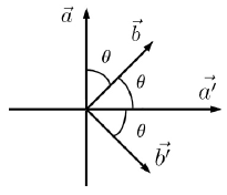
Figure 1: Schematics of the orientations for axes $\vec{a}$, $\vec{b}$, $\vec{a^{\prime}}$ and $\vec{b^{\prime}}$, where $\theta$ is the angle between a pair. Here we choose $\theta=45^{\circ}$.

III.1 Case I

In the first case, we take the model as the two quantum dots are located very close to each other and symmetrically about the antinode of the longitudinal mode sustained in the $z$ direction. Due to the symmetrical consideration we have $g_{1}=g_{2}=g$ satisfied in this case. Then we can simplify Eq. 14 as:

$$i\frac{d}{dt}C_{1}(t) = \sqrt{2}ge^{-\lambda(N_{ph}+\frac{1}{2})}e^{i(\Delta_{12}+J_{z}-\delta)t}C_{2}(t),$$

$$i\frac{d}{dt}C_{2}(t) = \sqrt{2}ge^{-\lambda(N_{ph}+\frac{1}{2})}e^{i(\Delta_{12}+J_{z}-\delta)t}C_{1}(t)$$

$$+ Ve^{-2(\lambda-\lambda_{12})(N_{ph}+\frac{1}{2})}C_{2}(t),$$

$$i\frac{d}{dt}C_{3}(t) = -Ve^{-2(\lambda-\lambda_{12})(N_{ph}+\frac{1}{2})}C_{3}(t).$$ (18)

We solve the equations above with the arbitrary initial condition

$$C_{1}(t) = e^{-i\gamma{}t/2}[\cos(\Gamma{}t/2)+i\frac{\gamma}{\Gamma}\sin(\Gamma{}t/2)]C_{1}(0)$$

$$- i\frac{2\sqrt{2}g^{\prime}}{n}[e^{-i\gamma{}t/2}\sin(\Gamma{}t/2)]C_{2}(0),$$

$$C_{2}(t) = i\frac{2\sqrt{2}g^{\prime}}{n}[e^{-\gamma{}t/2}\sin(\Gamma{}t/2)]C_{1}(0)$$

$$+ e^{-imt/2}[\cos(\Gamma{}t/2)-i\frac{\gamma}{\Gamma}\sin(\Gamma{}t/2)]C_{2}(0),$$

$$C_{3}(t) = e^{iV^{\prime}t}C_{3}(0).$$ (19)

where $C_{i}(0)$ ($i=1,2,3$) stand for the initial values of $C_{i}(t)$ at $t=0$. The parameters $g^{\prime}$, $V^{\prime}$, $\gamma$ and $\Gamma$ are given by

$$g^{\prime} = ge^{-\lambda(N_{ph}+\frac{1}{2})},$$

$$V^{\prime} = Ve^{-2(\lambda-\lambda_{12})(N_{ph}+\frac{1}{2})},$$

$$\gamma = V^{\prime}+\delta-\Delta_{12}-J_{z},$$

$$\Gamma = \sqrt{\gamma^{2}+8g^{\prime 2}}.$$ (20)

Here the generalized Rabi frequency can be defined through the parameter $\Gamma$.

Considering that the initial state of the system is a product state at $t=0$, that is: $C_{1}(0)=1$, $C_{2}(0)=C_{3}(0)=0$. With the specific choice of orientation, the Bell parameter $E(\vec{a},\vec{b})$ is given by

$$E(\vec{a},\vec{b})=|2\sqrt{2}(\frac{8g^{\prime 2}}{\Gamma^{2}})\sin^{2}(\frac{\Gamma{}t}{2})|.$$ (21)

Here we take the typical values for our DQD system: $g_{1}=g_{2}=g=1$ meV, $V=0.7$ meV, $J_{z}+\Delta_{12}=1$ meV, $\delta=2$ meV, $\lambda=0.01$ meV and $\lambda_{12}=0.005$ meV and plot an overall 3D graphic to display the trend of the Bell parameter with temperature and time in Fig. 2. Note that there is no correlation initially, but as the interaction between the cavity field and the quantum dots is turned on, the correlation develops and we do observe violation of Bell’s inequality at certain interaction times periodically. The meaning of violation of Bell’s inequality is when the curve for $E(\vec{a},\vec{b})$ lies between $2$ and $2\sqrt{2}$ (maximal quantum-mechanically allowed value). It shows that the system moves from a product state to a maximal correlated state and back again during the its time evolution. On the other hand, we notice that with the rise of the environmental temperature, the period of Bell parameter increases while the maximum of Bell parameter declines and the minimum keeps constant, shown in Fig. 3 and Fig. 4. After temperature is greater than $11.36\omega_{0}$, the maximum of Bell parameter is smaller than $2$ meaning that there is no violation of Bell’s inequality at any time. The quantum effect on the DQD system is obvious only when the temperature is very low. After an critical value of the temperature, quantum effect fades out. In order to show the relation between Bell parameter and temperature more clearly, we make the Fig. 5 at time $t=20$ ps as $E(\vec{a},\vec{b})$ oscillates and the peak decreases with the growth of temperature corresponding to the trend we have observed.

Next, we assume that the initial state of the system is a perfectly correlated state such that $|\psi(0)\rangle=|+,-,0\rangle+|-,+,0\rangle$ meaning $C_{2}(0)=1$, $C_{1}(0)=C_{3}(0)=0$ . Under this condition, the Bell parameter reads

$$E(\vec{a},\vec{b})=2\sqrt{2}|\cos^{2}(\frac{\Gamma{}t}{2})+\frac{\gamma^{2}}{\Gamma^{2}}\sin^{2}(\Gamma{}t/2)|.$$ (22)

With the same arguments of the system we used above, the 3D plot in Fig. 6 shows how Bell parameter changes with the temperature and time. Due to the entangled state initially, the Bell parameter reaches the peak $2\sqrt{2}$ at time $t=0$ ps and Bell’s inequality is violated. However, when time goes on, the violation of Bell’s inequality only appears at the certain time periodically. Concerning the temperature, both the periodic of Bell parameter in time evolution plot in Fig. 8 and the minimum of Bell parameter shown in Fig. 7 increase with the growth of the temperature while the maximum maintains just on the opposite to the last situation. Theoretically, when the temperature is greater than $130.70\omega_{0}$, the minimum of Bell parameter is always beyond $2$ and the violation of Bell’s inequality can be observed all the time.

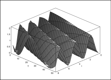
Figure 2: The plot of Bell parameter $E(\vec{a},\vec{b})$ as a function of temperature $T$ ($\omega_{0}$) and time $t$ (ps) for Case I with non-correlated initial state, for parameter $g=1$ meV, $V=0.7$ meV, $J_{z}+\Delta_{12}=1$ meV, $\delta=2$ meV, $\lambda=0.01$ and $\lambda_{12}=0.005$.

Figure 3: The plot of the maximum of Bell parameter $E$, i.e. $E(\vec{a},\vec{b})$ as a function of temperature $T$ ($\omega_{0}$) for Case I with non-correlated initial state, for parameter $g=1$ meV, $V=0.7$ meV, $J_{z}+\Delta_{12}=1$ meV, $\delta=2$ meV, $\lambda=0.01$ and $\lambda_{12}=0.005$.

Figure 4: The time evolution of Bell parameter E, i.e. $E(\vec{a},\vec{b})$ as a function of time $t$ (ps) at three different temperature for Case I with non-correlated initial state. Solid line is the result for $T=0$, dash line for $T=10\omega_{0}$ and dot line for $T=30\omega_{0}$. Here, $g=1$ meV, $V=0.7$ meV, $J_{z}+\Delta_{12}=1$ meV, $\delta=2$ meV, $\lambda=0.01$ and $\lambda_{12}=0.005$.

Figure 5: The plot of Bell parameter E, ie $E(\vec{a},\vec{b})$ as a function of temperature $T$ ($\omega_{0}$) at time $t=20$ ps for Case I with non-correlated initial state, for parameter $g=1$ meV, $V=0.7$ meV, $J_{z}+\Delta_{12}=1$ meV, $\delta=2$ meV, $\lambda=0.01$ and $\lambda_{12}=0.005$ .

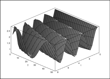
Figure 6: The plot of Bell parameter $E(\vec{a},\vec{b})$ as a function of temperature $T$ ($\omega_{0}$) and time $t$ (ps) for Case I with perfectly correlated initial state, for parameter $g=1$ meV, $V=0.7$ meV, $J_{z}+\Delta_{12}=1$ meV, $\delta=2$ meV, $\lambda=0.01$ and $\lambda_{12}=0.005$ .

Figure 7: The plot of the minimum of Bell parameter $E$, i.e. $E(\vec{a},\vec{b})$ as a function of temperature $T$ ($\omega_{0}$) for Case I with perfectly correlated initial state, for parameter $g=1$ meV, $V=0.7$ meV, $J_{z}+\Delta_{12}=1$ meV, $\delta=2$ meV, $\lambda=0.01$ and $\lambda_{12}=0.005$.

Figure 8: The time evolution of Bell parameter E, i.e. $E(\vec{a},\vec{b})$ as a function of time $t$ (ps) at three different temperature for Case I with perfectly correlated initial state. Solid line is the result for $T=0$, dash line for $T=10\omega_{0}$ and dot line for $T=30\omega_{0}$. Here, $g=1$ meV, $V=0.7$ meV, $J_{z}+\Delta_{12}=1$ meV, $\delta=2$ meV, $\lambda=0.01$ and $\lambda_{12}=0.005$.

III.2 Case II

In this case, we situate one of the quantum dot exactly one the node of the cavity-field mode while the other is quite near it, that means $g_{2}=0$ and $g_{1}\neq 0$. For this physical situation, Eq. 14 can be modified as

$$i\frac{d}{dt}C_{1}(t) = \frac{g_{1}e^{-\lambda(N_{ph}+\frac{1}{2})}}{\sqrt{2}}e^{-i(\delta-\Delta_{12}-J_{z})t}[C_{2}(t)+C_{3}(t)],$$

$$i\frac{d}{dt}C_{2}(t) = \frac{g_{1}e^{-\lambda(N_{ph}+\frac{1}{2})}}{\sqrt{2}}e^{-i(\delta-\Delta_{12}-J_{z})t}C_{1}(t)$$

$$+ Ve^{-2(\lambda-\lambda_{12})(N_{ph}+\frac{1}{2})}C_{2}(t),$$

$$i\frac{d}{dt}C_{3}(t) = \frac{g_{1}e^{-\lambda(N_{ph}+\frac{1}{2})}}{\sqrt{2}}e^{-i(\delta-\Delta_{12}-J_{z})t}C_{1}(t)$$ (23)

$$- Ve^{-2(\lambda-\lambda_{12})(N_{ph}+\frac{1}{2})}C_{2}(t).$$

The analytic solution of these equations under the condition $\delta=\Delta_{12}+J_{z}$ can be given as

$$C_{1}(t) = [\frac{V^{\prime 2}}{\Omega^{2}}+\frac{{g^{\prime}}_{1}^{2}}{\Omega^{2}}\cos(\Omega{}t)]C_{1}(0)+[\frac{{g^{\prime}}_{1}V^{\prime}}{\sqrt{2}\Omega^{2}}(\cos(\Omega{}t)-1)$$

$$- i\frac{{g^{\prime}}_{1}}{\sqrt{2}\Omega}\sin(\Omega{}t)]C_{2}(0)-[\frac{{g^{\prime}}_{1}V^{\prime}}{\sqrt{2}\Omega^{2}}(\cos(\Omega{}t)-1)$$

$$+ i\frac{{g^{\prime}}_{1}}{\sqrt{2}\Omega}\sin(\Omega{}t)]C_{3}(0)$$

$$C_{2}(t) = \frac{1}{\sqrt{2}}[\frac{{g^{\prime}}_{1}V^{\prime}}{\Omega^{2}}(\cos(\Omega{}t)-1)-i\frac{{g^{\prime}}_{1}}{\Omega}\sin(\Omega{}t)]C_{1}(0)$$

$$+ \frac{1}{2}[-i\frac{2V^{\prime}}{\Omega}\sin(\Omega{}t)+(1+\frac{{V^{\prime}}^{2}}{\Omega^{2}})(\cos(\Omega{}t)-1)$$

$$+ 2]C_{2}(0)+\frac{1}{2}[(1-\frac{{V^{\prime}}^{2}}{\Omega^{2}})(\cos(\Omega{}t)-1)]C_{3}(0),$$

$$C_{3}(t) = \frac{1}{\sqrt{2}}[-\frac{{g^{\prime}}_{1}V^{\prime}}{\Omega^{2}}(\cos(\Omega{}t)-1)-i\frac{{g^{\prime}}_{1}}{\Omega}\sin(\Omega{}t)]C_{1}(0)$$ (24)

$$+ \frac{1}{2}[(1-\frac{{V^{\prime}}^{2}}{\Omega^{2}})(\cos(\Omega{}t)-1)]C_{2}(0)+\frac{1}{2}[i\frac{2V^{\prime}}{\Omega}\sin(\Omega{}t)$$

$$+ (1+\frac{{V^{\prime}}^{2}}{\Omega^{2}})(\cos(\Omega{}t)-1)+2]C_{3}(0).$$

where

$${g^{\prime}}_{1} = g_{1}e^{-\lambda(N_{ph}+\frac{1}{2})},$$

$$\Omega^{2} = {g^{\prime}}_{1}^{2}+{V^{\prime}}^{2}.$$ (25)

Here $\Omega$ is the generalized Rabi frequency.

When both of the quantum dots are in their ground state initially, ie $C_{1}(0)=1$, $C_{2}(0)=C_{3}(0)=0$, since the initial state of the system is a product state and the second quantum dot sitting on the node does not interact with the cavity field, the system never goes to the correlated state and we can not find the violation of Bell’s equality for the entire time evolution at any temperature including zero temperature. However, if the two quantum dots are initially perfectly correlated, with the arguments $C_{2}(0)=1$ and $C_{1}(0)=C_{3}(0)=0$, we have Bell parameter as

$$E(\vec{a},\vec{b})=2\sqrt{2}|\cos(\Omega{}t)+\frac{{V^{\prime}}^{2}}{\Omega}(1-\cos(\Omega{}t))|.$$ (26)

In Fig. 9, an 3D plot of $E(\vec{a},\vec{b})$ as function of time and temperature is shown. The maximum of Bell parameter keeps the same at the value of $2\sqrt{2}$ in the time evolution plot. However, the minimum maintain zero until that temperature reaches $40.88\omega_{0}$ and the DQD system shows up at product state, i.e. $E(\vec{a},\vec{b})=0$, at certain time points periodically. After that critical point, the minimum of Bell parameter rises dramatically with the growth of temperature and our DQD system is always in the correlated state. Surprisingly, when temperature is higher than $75.54\omega_{0}$, shown in Fig. 10, the Bell parameter will be greater than the maximal value which quantum-mechanically allowed. Since the approximation of the omission of nondiagonal transition in Eq.  1 can be used at low temperature, it implies that when temperature is greater than $75.54\omega_{0}$, the approximation is no longer suitable for this theoretical model. In Fig. 11, we draw the time evolution plot of Bell parameter at four temperature, especially at $T=50\omega_{0}$, to explicit the system without the product state during its evolution time.

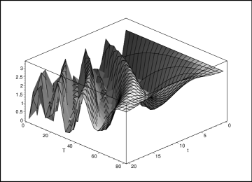
Figure 9: The plot of Bell parameter $E(\vec{a},\vec{b})$ as a function of temperature $T$ ($\omega_{0}$) and time $t$ (ps) for Case II with non-correlated initial state, for parameter $g_{1}=1$ meV, $g_{2}=0$ mV, $V=0.7$ meV, $J_{z}+\Delta_{12}=1$ meV, $\delta=2$ meV, $\lambda=0.01$ and $\lambda_{12}=0.005$.

Figure 10: The plot of the minimum of Bell parameter $E$, i.e. $E(\vec{a},\vec{b})$ as a function of temperature $T$ ($\omega_{0}$) for Case II with non-correlated initial state, for parameter $g_{1}=1$ meV, $g_{2}=0$ mV, $V=0.7$ meV, $J_{z}+\Delta_{12}=1$ meV, $\delta=2$ meV, $\lambda=0.01$ and $\lambda_{12}=0.005$.

Figure 11: The time evolution of Bell parameter E, i.e. $E(\vec{a},\vec{b})$ as a function of time $t$ (ps) at three different temperature for Case II with non-correlated initial state. Solid line is the result for $T=0$, dash line for $T=10\omega_{0}$ and dot line for $T=30\omega_{0}$. Here, $g=1$ meV, $V=0.7$ meV, $J_{z}+\Delta_{12}=1$ meV, $\delta=2$ meV, $\lambda=0.01$ and $\lambda_{12}=0.005$.

III.3 Case III

Finally, we consider a general situation where the two quantum dots are situated in the cavity such that they are affected by the field differently, ie $g_{1}\neq{}g_{2}$ and both $g_{1}$, $g_{2}>0$. In order to obtain an analytic solution, we simplify the model by assuming that the separation of the quantum dots is large enough so that the Förster interaction between them becomes very weak in comparison to the exciton-cavity-field interaction and can be neglected. Hence the Eq. 14 changes to

$$i\frac{d}{dt}C_{1}(t) = \frac{1}{\sqrt{2}}e^{-i(\delta-\Delta_{12}-J_{z})t}[(g_{1}e^{-\lambda(N_{ph}+\frac{1}{2})}$$

$$+ g_{2}e^{-\lambda(N_{ph}+\frac{1}{2})})C_{2}(t)+(g_{1}e^{-\lambda(N_{ph}+\frac{1}{2})}$$

$$- g_{2}e^{-\lambda(N_{ph}+\frac{1}{2})})C_{3}(t)],$$

$$i\frac{d}{dt}C_{2}(t) = \frac{1}{\sqrt{2}}e^{-i(\delta-\Delta_{12}-J_{z})t}(g_{1}e^{-\lambda(N_{ph}+\frac{1}{2})}$$

$$+ g_{2}e^{-\lambda(N_{ph}+\frac{1}{2})})C_{1}(t),$$

$$i\frac{d}{dt}C_{3}(t) = \frac{1}{\sqrt{2}}e^{-i(\delta-\Delta_{12}-J_{z})t}(g_{1}e^{-\lambda(N_{ph}+\frac{1}{2})}$$ (27)

$$- g_{2}e^{-\lambda(N_{ph}+\frac{1}{2})})C_{1}(t).$$

The analytic solution of the equations above reads

$$C_{1}(t) = e^{-i\xi{}t/2}[\cos(\frac{\Xi{}t}{2})+i\frac{\xi}{\Xi}\sin(\frac{\Xi{}t}{2})]C_{1}(0)$$

$$- i\frac{\sqrt{2}({g^{\prime}}_{1}+{g^{\prime}}_{2})}{\Xi}e^{-i\xi{}t/2}\sin(\frac{\Xi{}t}{2})C_{2}(0)$$

$$- i\frac{\sqrt{2}({g^{\prime}}_{1}-{g^{\prime}}_{2})}{\Xi}e^{-i\xi{}t/2}\sin(\frac{\Xi{}t}{2})C_{3}(0),$$

$$C_{2}(t) = -i\frac{\sqrt{2}({g^{\prime}}_{1}+{g^{\prime}}_{2})}{\Xi}e^{i\xi{t}/2}\sin(\frac{\Xi{}t}{2})C_{1}(0)$$

$$+ \{\frac{({g^{\prime}}_{1}+{g^{\prime}}_{2})^{2}}{2({g^{\prime}}_{1}^{2}+{g^{\prime}}_{2}^{2})}e^{-i\xi{}t/2}[\cos(\frac{\Xi{}t}{2})-i\frac{\xi}{\Xi}\sin(\frac{\Xi{}t}{2})]$$

$$+ \frac{({g^{\prime}}_{1}-{g^{\prime}}_{2})^{2}}{2({g^{\prime}}_{1}^{2}+{g^{\prime}}_{2}^{2})}\}C_{2}(0)$$

$$+ \{\frac{({g^{\prime}}_{1}^{2}-{g^{\prime}}_{2}^{2})}{2({g^{\prime}}_{1}^{2}+{g^{\prime}}_{2}^{2})}e^{-i\xi{}t/2}[\cos(\frac{\Xi{}t}{2})-i\frac{\xi}{\Xi}\sin(\frac{\Xi{}t}{2})]$$

$$- \frac{({g^{\prime}}_{1}^{2}-{g^{\prime}}_{2}^{2})}{2({g^{\prime}}_{1}^{2}+{g^{\prime}}_{2}^{2})}\}C_{3}(0)$$

$$C_{3}(t) = -i\frac{\sqrt{2}({g^{\prime}}_{1}-{g^{\prime}}_{2})}{\Xi}e^{i\xi{t}/2}\sin(\frac{\Xi{}t}{2})C_{1}(0)$$ (28)

$$+ \{\frac{({g^{\prime}}_{1}^{2}-{g^{\prime}}_{2}^{2})}{2({g^{\prime}}_{1}^{2}+{g^{\prime}}_{2}^{2})}e^{-i\xi{}t/2}[\cos(\frac{\Xi{}t}{2})-i\frac{\xi}{\Xi}\sin(\frac{\Xi{}t}{2})]$$

$$- \frac{({g^{\prime}}_{1}^{2}-{g^{\prime}}_{2}^{2})}{2({g^{\prime}}_{1}^{2}+{g^{\prime}}_{2}^{2})}\}C_{2}(0)$$

$$+ \{\frac{({g^{\prime}}_{1}+{g^{\prime}}_{2})^{2}}{2({g^{\prime}}_{1}^{2}+{g^{\prime}}_{2}^{2})}e^{-i\xi{}t/2}[\cos(\frac{\Xi{}t}{2})-i\frac{\xi}{\Xi}\sin(\frac{\Xi{}t}{2})]$$

$$+ \frac{({g^{\prime}}_{1}+{g^{\prime}}_{2})^{2}}{2({g^{\prime}}_{1}^{2}+{g^{\prime}}_{2}^{2})}\}C_{3}(0)$$

where

$${g^{\prime}}_{2} = g_{2}e^{-\lambda(N_{ph}+\frac{1}{2})},$$

$$\xi = \delta-\Delta_{12}-J_{z},$$

$$\Xi = \sqrt{\xi^{2}+4({g^{\prime}}_{1}^{2}+{g^{\prime}}_{2}^{2})}.$$ (29)

When the two quantum dots are in the ground states initially, we take the value $C_{1}(0)=1$, $C_{2}(0)=C_{3}(0)=0$, for Bell parameter,

$$E(\vec{a},\vec{b})=4\sqrt{2}|\frac{({g^{\prime}}_{1}+{g^{\prime}}_{2})^{2}-({g^{\prime}}_{1}-{g^{\prime}}_{2})^{2}}{\Xi^{2}}\sin^{2}(\frac{\Xi{}t}{2})|.$$ (30)

For an general situation that two quantum dots are located differently in the field, we use the arguments that $g_{1}=1$ meV and $g_{2}=0.7$ meV. The other arguments of the system reads: $V=0.7$ meV, $J_{z}+\Delta_{12}=1$ meV, $\delta=2$ meV, $\lambda=0.01$ and $\lambda_{12}=0.005$, just the same as in Case I. For this condition, $E(\vec{a},\vec{b})$ is plot in Fig 12 as function of time and temperature. As we note, the maximum of Bell parameter in time evolution in Fig 13, 14, rises. However, when the temperature is higher than $33.63\omega_{0}$, Bell the maximum is smaller than $2$, meaning that Bell inequality will no longer be violated. Such value is about triple as that we got in Case I.

Lastly, we discuss the situation that $E(\vec{a},\vec{b})$ in time evolution begins with perfectly correlated state and the probability amplitude reads as $C_{2}(0)=1$, $C_{1}(0)=C_{3}(0)=0$,

$$E(\vec{a},\vec{b}) = \frac{2\sqrt{2}}{4({g^{\prime}}_{1}^{2}+{g^{\prime}}_{2}^{2})}|[\cos^{2}(\frac{\Xi{}t}{2})+(\frac{\xi}{Xi})^{2}\sin^{2}(\frac{\Xi{}t}{2})]$$ (31)

$$\times [({g^{\prime}}_{1}+{g^{\prime}}_{2})^{4}-({g^{\prime}}_{1}^{2}-{g^{\prime}}_{2}^{2})^{2}]$$

$$+ [({g^{\prime}}_{1}-{g^{\prime}}_{2})^{4}-({g^{\prime}}_{1}^{2}+{g^{\prime}}_{2}^{2})^{2}]+4({g^{\prime}}_{1}^{2}-{g^{\prime}}_{2}^{2})^{2}$$

$$\times [\cos(\frac{\Xi{}t}{2})\cos(\frac{\xi{}t}{2})+\frac{\xi}{\Xi}\sin(\frac{\Xi{}t}{2})\sin(\frac{\xi{}t}{2})]|.$$

As we can see in 3D plot in Fig 15, Bell parameter begins the time evolution with the value of $2\sqrt{2}$, ie perfectly correlated. When the temperature is low enough, the DQD system will never be unentangled to the product state during the time evolution. The minimum of $E(\vec{a},\vec{b})$ in time evolution plot in Fig 16 is smaller than $2$, i.e. there is violation of Bell’s inequality only periodically.

Figure 12: The plot of Bell parameter $E(\vec{a},\vec{b})$ as a function of temperature $T$ ($\omega_{0}$) and time $t$ (ps) without Föster interaction for Case III with non-correlated initial state, for parameter $g_{1}=1$, $g_{2}=0.7$ meV, $V=0.7$ meV, $J_{z}+\Delta_{12}=1$ meV, $\delta=2$ meV, $\lambda=0.01$ and $\lambda_{12}=0.005$.

Figure 13: The plot of the maximum of Bell parameter $E$, i.e. $E(\vec{a},\vec{b})$ as a function of temperature $T$ ($\omega_{0}$) without Föster interaction for Case III with non-correlated initial state, for parameter $g_{1}=1$, $g_{2}=0.7$ meV, $V=0.7$ meV, $J_{z}+\Delta_{12}=1$ meV, $\delta=2$ meV, $\lambda=0.01$ and $\lambda_{12}=0.005$.

Figure 14: The time evolution of Bell parameter E, i.e. $E(\vec{a},\vec{b})$ as a function of time $t$ (ps) without Föster interaction at three different temperature for Case III with non-correlated initial state. Solid line is the result for $T=0$, dash line for $T=10\omega_{0}$ and dot line for $T=30\omega_{0}$. Here, $g_{1}=1$, $g_{2}=0.7$ meV, $V=0.7$ meV, $J_{z}+\Delta_{12}=1$ meV, $\delta=2$ meV, $\lambda=0.01$ and $\lambda_{12}=0.005$.

Figure 15: The plot of Bell parameter $E(\vec{a},\vec{b})$ as a function of temperature $T$ ($\omega_{0}$) and time $t$ (ps) without Föster interaction for Case III with perfectly correlated initial state, for parameter $g_{1}=1$, $g_{2}=0.7$ meV, $V=0.7$ meV, $J_{z}+\Delta_{12}=1$ meV, $\delta=2$ meV, $\lambda=0.01$ and $\lambda_{12}=0.005$.

Figure 16: The time evolution of Bell parameter E, i.e. $E(\vec{a},\vec{b})$ as a function of time $t$ (ps) without Föster interaction at three different temperature for Case III with perfectly correlated initial state. Solid line is the result for $T=0$, dash line for $T=10\omega_{0}$ and dot line for $T=30\omega_{0}$. Here, $g_{1}=1$, $g_{2}=0.7$ meV, $V=0.7$ meV, $J_{z}+\Delta_{12}=1$ meV, $\delta=2$ meV, $\lambda=0.01$ and $\lambda_{12}=0.005$.

IV Conclusion

In summary, we have investigated a double quantum dot system with exciton-phonon interaction and Förster interaction at finite environmental temperature. As the time evolution of Wootters’ measure, which is used to quantify the entanglement of bipartite system, is in excellent agreement with the time evolution of Bell’s equality Hill ; Joshi ; Wootters , we used violation of CHSH inequality as a tool to look into the entanglement of two quantum dots system at finite temperature. Concerning the location of the two quantum dots in the microcavity, we have discussed our theoretical model in three situations with different initial states. When the system starts with the product state, both of the quantum dots stay in the ground state, the violation of Bell’s inequality in Case I and III becomes weaker with the rise of the temperature and after the temperature is high enough, it fades out, while in Case II the violation of Bell’s inequality has never been found in the whole time evolution. The quantum effect in our DQD system becomes weaker and weaker with the growth of temperature and disappears when the temperature is high enough. On the other hand, since the Bell’s parameter is a kind of indictor of the entanglement of the system, from our time evolution pictures we can conclude: as the DQD system begins its time evolution with non-correlated state, the higher the temperature, the weaker the periodical entanglement. However, when the two coupled quantum dots system is perfectly correlated initially, as the temperature grows, the periodical entanglement of the system become stronger. Nevertheless, in Case II, when the temperature is too high, the Bell parameter rises beyond the quantum-mechanical allowed value and our DQD model is no longer suitable for such research.

V Acknowledgments

This work has been supported in part by National Natural Science Foundation of China and the National Minister of Education Program for Changjiang Scholars and Innovative Research Team in University (PCSIRT).

References

- (1) G. Benenti, G. Casati, and G. Strini, Principles of Quantum Computation and Information (World Scientific, Singapore, 2004), Vol.I.
- (2) M. A. Nielsen and I. L. Chuang, Quantum Computation and Quantum Information (Cambridge University Press, Cambridge, U. K., 2000).
- (3) D. Bouwmeester, A. K. Ekert, and A. Zeilinger, The Physics of Quantum Information (Springer-Verlag, Berlin, 2000).
- (4) D. Gammon, E. S. Snow, B.V.Shanabrook, D. S. Katzer, and D. Park, Science 273, 87 (1996);
- (5) X. Li, Y. W. Wu, D. Steel, D. Gammon, T. H. Stievater, D. S. Katzer, D. Park, C. Piermarocchi, and L. J. Sham, Science 301, 809 (2003);
- (6) P. Bianucci, A. Muller, C. K. Shih, Q. Q. Wang, Q. K. Xue, and C. Piermarocchi, Phys. Rev. B 69, 161303(R) (2004).
- (7) N. H. Bonadeo, J. Erland, D. Gammon, D. Park, D. S. Katzer, and D.G. Steel, Science 282, 1473 (1998).
- (8) P.M. Petroff, A. Lorke, and A. Imamoğlu, Phys. Today 54, 46 (2001).
- (9) O.B. Shchekin, G. Park, D.L. Huffaker, and D.G. Deppe, Appl. Phys. Lett. 77, 466 (2000).
- (10) H. Saito, K. Nishi, and S. Sugou, Appl. Phys. Lett. 78, 267 (2001)
- (11) A. Zrenner, E. Beham, S. Stufler, F. Fndeis, M. Bichler, G. Abstreiter, Nature 418, 612 (2002).
- (12) E. Biolatti, R. C. Lotti, P. Zanardi, and F. Rossi, Phys. Rev. Lett. 85, 5647 (2000).
- (13) A. Imamoğlu, D. D. Awschalom, G. Burkard, D. P. DiVincenzo, D. Loss, M. Sherwin, and A. Small, Phys. Rev. Lett. 83, 4204 (1999).
- (14) D. Loss and D. P. DiVincenzo, Phys. Rev. A 57, 120 (1998).
- (15) T. Pellizzari, S. A. Gardiner, J. I. Cirac, and P. Zoller, Phys. Rev. Lett. 75, 3788 (1995).
- (16) L. Besombes, K. Kheng, L. Marsal, and H. Mariette, Phys. Rev. B 63, 155307 (2001).
- (17) R. Heitz, I. Mukhametzhanov, O. Stier, A. Madhukar, and D. Bimberg, Phys. Rev. Lett. 83, 4654 (1999).
- (18) S. Hameau, Y. Guldner, O. Verzelen, R. Ferreira, G. Bastard, J. Zeman, A. Lemaitre, and J. M. Gerard, Phys. Rev. Lett. 83, 4152 (1999).
- (19) X.Z. Yuan, K.D. Zhu, and W.S. Li, Phys. Lett. A 329, 402 (2004).
- (20) L. Quiroga and N. F. Johnson, Phys. Rev. Lett. 83, 2270 (1999).
- (21) B. W. Lovett, J. H. Reina, A. Nazir, B. Kothari, and G. A. D. Briggs, Phys. Lett. A 315, 136 (2003).
- (22) A. Nazir, B. W. Lovett, S. D. Barrett, J. H. Reina, and G. A. D. Briggs, quant-ph/0309099.
- (23) J. H. Reina, L. Quiroga, N. F. Johnson, Phys. Rev. A. 62, 012305 (2000).
- (24) J. H. Reina and N. F. Johnson, Phys. Rev. A. 63, 012303 (2000).
- (25) I. Wilson-Rae and A. Imamoǧlu, Phys. Rev. B 65, 235311 (2002).
- (26) K.D. Zhu and W.S. Li, Phys. Lett. A 314, 380 (2003).
- (27) Y. X. Liu, S. K. Özdemir, M. Koashi, and N. Imoto, Phys. Rev. A 65, 042326 (2002).
- (28) G. X. Li, Y. P. Yang, K. Allaart, and D. Lenstra, Phys. Rev. A 69, 014301 (2004).
- (29) G. X. Li, H. T. Tan, S. P. Wu, and Y. P. Yang, Phys. Rev. A 70, 034307 (2004).
- (30) J. F. Clauser, M. A. Horne, A. Shimony, and R. A. Holt, Phys. Rev. Lett. 23, 880 (1969).
- (31) J. F. Clauser and A. Shimony, Rep. Prog. Phys. 41, 1881 (1978).
- (32) A. Joshi, B. Anderson, and M. Xiao, Phys. Rev. B 75, 125304 (2007).
- (33) S. Gröblacher, T. Paterek, R. Kaltenbaek, Ĉ. Brukner, M. Żukowski, M. Aspelmeyer, and A. Zeilinger, Nature 446, 05677 (2007).
- (34) G. Oohata, R. Shimizu, and K. Edamatsu, Phys. Rev. Lett. 98, 140503 (2007).
- (35) T. Förster, Disc. Farad. Soc. 27, 7 (1959).
- (36) I.V. Bondarev, S.A. Madsimenko, and G.Ya. Slepyan, Phys. Rev. B 68, 073310 (2003).
- (37) S.De Rinaldis, I. D’Amico, E. Biolatti, R. Rinaldi, R. Cingolani, and F. Rossi, Phys. Rev. B 65 081309 (2002).
- (38) Xiao-Zhong Yuan and Ka-Di Zhu, Phys. Rev. B 74, 073309 (2006).
- (39) G. D. Mahan, Many-Particle Physics (Plenum, New York, 2000).
- (40) Z. Z. Chen, R. Lu, and B. F. Zhu, Phys. Rev. B 71, 165324 (2005).
- (41) T. Brandes and B. Kramer, Phys. Rev. Lett. 83, 3021 (1999).
- (42) N. H. Bonadeo, Gang Chen, D. Gammon, D. S. Katzer, D. Park, and D. G. Steel, Phys. Rev. Lett. 81, 2759 (1998).
- (43) J. P. Reithmaier, G. Sek, A. Löffler, C. Hofmann, S. Kuhn, S. Reitzenstein, L. V. Keldysh, V. D. Kulakovskii, T. L. Reinecke, and A. Forchel, Nature 432, 197 (2004).
- (44) A. Einstein, B, Pdodolskty, and N. Rosen, Phys. Rev. 47, 777 (1935).
- (45) J. Bell, Phys. I, 195 (1964).
- (46) J. Bell, Rev. Mod. Phys. 38,447 (1966).
- (47) A. Aspect, P. Grangier, and G. Roger, Phys. Rev. Lett. 49, 91 (1982).
- (48) S. Hill and W. K. Wootters, Phys. Rev. Lett. 78, 5022 (1997).
- (49) W. K. Wootters, Phys. Rev. Lett. 80, 2245 (1998).