Efficient ab initio calculations of bound and continuum excitons

Abstract

We present calculations of the absorption spectrum of semiconductors and insulators comparing various approaches: (i) the two-particle Bethe-Salpeter equation of Many-Body Perturbation Theory; (ii) time-dependent density-functional theory using a recently developed kernel that was derived from the Bethe-Salpeter equation; (iii) a scheme that we propose in the present work and that allows one to derive different parameter-free approximations to (ii). We show that all methods reproduce the series of bound excitons in the gap of solid argon, as well as continuum excitons in semiconductors. This is even true for the simplest static approximation, which allows us to reformulate the equations in a way such that the scaling of the calculations with number of atoms equals the one of the Random Phase Approximation.

Time-dependent density-functional theory (TDDFT) runge is more and more considered to be a promising approach for the calculation of neutral electronic excitations, even in extended systems onida ; tddftbook . In linear response, spectra are described by the Kohn-Sham independent-particle polarizability $\chi_{0}^{\tiny{KS}}$ and the frequency-dependent exchange-correlation (xc) kernel $f_{xc}$. The widely used adiabatic local-density approximation zangwill ; gross (TDLDA), with its static and short-ranged kernel, often yields good results in clusters but fails for absorption spectra of solids. Instead, more sophisticated approaches derived from Many-Body Perturbation Theory (MBPT) reining ; sottile ; adragna ; marini ; stubner have been able to reproduce, ab initio, the effect of the electron-hole interaction in extended systems, not least thanks to an explicit long-range contribution deboeij ; reining ; botti . The latter strongly influences spectra like optical absorption or energy loss, especially for relatively small momentum transfer.

Here we show that this kernel is even able to reproduce the hydrogen-like excitonic series in the photoemission gap of a rare gas solid. However the kernel has a strong spatial and frequency dependence, and its evaluation requires a significant amount of computer time. We therefore tackle the question of a parameter-free, but quick TDDFT calculation of excitonic effects in solids, which has been so far an unsolved problem, and show that a much more efficient formulation can indeed be achieved. In particular we demonstrate how it is possible for a wide range of materials to obtain good absorption spectra including excitonic effects with a static kernel leading in principle to a Random Phase Approximation (RPA)-like scaling of the calculation with the number of atoms of the system.

Atomic units are used throughout the paper. The vectorial character of the quantities $r,k,G,q$ (where $k$ and $q$ are vectors in the Brillouin zone, and $G$ is a reciprocal lattice vector) is implicit. Only transitions of positive frequency (i.e. resonant contributions), which dominate absorption spectra, are considered throughout.

Let us first concentrate on the absorption spectrum of solid argon. The low band dispersion, together with the small polarizability of the solid, conjures a picture where the electron-hole interaction is very strong and gives rise to a whole series of bound excitons below the interband threshold. As in the optical spectra of other rare gas solids, the first exciton is strongly bound (in argon by $\sim 2$ eV), falling in the class of localized Frenkel frenkel excitons. Closer to the continuum onset at 14.2 eV, one finds more weakly bound Mott-Wannier wannier type excitons in a hydrogen-like series. In the ab initio framework, such a complex spectrum is typically described by the solution of the four-point (electron-hole) Bethe-Salpeter equation (BSE) hanke ; strinati ; onida . In Fig.1 we show the optical spectrum of solid argon calculated within the BSE approach, and within TDDFT both using TDLDA details and the MBPT-derived kernel sottile . The agreement of the BSE curve with experiment (line-circles) argonexp (and with previous BSE calculations patterson ) is good, concerning both position and relative intensity of the first two peaks. It should be noted that the experiment shows double peaks due to spin-orbit splitting, which is not taken into account in our calculations. The latter yields the singlet excitons that should essentially relate to the hole with $j=1/2$ and be compared with the $n^{\prime}$ peaks. Besides the spin-orbit splitting, the pseudopotential approximation as well as the construction of a static $W$ from LDA ingredients contribute to the remaining discrepancy with experiment. In spite of these limitations, the $n^{\prime}=3$ peak can also be detected, although the 2048 k-points used to calculate the spectrum are not sufficient to discuss it quantitatively, nor to describe the higher peaks. Instead, the first two peaks require less k-points and, as can be seen in the inset, are already well reproduced with 256 k-points. In the following we therefore concentrate on these two structures and perform all calculations with 256 k-points.

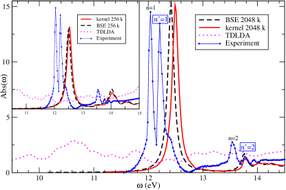
Figure 1: Absorption spectrum of solid Ar. The BSE (dashed) and TDDFT using kernel of Ref. sottile (solid) are compared (only the $n^{\prime}$ singlet exciton series) with experiment argonexp . TDLDA is given by the points. Main panel: calculation with 2048 k-points. Inset: 256 k-points

The BSE impressively improves upon the TDLDA (dotted), which shows a structure-less broad curve, clearly missing the bound excitons. Instead, the kernel of Ref. sottile (full curve in Fig. 1) leads to the same accuracy as the BSE, both for the Frenkel exciton and for the following structures. This demonstrates the potential of the method and shows that the MBPT-derived kernel can be used to quantitatively predict the absorption spectra of a wide range of materials, including the insulating rare-gas solids.

However, the method is still computationally relatively heavy. Indeed in the MBPT-derived TDDFT approach, right as for the BSE two-particle Hamiltonian, one has to evaluate the matrix elements $F_{tt^{\prime}}^{\text{\tiny{BSE}}}$ of the statically screened electron-hole Coulomb interaction $W$,

$$F_{tt^{\prime}}^{\text{\tiny{BSE}}}\!=\!-2\pi\alpha\!\!\int\!\!dr_{1}dr_{2}\,\tilde{\Phi}^{*}_{t}(r_{1},r_{2})W(r_{1},r_{2})\tilde{\Phi}_{t^{\prime}}(r_{1},r_{2})$$ (1)

where the product $\tilde{\Phi}_{t}(r_{1},r_{2})=\phi_{vk}(r_{1})\phi^{*}_{ck+q}(r_{2})$ of two KS wavefunctions $\phi$ is a generalized non local transition term; here $t$ is an index of transition with momentum transfer $q$, i.e. $t=\{vckq\}$, from valence $vk$ to conduction $ck+q$ states. $\alpha=2/(N_{k}\Omega_{0})$ with $N_{k}$ number of k-points and $\Omega_{0}$ volume of the unit cell. The calculation of $F_{tt^{\prime}}^{\text{\tiny{BSE}}}$ scales with the number of atoms $N_{at}$ as $N_{r}N_{t}^{2}\sim N_{at}^{5}$, where $N_{r}$ is the number of points in real space, and $N_{t}$ is the total number of transitions. Following Ref. sottile , one then constructs an approximate kernel $f_{xc}^{\text{eff},{\mathcal{A}}}=\chi_{0}^{-1}T^{\text{eff}}_{\mathcal{A}}\chi_{0}^{-1}$ with

$$T^{\text{eff}}_{\mathcal{A}}(r,r^{\prime},\omega)\!=\!\alpha\!\sum_{tt^{\prime}}\!\frac{\Phi_{t}(r)}{(\omega+i\eta-\!\Delta E_{t})}F^{\text{\tiny{BSE}}}_{tt^{\prime}}\frac{\Phi_{t^{\prime}}^{*}(r^{\prime})}{(\omega+i\eta-\!\Delta E_{t^{\prime}})}$$

where $\Phi_{t}(r_{1})=\tilde{\Phi}_{t}(r_{1},r_{1})$ and $\Delta E_{t}$ are differences between quasi-particle (QP) eigenvalues, since $f_{xc}^{\text{eff},{\mathcal{A}}}$ is an approximation to the “many-body” kernel $f_{xc}^{\text{mb}}$ that has to be used in conjunction with an independent particle response function $\chi_{0}$ built with QP energies instead of Kohn-Sham (KS) ones as in pure TDDFT. This kernel simulates hence to good approximation the electron-hole interaction that is described by the BSE sottile .

Even though this construction can be optimized marini the method is at least an order of magnitude slower than an RPA calculation. In the following we show how this problem can be overcome.

We concentrate on the irreducible polarizability $P$ that yields via the bare Coulomb interaction $v$ the reducible polarizability $\chi$ from the matrix equation $\chi=P+Pv\chi$, and the inverse dielectric matrix $\epsilon^{-1}=1+v\chi$. All quantities are functions of $q$ and frequency $\omega$, and matrices in $G,G^{\prime}$. Absorption spectra are then obtained from $\text{Abs}(\omega)=\displaystyle\lim_{q\to 0}\text{Im}\left\{1/\epsilon_{00}^{-1}(q,\omega)\right\}$. The polarizability $P$ is determined from the screening equation $P=\chi_{0}+\chi_{0}f_{xc}^{\text{mb}}P$. In this equation we can now insert to the left and right of $f_{xc}^{\text{mb}}$ the identity $1=XX^{-1}=X^{-1}X$, providing that $X$ is a non-singular function. This yields

$$P=\chi_{0}+\chi_{0}X^{-1}TX^{-1}P$$ (2)

where $T=Xf_{xc}^{\text{mb}}X$. We choose a matrix of the form $X=\alpha\sum_{t}g_{t}(\omega)\Phi_{t}(r)\Phi_{t}^{*}(r^{\prime})$, where $g_{t}(\omega)$ is an arbitrary function. The term $T$ contains an explicit sum over matrix elements $F^{\text{\tiny{TDDFT}}}_{tt^{\prime}}=4\pi\alpha\int dr_{1}\,dr_{2}\,\Phi_{t}^{*}(r_{1})f_{xc}^{\text{mb}}(r_{1},r_{2},\omega)\Phi_{t}(r_{2})$ in a basis of transitions $\Phi_{t}$, namely

$$T(r,r^{\prime},\omega)\!=\!\alpha\sum_{tt^{\prime}}g_{t}(\omega)\Phi_{t}(r)F^{\text{\tiny{TDDFT}}}_{tt^{\prime}}g_{t^{\prime}}(\omega)\Phi_{t^{\prime}}^{*}(r^{\prime}).$$ (3)

The exact $F^{\text{\tiny{TDDFT}}}_{tt^{\prime}}$ is of course not known. However, in the spirit of Refs. sottile ; reining we now replace the unknown matrix elements $F^{\text{\tiny{TDDFT}}}_{tt^{\prime}}$ with the BSE ones, given by Eq.(1). With this mapping, $T$ is approximated as

$$T\longrightarrow T^{\text{eff}}=\alpha\sum_{tt^{\prime}}g_{t}(\omega)\Phi_{t}(r)\left[\int dr_{1}\,dr_{2}\,\tilde{\Phi}_{t}^{*}(r_{1},r_{2})W(r_{1},r_{2})\tilde{\Phi}_{t^{\prime}}(r_{1},r_{2})\right]\Phi_{t^{\prime}}^{*}(r^{\prime})g_{t^{\prime}}(\omega)=\;X^{3}W\;^{3}\!X$$ (4)

where we have defined a three-point right and left $X$ operator as: $X^{3}(r_{1};r_{2}r_{2^{\prime}};\omega)=\alpha\sum_{t}g_{t}(\omega)\Phi_{t}(r_{1})\tilde{\Phi}_{t}^{*}(r_{2},r_{2^{\prime}})$ and ${}^{3}\!X(r_{1}r_{1^{\prime}};r_{2};\omega)=\alpha\sum_{t}g_{t}(\omega)\tilde{\Phi}_{t^{\prime}}(r_{1},r_{1^{\prime}})\Phi_{t^{\prime}}^{*}(r_{2})$. Here it is important to underline that $F^{\text{\tiny{TDDFT}}}_{tt^{\prime}}$ are constructed as matrix elements of the local $\Phi_{t}(r)$, whereas $F_{tt^{\prime}}^{\text{\tiny{BSE}}}$ are matrix element of the non-local $\tilde{\Phi}_{t}(r,r^{\prime})$. In fact the mapping (4) is not an exact operation, because $F_{tt^{\prime}}^{\text{\tiny{BSE}}}$ cannot be expressed as a matrix element (between $\Phi_{t}$ and $\Phi_{t^{\prime}}$) of a single $f_{xc}^{\text{mb}}$ for all $t,t^{\prime}$ sottile ; reining ; sottile3 . Therefore $f_{xc}^{\text{eff}}=X^{-1}T^{\text{eff}}X^{-1}$ can be different from $f_{xc}^{\text{mb}}$, and the quality of the resulting spectra will depend on the choice of $X$.

If a certain freedom in the choice of $g_{t}$ can be exploited, one may find approaches that boost the computational efficiency with respect to $f_{xc}^{\text{eff},\mathcal{A}}$, i.e. the expression of sottile .

In the following we will first illustrate, with the example of bulk Silicon and solid Argon, how different choices for $g_{t}(\omega)$ can lead to very similar spectra.

We label with calligraphic letters the different choices $\mathcal{A,B,C,D}$ that stand for:

$$\begin{split}{\mathcal{A}})\quad g_{t}(\omega)&=1/\left(\omega-\Delta E_{t}+i\eta\right),\quad\textrm{(i.e}\quad X=\chi_{0}\textrm{)}\\ {\mathcal{B}})\quad g_{t}(\omega)&=\text{Im}\left\{1/\left(\omega-\Delta E_{t}+i\eta\right)\right\}\\ {\mathcal{C}})\quad g_{t}(\omega)&=1/\Delta E_{t}\qquad;\qquad{\mathcal{D}})\quad g_{t}(\omega)=1\end{split}$$ (5)

The first choice (${\mathcal{A}}$) defines nothing but the case $X=\chi_{0}$, as proposed in Ref. sottile and leading to $f_{xc}^{\text{eff},{\mathcal{A}}}$ above; in the second case (${\mathcal{B}}$) only the imaginary part is taken from the denominator of the independent particle polarizability (very localized function in frequency); the cases (${\mathcal{C}}$) and (${\mathcal{D}}$) describe simple static choices for $g_{t}(\omega)$.

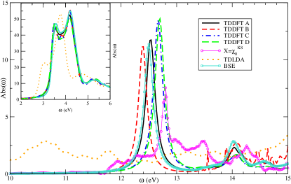
Figure 2: Main: illustration of the different choices for Eq.(5). In the inset: same choices for the absorption spectrum of Si.

The inset of Fig.2 shows the optical absorption of bulk Silicon calculated with the BSE and within TDDFT, using these mapping kernels ($\mathcal{A,B,C,D}$); the TDLDA result is also shown in order to emphasize the little differencies among the mapping kernels, compared to the huge improvements of ($\mathcal{A,B,C,D}$) with respect to TDLDA. The description of the optical absorption of Argon is a much more stringent test. In Fig.2 we see that all the different kernels ($\mathcal{A}$ being slightly better than the others) are able to well reproduce the excitonic series and to strongly improve upon the TDLDA result (dotted curve). This is especially surprising for choices ($\mathcal{C}$) and ($\mathcal{D}$): bound excitons have up to now only been obtained using either the full, strongly frequency dependent kernel marini or a frequency dependent long-range model $(\alpha+\beta\omega^{2})/q^{2}$ botti2 , whereas a static scalar model can at the best yield one single bound exciton, with largely overestimated intensity, by tuning appropriately two model parameters sottile3 . Our excellent results of Fig.1 show, for the first time to the best of our knowledge, that even a static parameter-free two-point kernel is able to reproduce a series of strongly bound excitons.

It is now crucial to understand and hence predict the performance of the various choices, and to elucidate whether one can choose any possible $X\;$. To this aim we start from the four-point Bethe Salpeter equation ${}^{4}\!P=^{4}\!\chi_{0}+\;^{4}\!\chi_{0}W\;^{4}\!P$, and contract the left and right indices. We obtain hence $P=\chi_{0}+\chi_{0}^{3}W\;^{3}\!P,$ where we have defined a three-point right $\chi_{0}$ as $\chi_{0}^{3}=\;^{4}\!\chi_{0}(r_{1},r_{1};r_{2},r_{2^{\prime}};\omega)$ and a three point left polarizability ${}^{3}\!P=\;^{4}\!P(r_{1},r_{1^{\prime}};r_{2},r_{2};\omega)$. Now, inserting the identity $1=\chi_{0}\chi_{0}^{-1}$, we obtain:

$$P=\chi_{0}+\chi_{0}\chi_{0}^{-1}\chi_{0}^{3}W\;^{3}\!P.$$ (6)

On the other hand using the mapping (4) in eq.(2), we obtain the approximate polarizability

$$P^{\text{eff}}=\chi_{0}+\chi_{0}X^{-1}X^{3}W\;^{3}\!XX^{-1}P^{\text{eff}}.$$ (7)

If TDDFT is to reproduce the BSE results, $P^{\text{eff}}$ resulting from (7) must be equal to $P$ of (6).

It should be noted that in principle the matrix $X$ can be chosen differently for the left and for the right side of $W$ in eq. (7) and eq.(2). Concentrating first on the left side, the choice $X=\chi_{0}$, i.e. $g_{t}(\omega)=1/(\omega+i\eta-\Delta E_{t})$ recovers exactly the left side of $W$ in eq. (6).
The right side is still to be optimised. The comparison between (6) and (7) suggests to choose $X=P$. Of course this is not the solution of the problem, since i) $P$ is the quantity we are looking for and ii) $P$ cannot be expressed as a sum over KS transitions respecting the ansatz for $X$. Hence, one can only try to find a good guess. Again, $\mathcal{A}$, with $X=\chi_{0}$ seems a good choice. In fact, in a solid the joint density of states calculated in GW is very close to the density of transition energies calculated from the BSE; i.e. $\chi_{0}$ from GW and $P$ from the BSE have a very similar distribution of poles rohlfing . Concerning the other choices, it is useful to note that $P^{(3)}$ and $P$ have the same poles; the same statement holds for $X^{(3)}$ and $X$. If, in Eq.(7) the poles of $X^{(3)}$ cancelled with the zeroes of $X^{-1}$, and no new poles were introduced, one would just find the poles of $P^{\text{eff}}$ in the right side of $W$ in Eq.(7), right as for $P$ in (6). However, $X^{-1}$ has poles that lie between the poles of $X$. These new poles are not problematic for energies in the continuum, but they can lead to spurious structures when they appear isolated, i.e. in the bandgap. It turns out that this effect is particularly strong when the poles of $X$ are in the vicinity of the bound excitons. This is for example the case when one chooses $X=\chi_{0}^{KS}$ (i.e. $g_{t}(\omega)=1/(\omega+i\eta-\Delta E_{t}^{KS})$, $\Delta E_{t}^{KS}$ being the difference between KS eigenvalues): indeed, the pink circles in Fig. 2 show the bad performance of that choice..

We have, in fact, verified that the spectra are generally very stable as long as we choose an $X$ that (i) either does not have any poles (static choices); or (ii) has poles in the continuum (like $\chi_{0}$); or (iii) has poles at very low energies, much lower than all poles of $P^{\text{eff}}$. This confirms that a wide range of choices for $X$ is indeed possible. Moreover, this observation is valid for a wide range of materials: we have performed the same test calculations for the prototype materials diamond and SiC, with similar conclusions.

As pointed out above, the aim is to avoid the unfavorable scaling of the calculations, determined essentially by the evaluation of $F^{\text{\tiny BSE}}_{tt}$ via Eq.(1). Choice ($\mathcal{D}$) is of course particularly simple and promising. In fact even when it is used as it is in (4), the static choice $\mathcal{D}$ leads to a speedup with respect to choice $\mathcal{A}$ sottile . More importantly, it allows one to recombine the sums and integrals in Eq.(4) in a more convenient way. The latter equation, once ($\mathcal{D}$) is chosen, can in fact be written as

$$T^{\text{eff}}(q,\!\!\text{G},\!\!\text{G}^{\prime})\!=\!-4\pi\alpha^{2}\!\!\!\sum_{k\tilde{q}\,\tilde{\text{\tiny G}}\tilde{\text{\tiny G}}^{\prime}}\!\!\!W_{\tilde{\text{\tiny G}},\tilde{\text{\tiny G}}^{\prime}}(\tilde{q})\!\!\!\int_{\Omega_{0}}\!\!\!\!\!drdr^{\prime}d\tilde{r}d\tilde{r}^{\prime}e^{-\imath\text{\tiny G}\cdot r}e^{\imath\text{\tiny G}^{\prime}\cdot r^{\prime}}\!\!A_{k}(r,\tilde{r})B_{k-q}(\tilde{r}^{\prime}\!,r)A_{k+\tilde{q}}(\tilde{r},r^{\prime})B_{k+\tilde{q}-q}(r^{\prime}\!,\tilde{r}^{\prime})e^{\imath\tilde{\text{\tiny G}}\cdot\tilde{r}}e^{-\imath\tilde{\text{\tiny G}}^{\prime}\cdot\tilde{r}^{\prime}},$$ (8)

where $A_{k}(r,r^{\prime})=\sum_{v}u_{vk}^{*}(r)u_{vk}(r^{\prime})$, $B_{k}(r,r^{\prime})=\sum_{c}u_{ck}^{*}(r)u_{ck}(r^{\prime})$, with the $u$’s representing the periodic part of the KS wavefunction $\phi_{vk}(r)=e^{-\imath k\cdot r}u_{vk}(r)$. $W_{\tilde{\text{\tiny G}},\tilde{\text{\tiny G}}^{\prime}}(\tilde{q})$ is the reciprocal space Fourier transform of the statically screened Coulomb interaction, with $\tilde{q}$ the difference between two k-points in the Brillouin zone. For $q\to 0$ we have the special case of vanishing momentum transfer $q$ (e.g. for optical absorption); (8) is the general formula valid for any $q$ in order to treat also, e.g., electron energy loss or inelastic X-ray scattering.

The scaling of Eq.(8) is in principle $N_{at}^{4}$, but with a clearly dominant contribution given by the spatial integrals, which scales as $N_{r}^{3}\ln(N_{r})<N_{at}^{4}$ scaling . Note that $N_{at}^{4}$ is the scaling of the construction of $\chi_{0}$ itself efficient . In other words, this formulation offers the possibility to determine absorption spectra including excitonic effects with a workload comparable to the RPA.

In conclusion, we have calculated the absorption spectra of solid argon, both by solving the Bethe-Salpeter equation and by time-dependent density functional theory using a MBPT-derived mapping kernel. Both methods yield results in good agreement with experiment and reproduce well positions and relative intensities of the peaks, with a drastic improvement over TDLDA results. We have then introduced a method that allows one to derive a variety of approximations for the TDDFT kernel; these can be used to tune computational efficiency while maintaining most of the precision of the original formulation. The method has been tested for solid argon, silicon, diamond and silicon carbide. The good results, in turn, have allowed us to propose a reformulation of the kernel (Eq.(8)) that leads to a TDDFT calculation with the same quality of the BSE, but with an RPA-like scaling $<N_{at}^{4}$, rather than $N_{at}^{5}$. This, we believe, can constitute a real breakthrough for practical applications where a low computational effort - that characterizes TDDFT - and a precise description of many-body effects - like in the BSE - are required.

We are grateful for discussions with R. Del Sole and O. Pulci. This work was partially supported by the EU 6th Framework Programme through the NANOQUANTA Network of Excellence (NMP4-CT-2004-500198), ANR project XNT05-3_43900, and by the Fondazione Italiana “Angelo Della Riccia”. Computer time was granted by IDRIS (project 544).

References

- (1) E. Runge and E. K. U. Gross, Phys. Rev. Lett. 52, 997 (1984)
- (2) G. Onida, L. Reining, and A. Rubio, Rev. Mod. Phys. 74, 601 (2002)
- (3) M. A. L. Marques et al. eds. Time-Dependent Density Functional Theory, Springer 2006.
- (4) A. Zangwill and P. Soven, Phys. Rev. A. 21, 1561 (1980)
- (5) E. K. U. Gross and W. Kohn, Phys. Rev. Lett. 55, 2850 (1985)
- (6) L. Reining et al., Phys. Rev. Lett. 88, 066404 (2002)
- (7) F. Sottile, V. Olevano, and L. Reining, Phys. Rev. Lett. 91, 56402 (2003)
- (8) G. Adragna, R. Del Sole, A. Marini, Phys. Rev. B 68, 165108 (2003)
- (9) A. Marini, R. Del Sole, and A. Rubio, Phys. Rev. Lett. 91, 256402 (2003)
- (10) R. Stubner, I. V. Tokatly, and O. Pankratov, Phys. Rev. B 70, 245119 (2004).
- (11) P. de Boeij et al., J. Chem. Phys. 115, 1995 (2001)
- (12) S. Botti et al., Phys. Rev. B 69, 155112 (2004)
- (13) L. Hedin and S. Lundqvist, Solid State Physics 23, 1 (1969)
- (14) G. Strinati, Rivista del Nuovo Cimento 11, 1 (1988).
- (15) W. Hanke and L. J. Sham, Phys. Rev. Lett. 43, 387 (1979)
- (16) J. Frenkel, Phys. Rev. 37, 17 (1931).
- (17) G. H. Wannier, Phys. Rev. 52, 191 (1937).
- (18) We use a set of 256 (2048) shifted k-points shirley , 3 valence and 3 conduction bands, 307 G vectors. QP eigenvalues that reproduce the experimental bandgap are simulated by a scissor operator of 6.6 eV with respect to the KS-LDA eigenvalues. This mainly explains the difference with respect to the results of patterson ; this difference is not relevant for the purpose of the present work. For silicon the same parameters have been used, except the scissor energy (0.71 eV) and G vectors (59). Calculation are carried out with the EXC code (http://www.bethe-salpeter.org) and DP code (http://www.dp-code.org).
- (19) L. X. Benedict, E. Shirley, and R. B. Bohm, Phys. Rev. B 57, R9385 (1998).
- (20) P. Lautenschlager et al., Phys. Rev. B 36, 4821 (1987)
- (21) V. Saile et al., Phys. Rev. Lett. 37, 305 (1976)
- (22) S. Galamić-Mulaomerović and C. H. Patterson, Phys. Rev. B 72, 35127 (2005)
- (23) F. Sottile et al., Phys. Rev. B 68, 205112 (2003)
- (24) S. Botti et al., Phys. Rev. B 72, 125203 (2005)
- (25) M. Rohlfing and S. G. Louie, Phys. Rev. Lett. 82, 1959 (1999)
- (26) The approximation , that is very often used in solids, moreover completely eliminates the terms leaving a pure scaling.
- (27) More efficient methods are available baroni if one is interested only in one element of , and not in the whole matrix.
- (28) B. Walker et al., Phys. Rev. Lett. 96, 113001 (2006)