Anomalous structural and mechanical properties of solids confined in quasi one dimensional strips

Abstract

We show using computer simulations and mean field theory that a system of particles in two dimensions, when confined laterally by a pair of parallel hard walls within a quasi one dimensional channel, possesses several anomalous structural and mechanical properties not observed in the bulk. Depending on the density $\rho$ and the distance between the walls $L_{y}$, the system shows structural characteristics analogous to a weakly modulated liquid, a strongly modulated smectic, a triangular solid or a buckled phase. At fixed $\rho$, a change in $L_{y}$ leads to many reentrant discontinuous transitions involving changes in the number of layers parallel to the confining walls depending crucially on the commensurability of inter-layer spacing with $L_{y}$. The solid shows resistance to elongation but not to shear. When strained beyond the elastic limit it fails undergoing plastic deformation but surprisingly, as the strain is reversed, the material recovers completely and returns to its original undeformed state. We obtain the phase diagram from mean field theory and finite size simulations and discuss the effect of fluctuations.

I Introduction

Recent studies on various confined systems buckled-1 ; fortini ; peeters ; doyle-1 ; doyle-2 ; degennes ; landman ; myfail ; teng ; peeters2 ; leiderer ; lai ; bubeck ; peeters3 ; pieranski-1 ; ayappa ; abhi ; hensler have shown the possibility of obtaining many different structures and phases depending on the range of interactions and commensurability of a microscopic length scale of the system with the length scale of confinement. Since internal structures often play a crucial role in determining local dynamical properties like asymmetric diffusion, viscosity etc. and phase behavior doyle-2 , such studies are of considerable practical interest. Charged particles interacting via a screened Coulomb potential when confined in a one dimensional parabolic well showed many zero temperature layering transitions peeters . At high temperatures this classical Wigner crystal melts and the melting temperature shows oscillations as a function of density peeters . Such oscillations are characteristic of confined systems, arising out of commensurability. In Ref. degennes ; landman a similar layering transition is found in which the number of layers in a confined liquid with smectic modulations changes discretely as the wall-to-wall separation is increased. The force between the walls oscillates as a function of this separation depending crucially on the ratio of the separation to the thickness of the smectic layers. Confined crystals always align one of the lattice planes along the direction of confinement peeters ; doyle-1 and confining walls generate elongational asymmetry in the local density profile along the walls even for the slightest incommensuration myfail . For long ranged interactions, extreme localization of wall particles has been observed peeters2 ; doyle-1 . Hard spheres confined within a two dimensional slit bounded by two parallel hard plates show a rich phase behavior pieranski-q2d ; Neser ; buckled-1 ; buckled-2 ; buckled-3 ; fortini . For separations of one to five hard sphere diameters a phase diagram consisting of a dazzling array of up to $26$ distinct crystal structures has been obtained fortini ; pieranski-q2d . Similarly confined systems with more general interactions also show a similar array of phasesayappa . In an earlier experiment on confined steel balls in quasi one dimensions (Q1D), i.e. a two dimensional system of particles confined in a narrow channel by parallel walls (lines), vibrated to simulate the effect of temperature, layering transitions, phase coexistence and melting was observed pieranski-1 . A recent study on trapped Q1D solid in contact of its own liquid showed layering transitions with increase in trapping potentialabhi . Layering fluctuations in such a solid has crucial impact on the sound and heat transport across the systemdcacss ; acdcss .

In this paper, we show that a Q1D solid strip of length $L_{x}$ confined within parallel, hard, one dimensional walls separated by a distance $L_{y}$ has rather anomalous properties. These are quite different from bulk systems in one, two or three dimensions as well as from Q1D solid strips with periodic boundary conditions (PBCs). We list below the main characteristics of a Q1D confined strip that we demonstrate and discuss in this paper:

1. Re-entrant layer transitions: The nature of the system in Q1D depends crucially on the density $\rho$ and width of the channel $L_{y}$. The number of layers of particles depends on the ratio of the interlayer spacing (fixed mainly by $\rho$) and $L_{y}$. With increase in channel width $L_{y}$ at a fixed $\rho$ we find many re-entrant discontinuous transitions involving changes in the number of layers parallel to the confining direction. The phase diagram in the $\rho-L_{y}$ plane is calculated from Monte Carlo simulations of systems with finite size as well as mean field theory (MFT). While all the phases show density modulations in the direction perpendicular to the wall, we identify distinct analouges of the bulk phases viz. modulated liquid, smectic, triangular solid and buckled solid.

2. Anomalous elastic moduli:  A solid characterized by a periodic arrangement of particles offers resistance to elongation as well as shear. The Q1D confined solid is shown to have a large Young’s modulus which offers resistance to tensile deformations. On the other hand the shear modulus of the system is vanishingly small so that layers of the solid parallel to the confinining wall may slide past each other without resistance.

3. Reversible failure:  Under externally imposed tensile strain the deviatoric stress shows an initial linear rise up to a limiting value which depends on $L_{y}$. On further extension the stress rapidly falls to zero accompanied by a reduction in the number of solid layers parallel to the hard walls by one. However, this failure is reversible and the system completely recovers the initial structure once the strain is reduced quite unlike a similar solid strip in presence of PBCs in both the directions. The critical strain for failure by this mechanism decreases with increasing $L_{y}$ so that thinner strips are more resistant to failure. We show that this reversibility is related to the anomalies mentioned above. Namely, the confined solid, though possessing local crystalline order, retains the ability to flow and regenerate itself. In this manner portions of the Q1D confined solid behave like coalescing liquid droplets. A preliminary study of this reversible failure mechanism was reported in Ref.myfail .

4. Displacement fluctuation and solid order:  Long wavelength displacement fluctuations in Q1D are expected to destabilize crystalline order beyond a certain length scale. While we always observe this predicted growth of fuctuations, in the case of confined system, the amplitude depends crucially on the wall separation. If $L_{y}$ is incommensurate with the interlayer spacing, then local crystalline order is destabilized. Otherwise, fluctuations are kinetically suppressed in the confined system at high densities. Finite size effects also tend to saturate the growth of fluctuations. Solid strips of finite length therefore exhibit apparent crystalline order at high densities both in simulations as well as in experimentspeeters .

We have used an idealized model solid to illustrate these phenomena. Our model solid has particles (disks) which interact among themselves only through excluded volume or “hard” repulsion. We have reasons to believe, however, that for the questions dealt with in this paper, the detailed nature of the inter particle interactions are relatively irrelevant and system behavior is largely determined by the nature of confinement and the constraints. Our results may be directly verified in experiments on sterically stabilized “hard sphere” colloidscolbook confined in glass channels and may also be relevant for similarly confined atomic systems interacting with more complex potentials. Our results should hold, at least qualitatively, for systems with fairly steep repulsive interactionsacdcss ; ricci ; ricci2 .

This paper is organized as follows. In the next section, we introduce the model confined solid and discuss the geometry and basic definitions of various structural and thermodynamic parameters. We then introduce the various possible structures with their basic characteristics in section III. In section IV, this will be followed by the results of computer simulations, in the constant NAT (number, area, temperature) ensemble, exploring the deformation and failure properties of this system and the relation of the various structures described in section III to one another. In section V, we provide a finite size phase diagram obtained from simulations and compare it with an MFT calculation. In section VI we discuss our results with emphasis on the role of long wave length fluctuations in the destruction of crystalline order in low dimensions and conclude giving some outlook for future work.

II The model and method

The bulk system of hard disks where particles $i$ and $j$, in two dimensions, interact with the potential $V_{ij}=0$ for $|{\bf r}_{ij}|>{d}$ and $V_{ij}=\infty$ for $|{\bf r}_{ij}|\leq{d}$, with ${d}$ the hard disk diameter and ${\bf r}_{ij}={\bf r}_{j}-{\bf r}_{i}$ the relative position vector of the particles, has been extensivelyal ; zo ; web ; jaster ; sura-hdmelt studied. Apart from being easily accessible to theoretical treatmenthansen-macdonald , experimental systems with nearly “hard” interactionscolbook are available. The hard disk free energy is entirely entropic in origin and the only thermodynamically relevant variable is the number density $\rho=N/A$ or the packing fraction $\eta=(\pi/4)\rho{d}^{2}$. Accurate computer simulationsjaster of hard disks show that for $\eta>\eta_{f}=0.719$ the system exists as a triangular lattice which melts below $\eta_{m}=0.706$. The melting occurs possibly through a two step continuous transition from solid to liquid via an intervening hexatic phasejaster ; sura-hdmelt . Elastic constants of bulk hard disks have been calculated in simulationsbranka ; sura-hdmelt . The surface free energy of the hard disk system in contact with a hard wall has also been obtainedhartmut taking care that the dimensions of the system are compatible with a strain-free triangular lattice.

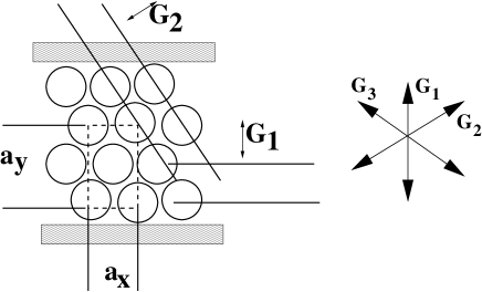
Figure 1: The confined solid is shown along with the centered rectangular (CR) unit cell. For an unstrained triangular lattice $a_{x}=a_{0}$ and $a_{y}=\sqrt{3}a_{0}$. ${\bf G_{1}}$, ${\bf G_{2}}$ and ${\bf G_{3}}$ denote the directions of the three reciprocal lattice vectors (RLV). Note that the third reciprocal lattice direction ${\bf G_{3}}$ is equivalent to ${\bf G_{2}}$, even in the presence of the walls.

The wall- particle interaction potential $V_{\rm wall}(y)=0$ for ${d/2}<y<L_{y}-{d/2}$ and $=\infty$ otherwise. Here, evidently, $L_{y}$ is the width of the channel. The length of the channel is $L_{x}$ with $L_{x}\gg L_{y}$. Periodic boundary conditions are assumed in the $x$ direction(Fig.1).

Before we go on to describe the various phases we observe in this model system, it is instructive to consider how a triangular lattice (the ground state configuration) may be accomodated within a pair of straight hard walls. For the channel to accommodate $n_{l}$ layers of a homogeneous, triangular lattice with lattice parameter $a_{0}$ of hard disks of diameter ${d}$, (Fig.6) it is required that,

$$L_{y}=\frac{\sqrt{3}}{2}(n_{l}-1)a_{0}+{d}~{}.$$ (1)

For a system of constant number of particles and $L_{y}$, $a_{0}$ is a function of packing fraction $\eta$ alone. We define $\chi(\eta,L_{y})=1+2(L_{y}-{d})/\sqrt{3}a_{0}$, so that the above condition reads $\chi={\rm integer}=n_{l}$ (the commensurate configuration) and violation of Eq.(1) implies a rectangular strain away from the reference triangular lattice of $n_{l}$ layers. The lattice parameters of a centered rectangular (CR) unit cell are $a_{x}$ and $a_{y}$ (Fig. 1). In general, for a CR lattice with a given $L_{y}$, $a_{y}=2(L_{y}-{d})/(n_{l}-1)$ and $a_{x}=2/\rho a_{y}$, ignoring vacancies. There are two distinct classes of close packed planes in the CR lattice. Due to the presence of confinement, even for a triangular lattice, the set of planes with reciprocal lattice vector (RLV) ${\bf G_{1}}=\hat{y}\frac{4\pi}{a_{y}}$ perpendicular to the walls are distinct from the equivalent set of planes with the RLV’s ${\bf G_{2}}=\hat{x}\frac{4\pi}{a_{y}}\cos(\frac{\pi}{6})+\hat{y}\frac{4\pi}{a_{y}}\sin(\frac{\pi}{6})$ and ${\bf G_{3}}=\hat{x}\frac{4\pi}{a_{y}}\cos(\frac{\pi}{6})-\hat{y}\frac{4\pi}{a_{y}}\sin(\frac{\pi}{6})$ (Fig.1).

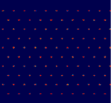
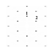
Figure 2: (Colour online) Solid: Left panel shows a picture of $10^{3}$ uncorrelated, superimposed configurations of a high density ($\eta=0.85$) solid phase. The wall to wall separation is commensurate with a ten layered solid at the given density. The colour code is such that red (light) means high local density and blue (dark) means low density. The right panel shows the corresponding structure factor which shows a pattern typical for a two dimensional triangular solid.

Anticipating some of the discussion in section IV, we point out two different but equivalent “pictures” for studying the deformation behavior of confined narrow crystalline strips. In the first picture, the stress is regarded as a function of the “external” strain. Using the initial triangular solid (packing fraction $\eta_{0}$) as reference, the external strain associated with changing $L_{x}$ at a constant $N$ and $L_{y}$ is $\epsilon=(L_{x}-L_{x}^{0})/L_{x}^{0}$. In this case we obtain the stress as an oscillating non-monotonic function of $\epsilon$. On the other hand, internally, the solid is, free to adjust $n_{l}$ to decrease its energy (strain). Therefore, one may, equivalently, calculate strains with respect to a reference, distortion-free, triangular lattice at $\eta$. Using the definition $\varepsilon_{d}=\varepsilon_{xx}-\varepsilon_{yy}=(a_{x}-a_{0})/a_{0}-(a_{y}-\sqrt{3}a_{0})/\sqrt{3}a_{0}=a_{x}/a_{0}-a_{y}/\sqrt{3}a_{0}$ and the expressions for $a_{x}$, $a_{y}$ and $a_{0}=2(L_{y}-d)/\sqrt{3}(\chi-1)$ we obtain,

$$\varepsilon_{d}=\frac{n_{l}-1}{\chi-1}-\frac{\chi-1}{n_{l}-1},$$ (2)

where the number of layers $n_{l}$ is the nearest integer to $\chi$ so that $\varepsilon_{d}$ has a discontinuity at half -integral values of $\chi$. For large $L_{y}$ this discontinuity and $\varepsilon_{d}$ itself vanishes as $1/L_{y}$ for all $\eta$. This “internal” strain $\varepsilon_{d}$ is related non-linearly to $\epsilon$ and may remain small even if $\epsilon$ is large. The stress is always a monotonic function of $\varepsilon_{d}$. Note that a pair of variables $\eta$ and $L_{y}$ (or alternately $\epsilon$ and $\chi$) uniquely fixes the state of the system.

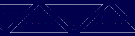
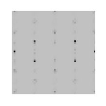
Figure 3: (Colour online) Buckled phase: A small incommensuration is introduced by increasing the wall to wall separation from the value commensurate to a high density ten layered triangular solid at $\eta=0.89$. This reduces the packing fraction to $\eta=0.85$ and produces this phase. The upper panel shows a picture of $10^{3}$ superimposed configurations. The colour code for the local densities is the same as Fig.2. Note that different portions of triangular solid are displaced along $y$- direction to span the extra space introduced between the walls. Lines are drawn to identify this shift in triangular regions. The lower panel shows the corresponding structure factor where the peak in ${\bf G}_{1}$ direction is diminished. Some extra weak peaks corresponding to super-lattice reflections appear at lower values of the wave-number.

We have carried out extensive Monte Carlo (MC) simulations in the constant NAT ensemble using standard Metropolis updates for hard disks (i.e. moves are rejected if they lead to overlaps). The initial condition for our simulations is the perfectly commensurate triangular lattice with a fixed number of layers $n_{l}$ and at a fixed packing fraction $\eta$. After equilibration for typically about $10^{6}$ Monte Carlo steps (MCS), a strain $\epsilon$ is imposed by rescaling $L_{x}$. Since the walls are kept fixed, this strain reduces $\eta$. The sequence of phases and the nature of the transitions among them induced by this strain is discussed below.

III Structures and Phases

In Q1D long wavelength fluctuationsricci2 are expected to destroy all possible order except for those imposed by explicit (as opposed to spontaneous) breaking of symmetry. The confining potential, in the case of a Q1D system in a hard wall channel, explicitly breaks the continuous rotational symmetry down to a ${\cal Z}_{2}$ symmetry (rotations by angle $\pm\pi$). This immediately leads to all $2n$-atic bond orientational orders, like nematic ($n=1$), square ($n=2$), hexatic ($n=3$) etc. which remain nonzero throughout the phase diagram. This situation is therefore similar to a system in a periodic laser potentialfrey-lif-prl ; lif-hd ; mylif . Apart from orientational symmetry, the confining potential explicitly breaks translational symmetry perpendicular to the walls leading to a density modulation in that direction. Any fluctuation which leads to global changes in the direction of layering or in the layer spacing for fixed wall to wall separation is strongly suppressed.

For finite systems (and over finite - but very long - times) of confined Q1D strips one obtains long-lived, metastable ordered phases which are observable even in experimentspieranski-1 . It is these ‘phases’ that we describe in this section. For convenience in nomenclature, we continue to use the terms solid, modulated liquid and smectic to denote these phases, though keeping in mind that the distinctions are largely quantitative and not qualitative. For example, a weak solid-like local hexagonal modulation is present on top of the smectic layering order in what we call the smectic phase. The smectic develops continuously and smoothly from the modulated liquid. We also denote the sharp changes in observables (eg. strength of diffraction peaks) as “phase transitions” though they can never be classified as true phase transitions in the sense of equilibrium thermodynamics. We show, however, that these phase transitions may be described within MFTs (section V) although they might loose meaning when fluctuations are considered in the limit of infinite observation time.

In our description of the phases we make use of the structure factor

$$S_{\bf G}=\left<\frac{1}{N^{2}}\sum_{j,k=1}^{N}\exp(-i{\bf G}.{\bf r}_{jk})\right>,$$

where ${\bf r}_{ij}={\bf r}_{j}-{\bf r}_{i}$ with ${\bf r}_{i}$ the position vector of particle $i$. We shall use particularly the values of $S_{\bf G}$ for the reciprocal lattice vectors ${\bf G}=\pm{\bf G_{1}}(\eta)$ and ${\bf\pm G_{2}}(\eta)$. Notice that ${\bf\pm G_{2}}(\eta)$ and ${\bf\pm G_{3}}(\eta)$ as shown in Fig.1 are equivalent directions. A plot of $S_{\bf G}$ for ${\bf G}=(G_{x},G_{y})$ in the two dimensional plane gives the diffraction pattern observable in scattering experiments. For every phase discussed below, the diffraction pattern always shows at least two peaks corresponding to $\pm{\bf G}_{1}$ since they represent the density modulation imposed by the walls. The relative strengths of these peaks, of course, depend on the structure of the phase concerned.

If the separation between the hard walls is kept commensurate such that $\chi=n_{l}$, an integer, at high density we obtain a perfect two dimensional triangular solid (Fig.2). The solid shows a diffraction pattern which is typical for a two dimensional triangular crystal. We show later that appearances can be deceptive, however. This triangular “solid” is shown to have zero shear modulus which would mean that it can flow without resistance along the length of the channel like a liquid. Stretching the solid strip lengthwise, on the other hand, costs energy and is resisted. The strength of the diffraction peaks decreases rapidly with the order of the diffraction. In strictly two dimensions this is governed by a non-universal exponent dependent on the elastic constants kthny1 . In Q1D this decay should be faster. However, larger system sizes and averaging over a large number of configurations would be required to observe this decay, since constraints placed by the hard walls make the system slow to equilibrate at high densities. For a general value of $\chi$ the lattice is strained which shows up in the relative intensities of the peaks in the diffraction pattern corresponding to ${\bf G}_{2}$ and ${\bf G}_{3}$.

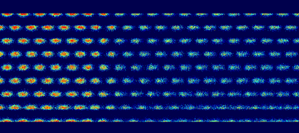
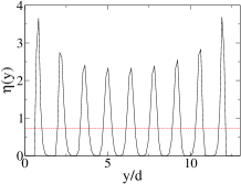
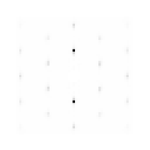
Figure 4: (Colour online) Smectic: A confined triangular solid at $\eta=0.85$ is strained in $x$-direction to a packing fraction $\eta=0.73$. The upper panel shows a picture of $10^{3}$ superimposed configurations. The colour code for local density is same as Fig.2. The lower left panel shows the density modulation in $y$- direction. The lower right panel shows the corresponding structure factor where the only remaining strong peaks are in ${\bf G}_{1}$ direction identifying a smectic order (solid-like in $y$-direction and liquid-like in other directions). This smectic phase, however, possesses hexagonal modulations producing weak triangular order leading to faint secondary spots in the structure factor.

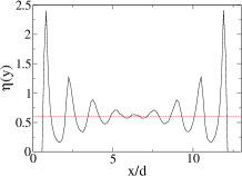
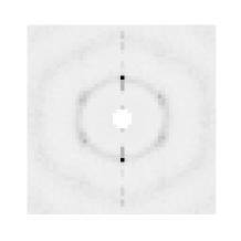
Figure 5: (Colour online) Modulated liquid: A confined triangular solid at $\eta=0.85$ is strained in $x$-directon reducing the density to $\eta=0.6$. The upper panel shows a picture of $10^{3}$ superimposed configurations. The colour code of local densities is the same as Fig.2. The lower left panel shows the density modulation in $y$- direction which is like the smectic phase but the modulation dies out at the center. The structure factor in the lower right panel shows a ring like pattern which is a typical signature of liquid. Superimposed on this are strong smectic-like peaks in ${\bf G}_{1}$ direction.

A little extra space introduced between the walls starting from a high density solid phase gives rise to buckling instability in $y$- direction and the system breaks into several triangular solid regions along the $x$- direction (Fig.3). Each of these regions slide along close packed planes (corresponding to the reciprocal directions ${\bf G}_{2}$ or ${\bf G}_{3}$) with respect to one another. This produces a buckling wave with displacement in $y$- direction travelling along the length of the solid. In conformity with the quasi two dimensional analog buckled-1 ; buckled-2 ; buckled-3 we call this the buckled solid and it interpolates continuously from $\chi=n_{l}$ to $n_{l}\pm 1$ layers. This phase can also occur due to the introduction of a compressional strain in $x$-direction keeping $L_{y}$ fixed. The diffraction pattern shows a considerable weakening of the spots corresponding to planes parallel to the walls $S_{\bf G_{1}}$ together with generation of extra spots at smaller wave-number corresponding to the buckled super-lattice. The diffraction pattern is therefore almost complementary to that of the smectic phase to be discussed below. We do not observe the buckled solid at low densities close to the freezing transition. Large fluctuations at such densities lead to creation of bands of the smectic phase within a solid eventually causing the solid to melt.

At low enough densities or high enough in-commensuration ($\chi$ half integral) the elongated density profiles in the lattice planes parallel to the walls can overlap to give rise to what we denote as the smectic phase (Fig.4) in which local density peaks are smeared out in $x$- direction but are clearly separated in $y$-direction giving rise to a layered structure. The diffraction pattern shows only two strong spots ($S_{\bf G_{1}}$) which is typical corresponding to the symmetry of a smectic phase. We use this fact as the defining principle for this phase. Note that unlike usual smectics there is no orientational ordering of director vectors of the individual particles since hard disks are isotropic.

At further lower densities the relative displacement fluctuations between neighbors diverges and the diffraction pattern shows a ring- like feature typical of a liquid which appears together with the smectic like peaks in the direction perpendicular to the walls. We monitor this using the relative Lindemann parameterpcmp , given by,

$$l=\langle({u^{x}}_{i}-{u^{x}}_{j})^{2}\rangle/a_{x}^{2}+\langle({u^{y}}_{i}-{u^{y}}_{j})^{2}\rangle/a_{y}^{2}$$ (3)

where the angular brackets denote averages over configurations, $i$ and $j$ are nearest neighbors and ${u^{\alpha}}_{i}$ is the $\alpha$-th component of the displacement of particle $i$ from it’s mean position. This phase is a modulated liquid (Fig.5). The density modulation decays away from the walls and for large $L_{y}$, the density profile in the middle of the channel becomes uniform. A clear structural difference between smectic and modulated liquid is the presence of the ring pattern in the structure factor of the latter, a characteristic of liquid phase (compare Fig.4 and 5). We must emphasize here again that the distinction between a modulated liquid and a smectic is mainly a question of degree of the layering modulation. The two structures merge continuously into one another as the density is increased. Also when the modulated liquid co-exists with the solid, the layering in the former is particularly strong due to proximity effects.

IV Mechanical Properties and Failure

In this section we present the results for the mechanical behavior and failure of the Q1D confined solid under tension. We know that fracture in bulk solids occurs by the nucleation and growth of cracksgriffith ; marder-1 ; marder-2 ; langer . The interaction of dislocations or zones of plastic deformationlanger ; loefsted with the growing crack tip determines the failure mechanism viz. either ductile or brittle fracture. Studies of the fracture of single-walled carbon nanotubesSWCNT-1 ; SWCNT-2 show failure driven by bond-breaking which produces nano cracks which run along the tube circumference leading to brittle fracture. Thin nano-wires of Ni are knownnano-wire-1 ; nano-wire-2 to show ductile failure with extensive plastic flow and amorphization. We show that the Q1D confined solid behaves anomalously, quite unlike any of the mechanisms mentioned above. It shows reversible plastic deformation and failure in the constant extension ensemble. The failure occurs by the nucleation and growth of smectic regions which occur as distinct bands spanning the width of the solid strip.

Figure 6: Results of NAT ensemble MC simulations of $N=n_{x}\times n_{y}=65\times 10$ hard disks confined between two parallel hard walls separated by a distance $L_{y}=9\,{d}$. For each $\eta$, the system was allowed to run for $10^{6}$ MCS and data averaged over a further $10^{6}$ MCS. At $\eta=0.85$ we have a strain free triangular lattice. Plots show the structure factors $S_{\bf G_{i}},i=1(+),2(\diamond)$ for RLVs ${\bf G_{i}}(\eta)$, averaged over symmetry related directions, as a function of $\eta$. Also plotted in the same graph is the Lindemann parameter $l(\Box)$. The lines in the figure are a guide to the eye.

We study the effects of strain on the hard disk triangular solid for a $L_{y}$ large enough to accommodate only a small number of layers $n_{l}\sim 9-25$. The Lindemann parameter $l$ diverges at the melting transition Zahn . We also compute the quantities $S_{{\bf G=G}_{1}}$ and $S_{{\bf G=G}_{2}}$.

In Fig.6 we show how $S_{\bf G_{2}},~{}S_{\bf G_{1}}$ and $l$ vary as a function of externally imposed elongational strain that reduces $\eta$. Throughout, $S_{\bf G_{2}}<S_{\bf G_{1}}\neq 0$. This is a consequence of the hard wall constrainthartmut which induces an oblate anisotropy in the local density peaks of the solid off from commensuration (nonintegral $\chi$). As $\eta$ is decreased both $S_{\bf G_{1}}$ and $S_{\bf G_{2}}$ show a sharp drop at $\eta=\eta_{c_{1}}$ where $\chi=\chi^{\ast}\approx n_{l}-1/2$ [Fig. 7 (inset) ]. For $\eta<\eta_{c_{1}}$ we get $S_{\bf G_{2}}=0$ with $S_{\bf G_{1}}\not=0$ signifying a transition from crystalline to smectic like order. The Lindemann parameter $l$ remains zero and diverges only below $\eta=\eta_{c_{3}}(\approx\eta_{m})$ indicating a finite-size- broadened “melting” of the smectic to a modulated liquid phase.

To understand the mechanical response of the confined strips, we compute the deviatoric stress built up in the system as a function of applied strain. The stress tensor of a bulk system interacting via two body central potential has two parts: (i) A kinetic part $\sigma^{K}_{\lambda\nu}$ leading to an isotropic pressure and (ii) A virial term due to inter-particle interaction $\sigma^{int}_{\lambda\nu}$. The free-particle-like kinetic component of the stress $\beta\sigma^{K}_{\lambda\nu}=-\rho\delta_{\lambda\nu}$ and the component due to inter-particle interaction $\sigma^{int}_{\lambda\nu}=-\langle\sum_{<ij>}r_{ij}^{\lambda}f_{ij}^{\nu}\rangle/S$ with $f^{\nu}_{ij}$ the $\nu$-th component of inter-particle force, $S=L_{x}L_{y}$ area of the strip. The expression for the stress tensor for the bulk system of hard disks translates toelast

$$\beta\sigma_{\lambda\nu}d^{2}=-\frac{d^{2}}{S}\left(\sum_{<ij>}\left<\delta(r_{ij}-d)~{}\frac{r^{\lambda}_{ij}r^{\nu}_{ij}}{r_{ij}}\right>+N\delta_{\lambda\nu}\right).$$ (4)

The presence of walls gives rise to a potential which varies only in the $y$-direction perpendicular to the walls. Therefore, strains $\epsilon_{xx}$ and $\epsilon_{xy}$ do not lead to any change in the wall induced potential. As a consequence the conjugate stresses for the confined system $\sigma^{C}_{xx}=\sigma_{xx}$ and $\sigma^{C}_{xy}=\sigma_{xy}$. However, a strain $\epsilon_{yy}$ does lead to a change in potential due to the walls and therefore a new term in the expression for conjugate stress appearsmylif-large , $\sigma_{yy}^{C}=\sigma_{yy}+\sigma^{w}$ with $\sigma^{w}=-\langle\sum_{<iw>}f^{w}_{i}y_{iw}\rangle/S$ where $w$ denotes the two confining walls. This expression can be easily understood by regarding the two walls as two additional particles of infinite massvarnik . Thus, to obtain the component of the total stress normal to the walls from MC simulations we use

$$\beta\sigma_{yy}^{C}d^{2} = \beta\sigma_{yy}d^{2}-\frac{d^{2}}{S}\left[\left\langle\sum_{i}y_{i}\delta(y_{i}-d/2)\right\rangle\right.$$ (5)

$$+ \left.\left\langle\sum_{i}(L_{y}-y_{i})\delta(L_{y}-y_{i}-d/2)\right\rangle\right].$$

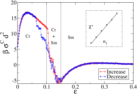
Figure 7: (Colour online) A plot of the deviatoric stress $\sigma^{C}$ versus external strain $\epsilon$ obtained from our MC simulations of $65\times 10$ hard disks initially at $\eta=0.85$ and $L_{y}=9d$. Data is obtained by holding at each strain value for $2\times 10^{4}$ MCS and averaging over a further $3\times 10^{4}$ MCS. The entire cycle of increasing $\epsilon(\circ)$ and decreasing to zero $(\Box)$ using typical parameters appropriate for an atomic system, corresponds to a real frequency of $\omega\approx 25{\rm K\,Hz}$. Results do not essentially change for $\omega=1{\rm K\,Hz}\,-1{\rm M\,Hz}$. The line is a guide to the eye. The vertical lines mark the limit of stability of the crystal (Cr), the two phase region (Cr+Sm) and the onset of the smectic phase (Sm). Inset shows the variation of the critical $\chi^{\ast}$ with $n_{l}$, points: simulation data; line: $\chi^{\ast}=n_{l}-1/2$.

The deviatoric stress, $\sigma^{C}=\sigma^{C}_{xx}-\sigma^{C}_{yy}$, versus strain, $\epsilon=\epsilon_{xx}-\epsilon_{yy}$ ($\epsilon_{yy}=0$) curve for confined hard disks is shown in Fig. 7. For $\eta=\eta_{0}$ ($\epsilon=0$) the stress due to the inter-particle interaction is purely hydrostatic with $\sigma_{xx}=\sigma_{yy}$ as expected; however, due to the excess pressure from the walls the solid is actually always under compression along the $y$ direction, thus $\sigma_{xx}^{C}>\sigma_{yy}^{C}$. At this point the system is perfectly commensurate with channel width and the local density profiles are circularly symmetric.

Initially, the stress increases linearly, flattening out at the onset of plastic behavior at $\eta\stackrel{{\scriptstyle<}}{{\sim}}\eta_{c_{1}}$. At $\eta_{c_{1}}$, with the nucleation of smectic bands, $\,\,\sigma^{C}$ decreases and eventually becomes negative. At $\eta_{c_{2}}$ the smectic phase spans the entire system and $\sigma^{C}$ is minimum. On further decrease in $\eta$ towards $\eta_{c_{3}}$, $\sigma^{C}$ approaches $0$ from below (Fig. 7) thus forming a loop. Eventually it shows a small overshoot, which ultimately goes to zero, from above, as the smectic smoothly goes over to a more symmetric liquid like phase – thus recovering the Pascal’s law at low enough densities. If the strain is reversed by increasing $\eta$ back to $\eta_{0}$ the entire stress-strain curve is traced back with no remnant stress at $\eta=\eta_{0}$ showing that the plastic region is reversible. For the system shown in Fig.1 we obtained $\eta_{c_{1}}\approx 0.77$, $\eta_{c_{2}}\approx 0.74$ and $\eta_{c_{3}}\approx 0.7$. As $L_{y}$ is increased, $\eta_{c_{1}}$ merges with $\eta_{c_{3}}$ for $n_{l}\stackrel{{\scriptstyle>}}{{\sim}}25$. If instead, $L_{x}$ and $L_{y}$ are both rescaled to keep $\chi=n_{l}$ fixed or PBCs are imposed in both $x$ and $y$ directions, the transitions in the various quantities occur approximately simultaneously as expected in the bulk system. Varying $n_{x}$ in the range $50-5000$ produces no qualitative change in most of the results.

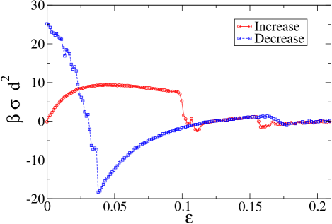
Figure 8: (Colour online) A plot of the deviatoric stress $\sigma$ versus external strain $\epsilon$ obtained from our MC simulations of $65\times 10$ hard disks, in presence of PBCs in both the directions, initially a triangular lattice at $\eta=0.85$. Data is obtained by holding at each strain value for $2\times 10^{4}$ MCS and averaging over a further $3\times 10^{4}$ MCS. The entire cycle of increasing $\epsilon(\circ)$ and decreasing to zero $(\Box)$ using typical parameters appropriate for an atomic system, corresponds to a real frequency of $\omega\approx 100{\rm K\,Hz}$. The line through the points is guide to the eye.

Reversible plasticity in the confined narrow strip is in stark contrast with the mechanical response of a similar strip in the absence of confinement. In order to show this, we study a similar narrow strip of $65\times 10$ hard disks but now we use PBCs in both the directions. At packing fraction $\eta=0.85$ the initial geometry ($L_{x}^{0}=65a_{x}$, $L_{y}=10a_{y}$ with $a_{y}=\sqrt{3}a_{x}/2$) contains a perfect triangular lattice. We impose strain in a fashion similar to that described in Fig.7. The resulting stress-strain curve is shown in Fig.8. With increase in strain $\epsilon$ the system first shows a linear (Hookean) response in the deviatoric stress $\sigma=\sigma_{xx}-\sigma_{yy}$, flattening out at the onset of plastic deformation below $\epsilon\sim 0.1$. Near $\epsilon=0.1$ with a solid-liquid transition (solid order parameter drops to zero with divergence of Lindeman parameter at the same strain value) the deviatoric stress $\sigma$ decreases sharply to zero in the liquid phase obeying the Pascal’s law. Unlike in the confined strip, with further increase in strain $\sigma$ does not become negative and fluctuates around zero in absence of wall induced density modulations. With decrease in strain, starting from the liquid phase, the stress $\sigma$ does not trace back its path. Instead first a large negative stress is built up in the system as we decrease strain up to $\epsilon\sim 0.04$. With further decrease in $\epsilon$, the stress $\sigma$ starts to increase and at $\epsilon=0$ the system is under a huge residual stress $\beta\sigma d^{2}=25$. The configuration of the strip at this point shows a solid with lattice planes rotated with respect to the initial stress-free lattice. This solid contains defects. Note that in the presence of hard confining walls, global rotation of the lattice planes cost large amounts of energy and would be completely suppressed. The generation of defects is also difficult in a confined system unless they have certain special characteristics which we describe later.

For a confined Q1D strip in the density range $\eta_{c_{2}}<\eta<\eta_{c_{1}}$ we observe that the smectic order appears within narrow bands (Fig. 9). Inside these bands the number of layers is less by one and the system in this range of $\eta$ is in a mixed phase. A plot (Fig.9 (a) and (b)) of $\chi(x,t)$, where we treat $\chi$ as a space and time (MCS) dependent “order parameter” (configuration averaged number of layers over a window in $x$ and $t$), shows bands in which $\chi$ is less by one compared to the crystalline regions. After nucleation, narrow bands coalesce to form wider bands over very large time scales. The total size of such bands grow as $\eta$ is decreased. Calculated diffraction patterns (Fig. 9 (c) and (d)) show that, locally, within a smectic band $S_{\bf G_{1}}\gg S_{\bf G_{2}}$ in contrast to the solid region where $S_{\bf G_{1}}\approx S_{\bf G_{2}}\neq 0$.

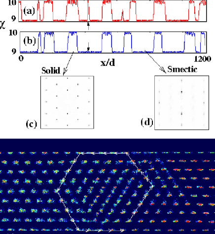
Figure 9: (Colour online) Plot of $\chi(x,t)$ as a function of the channel length $x/d$ at $\eta=0.76$ after time $t=$ (a)$5\times 10^{5}$ and (b)$2\times 10^{6}$ MCS for $N=10^{3}\times 10$ with $L_{y}=9d$. Note that $\chi=10$ in the solid and $\chi=9$ in the smectic regions. Arrows show the coalescence of two smectic bands as a function of time. Calculated diffraction patterns for the (c) $10$-layered solid and (d) $9$-layered smectic regions. (e) Close up view of a crystal-smectic interface from $10^{3}$ superimposed configurations at $\eta=0.77$. The colour code of the local density is the same as Fig.2. Note the misfit dislocation in the inter-facial region. A Burger’s circuit is shown to identify the Burger’s vector corresponding to this dislocation as $\vec{b}=\hat{y}a_{y}/2+\hat{x}a_{x}/2$.

Noting that $\chi=\chi^{\ast}=n_{l}-1/2$ when the solid fails (Fig. 7 inset), it follows from Eq. 2, the critical strain $\varepsilon_{d}^{\ast}=(4n_{l}-5)/(2n_{l}-3)(2n_{l}-2)\sim 1/n_{l}$. This is supported by our simulation data over the range $9<n_{l}<14$. This shows that thinner strips (smaller $n_{l}$) are more resistant to failure. At these strains the solid generates bands consisting of regions with one less particle layer. Within these bands adjacent local density peaks of the particles overlap in the $x$ direction producing a smectic. Within a simple density functional argumentrama it can be shown that the spread of local density profile along $x$-axis $\alpha_{x}\sim 1/\sqrt{S_{\bf G_{2}}}$ and that along $y$-direction is $\alpha_{y}\sim 1/\sqrt{2S_{\bf G_{1}}+S_{\bf G_{2}}}$ myijp . In the limit $S_{\bf G_{2}}\to 0$ (melting of solid) $\alpha_{x}$ diverges though $\alpha_{y}$ remains finite as $S_{\bf G_{1}}$ remains positive definite. Thus the resulting structure has a smectic symmetry.

A superposition of many particle positions near a solid-smectic interface [see Fig. 9(e)] shows that: $(1)$ The width of the interface is large, spanning about $10-15$ particle spacings. $(2)$ The interface between $n_{l}$ layered crystal and $n_{l}-1$ layered smectic contains a dislocation with Burger’s vector in the $y$- direction which makes up for the difference in the number of layers. Each band of width $s$ is therefore held in place by a dislocation-anti-dislocation pair (Fig. 9). In analogy with classical nucleation theorypcmp ; cnt , the free energy $F_{b}$ of a single band can be written as

$$F_{b}=-\delta Fs+E_{c}+\frac{1}{8\pi}b^{2}K^{\Delta}\log\frac{s}{a_{0}}$$ (6)

where $K^{\Delta}$ is an elastic constant, ${\vec{b}}=\hat{y}a_{y}/2+\hat{x}a_{x}/2$ is the Burger’s vector, $\delta F$ the free energy difference between the crystal and the smectic per unit length and $E_{c}$ the core energy for a dislocation pair. Bands form when dislocation pairs separated by $s>\frac{1}{8\pi}b^{2}K^{\Delta}/\delta F$ arise due to random fluctuations. To produce a dislocation pair a large energy barrier of core energy $E_{c}$ has to be overcome. Though even for very small strains $\varepsilon_{d}$ the elastic free energy becomes unstable the random fluctuations can not overcome this large energy barrier within finite time scales thereby suppressing the production of $n_{l}-1$ layered smectic bands up to the point of $\varepsilon_{d}^{\ast}$. In principle, if one could wait for truly infinite times the fluctuations can produce such dislocation pairs for any non-zero $\varepsilon_{d}$ though the probability for such productions $\exp(-\beta E_{c})$ [$\beta=1/k_{B}T$, inverse temperature] are indeed very low. Using a procedure similar to that used in Ref.sura-hdmelt ; mylif ; mylif-large , we have monitored the dislocation probability as a function of $\eta$ (Fig.10). For confined hard disks, there are essentially three kinds of dislocations with Burger’s vectors parallel to the three possible bonds in a triangular solid. Only dislocations with Burger’s vectors having components perpendicular to the walls, cause a change in $n_{l}$ and are therefore relevant. The dislocation formation probability is obtained by performing a simulation where the local connectivity of bonds in the solid is not allowed to change while an audit is performed of the number of moves which tend to do so. Since each possible distortion of the unit cell (see Fig.10 - inset) can be obtained by two specific sets of dislocations, the dislocation probabilities may be easily obtained from the measured probability of bond breaking moves.

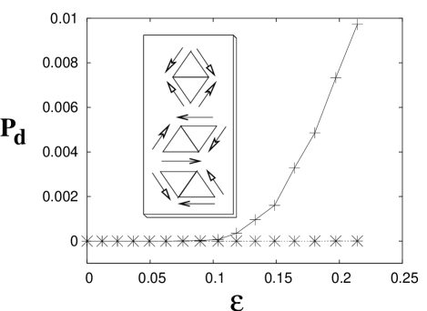
Figure 10: Dislocation probabilities of a $65\times 10$ system are plotted as a function of strain starting from a triangular solid at $\eta=0.85$ and $L_{y}=9d$. The corresponding bond-breaking moves are depicted in the inset panel. Arrows show the directions of the bond-breaking moves. $+$ show dislocation probabilities for those Burger’s vectors which have components perpendicular to the walls (topmost figure in the inset). On the other hand probabilities corresponding to the other two types of moves (denoted by $\ast$) remain zero.

Not surprisingly, the probability of obtaining dislocation pairs with the relevant Burger’s vector increases dramatically as $\eta\to\eta_{c_{1}}$ (Fig.10) and artificially removing configurations with such dislocations suppresses the transition completely. Band coalescence occurs by diffusion aided dislocation “climb” which at high density implies slow kinetics. The amount of imposed strain fixes the total amount of solid and smectic regions within the strip. The coarsening of the smectic bands within the solid background in presence of this conservation, leads to an even slower dynamics than non-conserving diffusion. Therefore the size of smectic band $L(t)$ scales as $L\sim t^{1/3}$bray . Throughout the two-phase region, the crystal is in compression and the smectic in tension along the $y$ direction so that $\sigma$ is completely determined by the amount of the co-existing phases. Also the walls ensure that orientation relationships between the two phases are preserved throughout. As the amount of solid or smectic in the system is entirely governed by the strain value $\epsilon$ the amount of stress $\sigma^{C}$ is completely determined by the value of strain at all times regardless of deformation history. This explains the reversibleonions plastic deformation in Fig. 7.

V The Mean Field Phase Diagram

In this section we obtain the phase diagram from Monte Carlo simulations of $65\times n_{l}$ hard disks, $n_{l}$ being the number of layers contained within the channel. We compare this with a MFT calculation. At a given $L_{y}$ we start with the largest number of possible layers of particles and squeeze $L_{x}$ up to the limit of overlap. Then we run the system over $5\times 10^{4}$ MCS, collect data over further $5\times 10^{4}$ MCS and increase $L_{x}$ in steps such that it reduces the density by $\delta\eta=0.001$ in each step. At a given $L_{y}$ and $n_{l}$ the value of $L_{x}$ that supports a perfect triangular lattice has a density

$$\eta_{\triangle}=\frac{\sqrt{3}\pi}{8}\frac{n_{l}(n_{l}-1)}{L_{y}(L_{y}-1)}.$$ (7)

In this channel geometry, at phase coexistence, the stress component $\sigma_{xx}$ of the coexisting phases becomes equal. The other component $\sigma_{yy}$ is always balanced by the pressure from the confining walls. Thus we focus on the quantity $p_{x}=-\sigma_{xx}$ as $L_{x}$ is varied:

$$p_{x}=-\frac{1}{L_{y}}\frac{\partial F}{\partial L_{x}}=\rho^{2}\frac{\partial f_{N}}{\partial\rho},~{}\frac{\partial f_{N}}{\partial\rho}=\frac{p_{x}}{\rho^{2}}.$$ (8)

The free energy per unit volume $f_{V}=(N/V)(F/N)=\rho f_{N}$. One can obtain the free energy at any given density $\rho$ by integrating the above differential equation starting from a known free energy at some density $\rho_{0}$,

$$f_{V}(\rho)=\rho f_{N}^{0}(\rho_{0})+\rho\int_{\rho_{0}}^{\rho}\frac{p_{x}}{\rho^{2}}d\rho~{}.$$ (9)

We discuss below how $f_{N}^{0}(\rho_{0})$ for solid and modulated liquid phases are obtained. The free energy of the solid phase may be obtained within a simple analytical treatment viz. fixed neighbor free volume theory (FNFVT), which we outline below. More detailed treatment is available in Ref.my-htcond . The free volume $v_{f}(\eta,\chi)$ may be obtained using straight forward, though rather tedious, geometrical considerations and the free energy $f_{N}^{0}(\eta,\chi)=-\rho\ln v_{f}(\eta,\chi)$. The free volume available to a particle is computed by considering a single disk moving in a fixed cage formed by its nearest neighbors which are assumed to be held in their average positions. The free volume available to this central particle (in units of $d^{2}$) is given entirely by the lattice separations $b=a_{0}(1+\epsilon_{xx})$ and $h=\sqrt{3}a_{0}(1+\epsilon_{yy})/2$ where $a_{0}$ is lattice parameter of a triangular lattice at any given packing fraction $\eta$ and $\epsilon_{xx}=(n_{l}-1)/(\chi-1)$, $\epsilon_{yy}=1/\epsilon_{xx}$. As stated in Sec.II, $\chi$ is obtained from channel width $L_{y}$ and packing fraction $\eta$. $v_{f}$ is the area available to the central test particle. Note that the effect of the confining geometry is incorporated in the lattice separations $b$, $h$. The FNFVT free energy has minima at all $\chi=n_{l}$. For half integral values of $\chi$ the homogeneous crystal is locally unstable. Although FNFVT fails also at these points, this is irrelevant as the system goes through a phase transition before such strains are realized. In the high density triangular solid phase, we know $f_{N}^{0}(\rho_{0}=\rho_{\triangle})$, exactly, from the fixed neighbor free volume theory (FNFVT). It is interesting to note that, apart from at $\rho_{\triangle}$, this FNFVT can estimate the solid free energy quite accurately at small strains $\epsilon_{xx}<4\%$ around $\rho_{\triangle}$. To obtain the solid branch of free energy $f^{S}_{V}(\rho)$ from simulations, we integrate the $p_{x}-\rho$ curve starting from the FNFVT estimate at $\rho=\rho_{0}\equiv\rho_{\triangle}$.

For the confined fluid phase we use a phenomenological free energy santos of hard disk fluid added with a simple surface tension term due to the scaled particle theory spt . We outline this in the following. For the bulk (unconfined) liquid phase one can obtain $f_{N}^{0}(\rho=\rho_{l})$ up to a fairly large volume fraction $\eta_{l}\sim 0.81$ where the liquid reaches its metastable limit in bulk, using the phenomenological expressionsantos ,

$$\beta f_{N}^{0}(\rho_{l}) = \frac{(2\eta_{c}-1)\ln(1-\frac{2\eta_{c}-1}{\eta_{c}}\eta_{l})-\ln(1-\frac{\eta_{l}}{\eta_{c}})}{2(1-\eta_{c})}$$ (10)

$$+ \ln\rho_{l}-1$$

where $\eta_{c}$ is the close packed volume and depends on $L_{y}$. We have checked from the simulations that this equation of state shows good agreement with the simulated $p_{x}-\eta$ diagram in a confined channel up to a density of $\eta=0.65$. Above this density, $p_{x}$ falls below and $p_{y}$ goes above this equation of state estimate. Integrating $p_{x}$ from $\eta_{0}=\eta_{l}\equiv 0.6$ using the above mentioned form of $f_{N}^{0}(\rho_{l})$ we find the bulk part of the liquid branch of free energy $f^{L}_{V}(\rho)$. In order to incorporate the effect of confinement approximately, we add a scaled particle theory (SPT) spt surface energy contribution to the bulk free energy. Within SPT, the interfacial tension (interfacial energy per unit length) of a hard disk fluid in contact with a hard wall can be calculated as $\gamma=\bar{\gamma}+p_{spt}d/2$ sptlowen where $\bar{\gamma}=(\rho d/2\beta)[1/(1-\eta)-1/(1-\eta)^{2}]$ and the SPT equation of state is $\beta p_{spt}/\rho=1/(1-\eta^{2})$ spt . Thus the SPT surface energy per unit volume $S_{T}=\gamma/L_{y}=\rho d/2\beta(1-\eta)L_{y}$ is added with the bulk contribution $f^{L}_{V}(\rho)$ to account for the confinement.

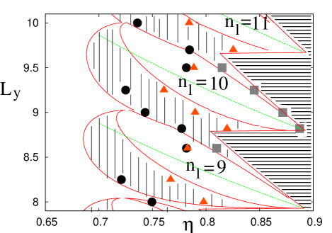
Figure 11: (Colour online) Phase diagram. The continuous lines denote the phase boundaries obtained from mean field theory. The white, vertically shaded and horizontally shaded regions indicate single phase, two-phase coexistence and forbidden regions, respectively. The single phase regions of low densities are liquid and high densities are solid phases. On the green (dashed) lines $n_{l}=9,10,11$ the system is commensurate with the channel width such that exactly integral number of layers are contained. Points denoted by filled $\circ$, filled $\triangle$, and filled $\Box$ are obtained from simulations. Regions with densities less than the filled $\circ$ are modulated liquid and above filled $\triangle$ are solid. In the intervening region, we have a solid-smectic coexistence. The filled $\Box$ mark the onset of buckling instability. Smectic order increases smoothly and continuously as density increases. The liquid within the coexistence region is highly modulated.

At thermodynamic equilibrium, the chemical potential $\mu=-(\partial f_{V}/\partial\rho)_{V,T}$ and pressure for the coexisting phases must be same. Thus from a plot of free energy vs. density obtaining common tangent to solid and liquid branches of free energies means finding coexisting densities of solid and liquid having the same chemical potential. Once the two branches of free energy are obtained in the above mentioned way, we fit each branch using polynomials up to quadratic order in density. The common tangent must share the same slope and intercept. These two conditions uniquely determine the coexisting densities. The onset of buckling instability can be found from the slope of the $p_{x}-\eta$ curve at high densities – a negative slope being the signature of the transition. The estimates of the coexisting densities and onset of the buckling instabilities in our simulations are thus obtained and shown using filled symbols in the phase diagram (Fig.11).

To obtain the phase diagram from MFT (lines in Fig.11) we use the above mentioned phenomenological free energy of hard disk fluidsantos together with the SPT surface tension term. For the solid we use the FNFVT free energy for all densities. We take care to minimize the free energy of the solid with respect to choices of $n_{l}$ first. Then we find out the minimum of the solid and liquid free energies at all densities. The coexisting densities are obtained from common tangent constructions for this minimum free energy. Our MFT phase diagram so obtained is shown along with the simulation results in the $\eta-L_{y}$ plane (Fig.11).

In Fig.11 points are obtained from simulations and the continuous curves from theory. The regions with densities lower than the points denoted by filled circles are single phase modulated liquid. Whereas the regions with densities larger than the points denoted by filled triangles indicate the single phase solid. The modulations in the liquid increase with increasing density and at high enough $\rho$ the structure factor shows only two peaks typical of the smectic phase. This transition is a smooth crossover. All the regions in between the filled circles and filled triangles correspond to solid-smectic coexistence. The filled squares denote the onset of buckling at high densities. The high density regions shaded by horizontal lines are physically inaccessible due to the hard disk overlap. The MFT prediction for the solid-liquid coexistence is shown by the regions between the continuous (red) lines (shaded vertically). The unshaded white regions bounded by red lines and labeled by the number of layers denote the solid phase. All other unshaded regions denote liquid phase. For a constant channel width, a discontinuous transition from liquid to solid via phase coexistence occurs with increasing density. However, the MFT predicts that the solid remelts at further higher densities. Notice that the simulated points for the onset of buckling lie very close to this remelting curve. Since the MFT, as an input, has only two possibilities of solid and fluid phases, the high density remelting line as obtained from the MFT may be interpreted as the onset of instability (buckling) in the high density solid. The MFT prediction of the solid-fluid coexistence region shows qualitative agreement with simulation results for solid-smectic coexistence. The area of phase digram corresponding to the solid phase as obtained from simulation is smaller than that is predicted by the MFT calculation. This may be due to the inability of MFT to capture the effect of fluctuations. From the simulated phase diagram it is clear that if one fixes the density and channel width in a solid phase and then increases the channel width keeping the density fixed, one finds a series of phase transitions from a solid to a smectic to another solid having a larger number of layers. These re-entrant transitions are due to the oscillatory commensurability ratio $\chi$ that one encounters on changing the channel width. This is purely a finite size effect due to the confinement. It is important to note that for a bulk hard disk system, solid phase is stable at $\eta>0.719$, whereas, even for a commensurate confined strip of hard disks, the solid phase is stable only above a density $\eta=0.75$. With increase in incommensuration the density of the onset of solid phase increases further. This means that confinement of the Q1D strip by planar walls has an overall destabilizing effect on the solid phase.

The phase diagram calculated in this section is a MFT phase diagram where the effects of long wavelength (and long time scale) fluctuations are ignored. For long enough Q1D strips fluctuations in the displacement variable should increase linearly destroying all possible spontaneous order and leading to a single disordered fluid phase which is layered in response to the externally imposed hard wall potential. However, even in that limit the layering transitions from lower to higher number of layers as a function of increasing channel width, survivesdegennes .

Our simple theory therefore predicts a discontinuous solid-fluid transition via a coexistence region with change in density or channel width. However, details like the density modulation, effects of asymmetry in density profile, vanishing displacement modes at the walls and most importantly nucleation and dynamics of misfit dislocations crucial to generate the smectic band mediated failure observed in simulations are beyond the scope of this theory. Also, the effect of kinetic constraints which stabilize the solid phase well inside the two phase coexistence region is not captured in this approach. We believe, nevertheless, that this equilibrium calculation may be used as a basis for computations of reaction rates for addressing dynamical questions in the future.

Before we end this section, it is useful to compare our results with similar calculations in higher dimensions viz hard spheres confined within hard parallel plates forming a quasi two dimensional filmbuckled-1 ; fortini ; buckled-3 . Commensuration effects produce non-monotonic convergence of the phase boundaries to that of the bulk system. The appearence of novel phases e.g. the buckled solid not observed in the bulk is also a feature showed by all these systems; on the other hand these quasi two dimensional systems show two kinds of solids – triangular and square – and no ‘smectic like’ phase. The effect of fluctuations also should be much less in higher dimensions and one expects the observed phases to have less anomalous properties.

VI Discussion and Conclusion

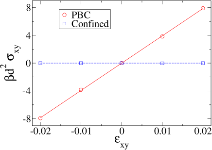
Figure 12: (Colour online) Shear stress vs. shear strain at $\eta=0.85$. A system of $40\times 10$ hard disks simulated with periodic boundary conditions and $L_{y}$ commensurate with ten layered triangular solid gives a shear modulus $\mu=398\pm 4$. On the other hand when the same system of $40\times 10$ hard disks is confined within a commensurate channel, that fits $10$-layers of lattice planes, the shear modulus drops drastically to $\mu=0$.

One of the key definitions of a solid states that a solid, as opposed to a liquid, is a substance which can retain its shape due to its nonzero shear modulus. Going by this definition, a Q1D solid strip even of finite length confined within planar, structureless walls is not a solid despite its rather striking triangular crystalline order. Indeed, the shear modulus of the confined solid at $\eta=0.85$ is zero, though the corresponding system with PBC show finite nonzero shear modulus (See Fig.12). This is a curious result and is generally true for all values of $4<n_{l}<25$ and $\eta$ investigated by us. Confinement induces strong layering which effectively decouples the solid layers close to the walls allowing them to slide past each other rather like reentrant laser induced meltingfrey-lif-prl ; lif-hd ; mylif . This immediately shows that the only thermodynamically stable phase in confined Q1D channel is a modulated liquid, the density modulation coming from an explicit breaking of the translational symmetry by the confinement.

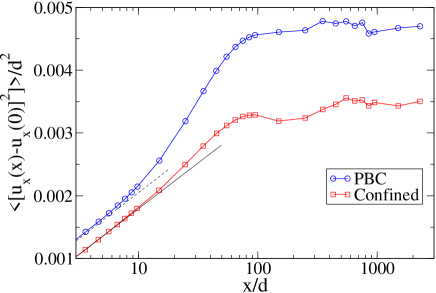
Figure 13: (Colour online) Flucuation $<({u^{x}}(x)-{u^{x}}(0))^{2}>/d^{2}$ on a lattice plane (line) for $5000\times 10$ commensurate triangular solid ($\eta=0.85$) with PBC in both directions is compared with that in presence of hard channel confinement. Averages are done over $100$ configurations. $\circ$ denotes the data obtained in presence of PBC in both directions and $\Box$ denotes the data obtained for confined system. In both cases the initial logarithmic growth (tracked by dashed and solid straight lines respectively) crosses over to a faster linear increase before saturating due to finite size effects. Confinement apparently reduces the amount of fluctuations without afecting the general behavior.

To understand the nature and amount of fluctuations in the confined Q1D solid we calculate the auto-correlation of the displacement along the channel, $B(x)=\langle({u^{x}}(x)-{u^{x}}(0))^{2}\rangle$ for a layer of particles near a boundary. The nature of the equilibrium displacement correlations ultimately determines the decay of the peak amplitudes of the structure factor and the value of the equilibrium elastic moduli pcmp . It is known from harmonic theories, in one dimension $B(x)\sim x$ and in two dimensions $B(x)\sim\ln(x)$. In the Q1D system it is expected that for small distances, displacement fluctuations will grow logarithmically with distance which will crossover to a linear growth at large distances with a crossover length $x_{c}\sim L_{y}\ln L_{y}$ ricci ; ricci2 . We calculate this correlation for a system of $5000\times 10$ particles averaged over $10,~{}30,~{}50,~{}100$ configurations each separated by $10^{3}$ MCS and equilibrated over $10^{5}$ MCS at $\eta=0.85$. We compare the results obtained for a strip with confinement and a strip with PBC’s in both directions, taking care that in each case the channel width is commensurate with the inter-lattice plane separation. With an increase in the number of configurations over which the averages are done, fluctuations reduce and converge to a small number. This happens for both the cases we study. It is interesting to notice a logarithmic to linear cross-over of the fluctuations near $x=10d$ for both the cases. Since the harmonic theoryricci2 ignores effects due to boundaries, one can conclude that this general behavior is quite robust. At large distances, displacement correlations are expected to saturate due to finite size effects. The magnitude of fluctuation at saturation for the confined system ($\sim 0.0035$) is noticably lower than that in presence of PBC ($\sim 0.0045$) (Fig.13). Thus the introduction of commensurate confinement can have a stabilizing effect of reducing the overall amount of fluctuations present in a Q1D strip with PBC.

We have separately calculated the elastic modulus of a $40\times 10$ confined hard disk solid at $\eta=0.85$ under elongation (Young’s modulus) in the $x$ and the $y$ directions. For an isotropic triangular crystal in 2D these should be identical. We, however, obtain the values $1361$ and $1503$ (in units of $k_{B}T/d^{2}$ and within an error of $3\%$) respectively for the two cases. The Young modulus for the longitudinal elongation is smaller than that in the direction transverse to the confinement and both these values are larger than the Young modulus of the system under PBC ($Y=1350$). This corroborates the fact that the non-hydrodynamic component of the stress $\sigma_{xx}-\sigma_{yy}$ is non-zero even for vanishingly small strains as shown in Fig.7. Therefore even if we choose to regard this Q1D solid as a liquid, it is quite anomalous since it trivially violates Pascal’s law which states that the stress tensor in a liquid is always proportional to the identity. This is because of the explicit breaking of translational symmetry by the confinement. Lastly, commensurability seems to affect strongly the nature and magnitude of the displacement fluctuations which increase dramatically as the system is made incommensurate.

As $L_{x}\approx L_{y}\to\infty$ all such anomalous behavior is expected to be localized in a region close to the walls such that in the central region a bulk 2d solid is recovered. This crossover is continuous, though oscillatory with commensurabilities playing an important role, and extremely slow ($\sim 1/L_{y}$). It is therefore difficult to observe in simulations.

What impact, if any, do our results have for realistic systems? With recent advances in the field of nano science and technologynanostuff-1 ; nanostuff-2 new possibilities of building machines made of small assemblage of atoms and molecules are emerging. This requires a knowledge of the structures and mechanical properties of systems up to atomic scales. A priori, at such small scales, there is no reason for macroscopic continuum elasticity theory, to be validmicrela . Our results corroborate such expectations. We have shown that small systems often show entirely new behavior if constraints are imposed leading to confinement in one or more directions. We have also speculated on applications of reversible failure as accurate strain transducers or strain induced electrical or thermal switching devices my-econd ; my-htcond . We believe that many of our results may have applications in tribologyayappa in low dimensional systems. The effect of corrugations of the walls on the properties of the confined system is an interesting direction of future study. The destruction of long ranged solid like order should be observable in nano wires and tubes and may lead to fluctuations in transport quantities akr .

VII acknowledgment

The authors thank M. Rao, V. B. Shenoy, A. Datta, A. Dhar, A. Chaudhuri and A. Ricci for useful discussions. Support from SFB-TR6 program on “Colloids in external fields” and the Unit for Nano Science and Technology, SNBNCBS is gratefully acknowledged.

References

- (1) M. Schmidt and H. Lowen, Phys. Rev. Lett. 76, 4552 (1996).
- (2) A. Fortini and M. Dijkstra, J. Phys.: Condens. Matter 18, L371 (2006), cond-mat/0604169.
- (3) G. Piacente, I. V. Schweigert, J. J. Betouras, and F. M. Peeters, Phys. Rev. B 69, 045324 (2004).
- (4) R. Haghgooie and P. S. Doyle, Phys. Rev. E 70, 061408 (2004).
- (5) R. Haghgooie and P. S. Doyle, Phys. Rev. E 72, 011405 (2005).
- (6) P. G. de Gennes, Langmuir 6, 1448 (1990).
- (7) J. Gao, W. D. Luedtke, and U. Landman, Phys. Rev. Lett. 79, 705 (1997).
- (8) D. Chaudhuri and S. Sengupta, Phys. Rev. Lett. 93, 115702 (2004).
- (9) L.-W. Teng, P.-S. Tu, and L. I, Phys. Rev. Lett. 90, 245004 (2003).
- (10) V. M. Bedanov and F. M. Peeters, Phys. Rev. B 49, 2667 (1994).
- (11) R. Bubeck, C. Bechinger, S. Neser, and P. Leiderer, Phys. Rev. Lett. 82, 3364 (1999).
- (12) Y.-J. Lai and L. I, Phys. Rev. E 64, 015601(R) (2001).
- (13) R. Bubeck, P. Leiderer, and C. Bechinger, Europhys. Lett. 60, 474 (2002).
- (14) M. Kong, B. Partoens, and F. M. Peeters, Phys. Rev. E 67, 021608 (2003).
- (15) P. Pieranski, J. Malecki, and K. Wojciechowski, Molecular Physics 40, 225 (1980).
- (16) C. Ghatak and K. G. Ayappa, Phys. Rev. E 64, 051507 (2001); K. G. Ayappa and C. Ghatak, J. Chem. Phys. 117, 5373 (2002); H. Bock, K. E. Gubbins, K. G. Ayappa, J. Chem. Phys. 122, 094709 (2005).
- (17) A. Chaudhuri, S. Sengupta, and M. Rao, Phys. Rev. Lett. 95, 266103 (2005).
- (18) M. Köppl, P. Henseler, A. Erbe, P. Nielaba, and P. Leiderer, Phys. Rev. Lett. 97, 208302 (2006).
- (19) P. Pieranski, L. Strzelecki, and B. Pansu, Phys. Rev. Lett. 50, 900 (1983).
- (20) S. Neser, C. Bechinger, P. Leiderer, and T. Palberg, Phys. Rev. Lett. 79, 2348 (1997).
- (21) T. Chou and D. R. Nelson, Phys. Rev. E 48, 4611 (1993).
- (22) M. Schmidt and H. Lowen, Phys. Rev. E 55, 7228 (1997).
- (23) D. Chaudhuri, A. Chaudhuri, and S. Sengupta, J. Phys.: Condens. Matter 19, 152201 (2007).
- (24) A. Chaudhuri, D. Chaudhuri, and S. Sengupta, Phys. Rev. E 76, 021603 (2007).
- (25) I. W. Hamley, Introduction to Soft Matter: polymer, colloids, amphiphiles and liquid crystals (Wiley, Cluchester, 2000).
- (26) S. Datta, D. Chaudhuri, T. Saha-Dasgupta, and S. Sengupta, Europhys. Lett. 73, 765 (2006).
- (27) D. Chaudhuri and A. Dhar, Phys. Rev. E 74, 016114 (2006).
- (28) B. Alder and T. Wainwright, Phys. Rev. 127, 359 (1962).
- (29) J. A. Zollweg, G. V. Chester, and P. W. Leung, Phys. Rev. B 39, 9518 (1989).
- (30) H. Weber and D. Marx, Europhys. Lett. 27, 593 (1994).
- (31) A. Jaster, Physica A 277, 106 (2000).
- (32) S. Sengupta, P. Nielaba, and K. Binder, Phys. Rev. E 61, 6294 (2000).
- (33) J. P. Hansen and I. R. MacDonald, Theory of simple liquids (Wiley, Cluchester, 1989).
- (34) K. W. Wojciechowski and A. C. Brańka, Phys. Lett. A 134, 314 (1988).
- (35) M. Heni and H. Löwen, Phys. Rev. E 60, 7057 (1999).
- (36) A. Ricci, P. Nielaba, S. Sengupta, and K. Binder, Phys. Rev. E 74, 010404(R) (2006).
- (37) A. Ricci, P. Nielaba, S. Sengupta, and K. Binder, Phys. Rev. E 75, 011405 (2007).
- (38) E. Frey, D. R. Nelson, and L. Radzihovsky, Phys. Rev. Lett. 83, 2977 (1999).
- (39) W. Strepp, S. Sengupta, and P. Nielaba, Phys. Rev. E 63, 046106 (2001).
- (40) D. Chaudhuri and S. Sengupta, Europhys. Lett. 67, 814 (2004).
- (41) D. R. Nelson and B. I. Halperin, Phys. Rev. B 19, 2457 (1979).
- (42) A. A. Griffith, Philos. Trans. Roy. Soc. A 221, 163 (1920).
- (43) J. A. Hauch, D. Holland, M. P. Marder, and H. L. Swinney, Phys. Rev. Lett. 82, 3823 (1999).
- (44) D. Holland and M. Marder, Phys. Rev. Lett. 80, 746 (1998).
- (45) J. S. Langer, Phys. Rev. E 62, 1351 (2000).
- (46) R. Lofstedt, Phys. Rev. E 55, 6726 (1997).
- (47) T. Belytschko, S. P. Xiao, G. C. Schatz, and R. S. Ruoff, Phys. Rev. B 65, 235430 (2002).
- (48) M. F. Yu et al., Science 287, 637 (2000).
- (49) H. Ikeda et al., Phys. Rev. Lett. 82, 2900 (1999).
- (50) P. S. Branicio and J.-P. Rino, Phys. Rev. B 62, 16950 (2000).
- (51) K. Zahn, R. Lenke, and G. Maret, Phys. Rev. Lett. 82, 2721 (1999).
- (52) O. Farago and Y. Kantor, Phys. Rev. E 61, 2478 (2000).
- (53) D. Chaudhuri and S. Sengupta, Phys. Rev. E 73, 011507 (2006).
- (54) F. Varnik, J. Baschnagel, and K. Binder, Phys. Rev. E 65, 021507 (2002).
- (55) P. M. Chaikin and T. C. Lubensky, Principles of Condensed Matter Physics (Cambridge University Press, Cambridge, 1995).
- (56) J. S. Langer, in Solids far from equilibrium, edited by C. Godréche (Cambridge University Press, Cambridge, 1992), Vol. III, p. 169.
- (57) A. Bray, Advances in Physics 51, 481 (2002).
- (58) T. Roopa and G. V. Shivashankar, Appl. Phys. Lett. 82, 1631 (2003).
- (59) T. V. Ramakrishnan and M. Yussouff, Phys. Rev. B 19, 2775 (1979).
- (60) J. Wu and Z. Li, Ann. Rev. of Phys. Chem. 58, 85 (2007).
- (61) D. Chaudhuri and S. Sengupta, Indian Journal of Physics 79, 941 (2005).
- (62) A. Santos, M. L. de Haro, and S. B. Yuste, J. Chem. Phys. 103, 4622 (1995).
- (63) E. Helfand, H. L. Frisch, and J. L. Lebowitz, J. Chem. Phys. 34, 1037 (1961).
- (64) M. Heni and H. Lowen, Phys. Rev. E 60, 7057 (1999).
- (65) R. Gao, Z. Wang, Z. Bai, W. deHeer, L. Dai, and M. Gao, Phys. Rev. Lett. 85, 622 (2000).
- (66) A. N. Cleland and M. L. Roukes, Appl. Phys. Lett. 69, 2653 (1996).
- (67) I. Goldhirsh and C. Goldenberg, European Physical Journal E 9, 245 (2002).
- (68) A. Bid, A. Bora, and A. K. Raychaudhuri, Phys. Rev. B 72, 113415 (2005).