Exact Periodic Solutions of Shell Models of Turbulence

Abstract

We derive exact analytical solutions of the GOY shell model of turbulence. In the absence of forcing and viscosity we obtain closed form solutions in terms of Jacobi elliptic functions. With three shells the model is integrable. In the case of many shells, we derive exact recursion relations for the amplitudes of the Jacobi functions relating the different shells and we obtain a Kolmogorov solution in the limit of infinitely many shells. For the special case of six and nine shells, these recursions relations are solved giving specific analytic solutions. Some of these solutions are stable whereas others are unstable. All our predictions are substantiated by numerical simulations of the GOY shell model. From these simulations we also identify cases where the models exhibits transitions to chaotic states lying on strange attractors or ergodic energy surfaces.

I Introduction

The behavior of turbulent systems is fairly well understood from numerical simulations of the Navier-Stokes equations but a deep analytical understanding of fully developed turbulence based on these equations is still lacking (see for instance frisch and references therein). A fully developed turbulent state is obtained when the Reynolds number of the flow grows towards infinity which for instance can be realized in the limit of vanishing viscosity. This limit of the Navier-Stokes equations is known to be singular and when the viscosity is identically zero the system is usually termed the Euler equations (without external forcing) which are believed to exhibit a singularity in a finite time.

Direct numerical simulations of the Navier-Stokes equations at high Reynolds numbers are generally very cumbersome and in the last decades shell models of turbulence have become strong alternatives to direct simulations Gledzer ; OY ; JPV ; mogens . Indeed, using shell model approaches one easily simulates Reynolds numbers of the order from $10^{10}$ up to $10^{14}$. Shells models provide excellent agreement with statistical experimental data, such as structure functions, probability distribution functions, etc mogens . In contrast shell models generally fail to provide knowledge about geometrical structures as these models are too purely resolved in Fourier space.

In this paper we take our starting point in shell models with relatively few shells in the Euler case of vanishing viscosity and no external forcing. This might not be a very realistic case for a real fluid flow but we are nevertheless able to solve the shell model exactly in this limit. In the case of three shells we find the full dynamical solutions in terms of Jacobi elliptic functions. We furthermore show that the solutions are stable as is confirmed by numerical simulations. In addition, we find that no other solutions are possible meaning that the GOY shell model with three shells is here shown to be fully integrable. If we consider this system as a low-dimensional version of the Euler equations (possessing the same basic structure and symmetries as the real Euler equations), our results lead to the interesting conclusion that despite the driving there are no finite time singularities for such a system.

It is well known that the GOY shell model possesses a period three symmetry Gledzer ; OY ; JPV ; mogens . We therefore attack the model with six and nine shells and find again analytical solutions is term of Jacobi elliptic functions. We obtain the interesting results that some of these periodic solutions are unstable whereas others are stable. This observation is very much related to previous studies on periodic solutions in the GOY model GOYper , in other turbulent systems KawaharaKida ; Veen1 ; Veen2 ; TohItano ; Waleffe ; Eckhardt and in the Kuramoto-Shivashinsky equation KS1 ; KS2 . Kawahara and Kida identified periodic orbits in plane Couette flow KawaharaKida and van Veen and Kida have looked for periodic orbits in a symmetry reduced models of fully developed turbulence Veen1 ; Veen2 . Toh and Itano TohItano and Walaffe Waleffe have identified periodic structures in channel flows and Eckhardt et al has studied pipe flows Eckhardt . The Kuramoto-Shivashinsky system is a field equation that does not model a turbulent fluid but nevertheless possesses chaotic states developed from non-linear mode interactions. Ref. KS1 identified a multitude of unstable periodic solution in the KS equation. However, Frisch and co-workers found that the phase space of the KS equations contains small isolated areas which include stable periodic solutions KS2 . It is nevertheless believed that a chaotic attractor of a large dimension in a high-dimentional space can be though of as composed of an ordered infinity of unstable periodic orbits (“Hopf’s last hope”, see CE ; KS1 ). Indeed long unstable periodic orbits have been obtained for the GOY model subjected to forcing and viscosity GOYper thus supporting this picture of a strange attractor. Our results therefore bridge these observations by finding exact analytical periodic solutions to the unforced GOY model which appear both to be stable and unstable. It is important to note that our analytical solutions possess a phase freedom so our results define a continuous infinity of exact solutions for the GOY model. Since we shall show (see Appendix A) that for infinitely many shells a Kolmogorov solution is obtained, this means that the periodic solutions are physically important and constitute a non-trivial part of the phase space.

We also note that one can obtains similar Jacobi type solutions for the Sabra shell model sabra1 although the specific recursion relations for the amplitudes of the Jacobi elliptic functions possess different conjugations (see Appendix B). For the Sabra model self-similar quasi-soliton solutions have been identified in Ref. sabra2 .

When a small forcing term is added we find that some but not all of the stable solutions become unstable. Numerically we observe that the dynamics either becomes chaotic on a strange attractor in the 12-dimensional space or quasiperiodic with a regular time evolution. The transition can be driven by varying the initial condition in the six’th shell and we show numerically examples of such transitions.

II Solution of a three-shell model

In this section we shall find solutions to the GOY-model with three shells for the cases with no forcing where the phases are constant, and where the phases are variable. This model is integrable. Further, we also consider the model with (an imaginary) force, and find a solution. The main point in this investigation is that it will serve as a warm up exercise for the solution with an arbitrary number of shells given in the next section with further details in Appendix A.

II.1 Constant phases

The GOY model is a rough approximation to the Navier-Stokes equations and is formulated on a discrete set of $k$-values, $k_{n}=r^{n}$. In term of a complex Fourier mode, $u_{n}$, of the velocity field the model reads

$$(\frac{d}{dt}+\nu k_{n}^{2})\ u_{n}\ =i\,k_{n}(u^{*}_{n+1}u^{*}_{n+2}\,-\,\frac{\delta}{r}u^{*}_{n-1}u^{*}_{n+1}\,-\,\frac{1-\delta}{r^{2}}\,u^{*}_{n-1}u^{*}_{n-2})\ +\ f\delta_{n,1}$$ (1)

with suitable boundary conditions Gledzer ; OY ; JPV ; mogens . $f$ is an external, constant forcing (here on the first mode) and $\nu$ is the kinematic viscosity. From these equations we have energy $\sum|u_{n}|^{2}$ as well as helicity $\sum(-1)^{n}k_{n}|u_{n}|^{2}$ (for 3D where $\delta=1-1/r$) and enstrophy $\sum k_{n}^{2}|u_{n}|^{2}$ (for 2D where $\delta=1+1/r^{2}$) conservations kada1 ; kada2 ; bruno .

The mathematics of the three shell case has been studied before mhd in a reduced version of 2D MHD with interactions between only three wave vectors. The structure of these equations is the same as the three-shell GOY model discussed below. However, the physics of the model in ref. mhd is in 2D and is not the same as the GOY model, where we can study different dimensions via different conservation laws.

Initially, we shall for simplicity solve the three-shell model without any force or viscosity (i.e. $f=\nu=0$) and with constant phases of the velocity functions $u_{n}$. It is then easy to see that the sum of these constant phases must be $\pi/2~{}{\rm mod}~{}\pi$. Therefore we replace $u_{1}$ by $iu_{1}$, and take the new $u_{1}$ as well as $u_{2}$ and $u_{3}$ to be real. The three-shell equations then become

$$\frac{du_{1}}{dt}=ru_{2}(t)~{}u_{3}(t),$$ (2)

$$\frac{du_{2}}{dt}=-r\delta~{}u_{1}(t)~{}u_{3}(t),$$ (3)

and

$$\frac{du_{3}}{dt}=-r(1-\delta)~{}u_{1}(t)~{}u_{2}(t).$$ (4)

From these equations we have energy conservation as well as helicity (3D) or enstrophy (2D) conservations. However, the three-shell model has two other conservation laws. Combining (3) and (4) we easily find,

$$u_{3}(t)^{2}=L+\frac{1-\delta}{\delta}~{}u_{2}(t)^{2}.$$ (5)

Here $L$ is a constant which is determined by the initial conditions. In a similar manner we obtain from eqs. (2) and (3)

$$u_{1}(t)^{2}=M-\frac{1}{\delta}~{}u_{2}(t)^{2},$$ (6)

where $M$ is again a constant determined by the initial conditions. Thus,

$$L=u_{3}(0)^{2}-\frac{1-\delta}{\delta}~{}u_{2}(0)^{2},~{}~{}M=u_{1}(0)^{2}+\frac{1}{\delta}~{}u_{2}(0)^{2},$$ (7)

We note that $L+M$ is the total energy.

The conservation laws (5) and (6) imply that the three shell model with constant phases and no forcing is completely integrable (see eq. (9) below). Hence there is no chaotic behavior. Later we shall show that even if a constant imaginary forcing is included, the model is fully integrable.

From (3) we have

$$\frac{du_{2}}{u_{1}u_{3}}=-r\delta~{}dt.$$ (8)

By means of eqs. (5) and (6) we can express $u_{1}$ and $u_{3}$ in terms of $u_{2}$ and eq. (8) then gives

$$\int_{u_{2}(0)}^{u_{2}(t)}\frac{du_{2}}{\sqrt{\left(L+\frac{1-\delta}{\delta}u_{2}^{2}\right)\left(M-\frac{1}{\delta}u_{2}^{2}\right)}}=-r\delta t.$$ (9)

This solution is thus in general an elliptic integral. If we substitute $y=u_{2}/\sqrt{\delta M}={\rm cn}x$, where cn is the Jacobi elliptic function, we obtain

$$u_{2}(t) = \sqrt{\delta|u_{1}(0)|^{2}+|u_{2}(0)|^{2}}$$ (10)

$$\times {\rm cn}\left(\sqrt{\delta}r\sqrt{|u_{3}(0)|^{2}+(1-\delta)|u_{1}(0)|^{2}}~{}t+{\rm cn}^{-1}\left(\frac{u_{2}(0)}{\sqrt{\delta|u_{1}(0)|^{2}+|u_{2}(0)|^{2}}}\right)\right),$$

where the modulus of the Jacobi elliptic function is given by

$$k^{2}=\frac{(1-\delta)M}{L+(1-\delta)M}=(1-\delta)\frac{|u_{1}(0)|^{2}+1/\delta~{}|u_{2}(0)|^{2}}{|u_{3}(0)|^{2}+(1-\delta)|u_{1}(0)|^{2}}.$$ (11)

Also, cn^-1 is the inverse Jacobi function. The Jacobi functions depend on the elliptic integrals ($k^{\prime 2}=1-k^{2}$)

$$K\equiv K(k)=\int_{0}^{\pi/2}\frac{d\theta}{\sqrt{1-k^{2}~{}\sin^{2}\theta}},~{}~{}~{}K^{\prime}\equiv K(k^{\prime}).$$ (12)

By use of the conservation laws eqs. (5) and (6) we can easily find the other $u^{\prime}$s,

$$u_{1}(t) = i\sqrt{|u_{1}(0)|^{2}+1/\delta~{}|u_{2}(0)|^{2}}$$ (13)

$$\times {\rm sn}\left(\sqrt{\delta}r\sqrt{|u_{3}(0)|^{2}+(1-\delta)|u_{1}(0)|^{2}}~{}t+{\rm cn}^{-1}\left(\frac{u_{2}(0)}{\sqrt{\delta|u_{1}(0)|^{2}+|u_{2}(0)|^{2}}}\right)\right),$$

where we reintroduced the phase in $u_{1}$, and

$$u_{3}(t) = \sqrt{|u_{3}(0)|^{2}+(1-\delta)|u_{1}(0)|^{2}}$$ (14)

$$\times {\rm dn}\left(\sqrt{\delta}r\sqrt{|u_{3}(0)|^{2}+(1-\delta)|u_{1}(0)|^{2}}~{}t+{\rm cn}^{-1}\left(\frac{u_{2}(0)}{\sqrt{\delta|u_{1}(0)|^{2}+|u_{2}(0)|^{2}}}\right)\right).$$

Here we used that the Jacobi elliptic functions satisfy

$${\rm sn}^{2}~{}x+{\rm cn}^{2}~{}x=1,~{}~{}{\rm dn}^{2}~{}x+k^{2}{\rm sn}^{2}~{}x=1,$$ (15)

and their derivatives satisfy

$$\frac{d~{}{\rm sn}~{}x}{dx}={\rm cn}~{}x{\rm dn}~{}x,~{}~{}\frac{d~{}{\rm cn}~{}x}{dx}=-{\rm sn}~{}x{\rm dn}~{}x,~{}{\rm and}~{}~{}\frac{d~{}{\rm dn}~{}x}{dx}=-k^{2}{\rm sn}~{}x{\rm dn}~{}x.$$ (16)

These relations clearly shows the intimate connection between the Jacobi elliptic functions and the three-shell model. In the next sections we shall see that this remark can be generalized to an arbitrary number of shells.

As to the integrability of three-shell model, one can argue geometrically as follows: Since the total energy is conserved, the time evolution is confined to the surface of a sphere in $R^{3}$. Now take any one of the other two conserved quantities eqs.(5,6). This corresponds to a cylinder along the $u_{3}$-axis with elliptical cross section. The intersection between this cylinder and the sphere gives then the line along which the time evolution can proceed. The second conserved quantity could limit everything to points, but it does not do so, because it is not linearly independent of the other two. So this is then the geometrical origin of the solutions in terms of elliptic functions.

We mention that the elliptic functions can be defined by (see WW )

$$u=\int_{0}^{{\rm sn}(u,k)}\frac{dt}{\sqrt{(1-t^{2})(1-k^{2}t^{2})}},~{}u=\int_{{\rm cn}(u,k)}^{1}\frac{dt}{\sqrt{(1-t^{2})(k^{\prime 2}+k^{2}t^{2})}},$$

$${\rm and}~{}~{}u=\int_{{\rm dn}(u,k)}^{1}\frac{dt}{\sqrt{(1-t^{2})(t^{2}-k^{\prime 2})}},$$ (17)

They have product representations and Fourier expansions

$${\rm sn}(u,k)=2q^{1/4}k^{-1/2}\sin x\prod_{1}^{\infty}~{}\frac{1-2q^{2n}\cos 2x+q^{4n}}{1-2q^{2n-1}\cos 2x+q^{4n-2}}=\frac{2\pi}{Kk}\sum_{0}^{\infty}\frac{q^{n+1/2}\sin(2n+1)x}{1-q^{2n+1}},$$ (18)

$${\rm cn}(u,k)=2q^{1/4}k^{-1/2}k^{\prime 1/2}\cos x\prod_{1}^{\infty}~{}\frac{1+2q^{2n}\cos 2x+q^{4n}}{1-2q^{2n-1}\cos 2x+q^{4n-2}}=\frac{2\pi}{Kk}\sum_{0}^{\infty}\frac{q^{n+1/2}\cos(2n+1)x}{1+q^{2n-1}},$$ (19)

and

$${\rm dn}(u,k)=k^{\prime 1/2}\prod_{1}^{\infty}~{}\frac{1+2q^{2n-1}\cos 2x+q^{4n-2}}{1-2q^{2n-1}\cos 2x+q^{4n-2}}=\frac{\pi}{2K}+\frac{2\pi}{K}\sum_{1}^{\infty}\frac{q^{n}\cos 2nx}{1+q^{2n}},$$ (20)

Here $x=\pi u/2K$ and $q=\exp(-\pi K^{\prime}/K)$. The constants $K$ and $K^{\prime}$ can be obtained from the hypergeometric function

$$K=\frac{\pi}{2}~{}_{2}F_{1}(\frac{1}{2},\frac{1}{2};1;k^{2})~{}~{}{\rm and}~{}~{}K^{\prime}=\frac{\pi}{2}~{}_{2}F_{1}(\frac{1}{2},\frac{1}{2};1;1-k^{2}).$$ (21)

The hypergeometric function ${}_{2}F_{1}(a,b;c;z)$ is analytic in the plane cut from from $z=1$ to $\infty$. Since $k^{2}$ depends on $\delta$ through eq. (11) all results can be analytically continued in the cut plane from 2D to 3D.

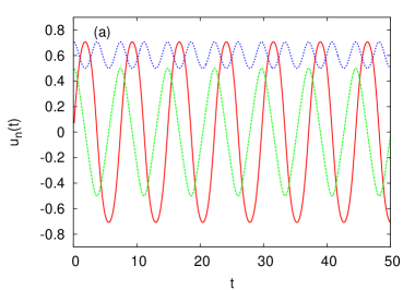
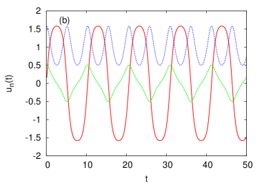
Figure 1: Plot of numerical solutions to a GOY shell model with three shells and complex amplitudes $u_{n}(t)$ in the absence of forcing and viscosity. Plotted are: $\rm{Re}~{}u_{1}(t)({\rm red}),~{}Re~{}u_{2}(t)({\rm green}),~{}Im~{}u_{3}(t)({\rm blue})$ with the initial conditions: $\rm{Re}~{}u_{1}(0)=0,~{}Im~{}u_{1}(0)=0,~{}Re~{}u_{2}(0)=0.5,~{}Im~{}u_{2}(0)=0,~{}Re~{}u_{3}(0)=0,~{}Im~{}u_{3}(0)=0.5/\sqrt{\delta}$. a): $\delta=0.5$, b): $\delta=0.1$. The curves correspond to the exact solutions Eq. (26).

It should be noted that for small $k$ the Fourier expansions in practice only contain very few terms, since $q$ is small. This also applied when $k$ is not so small. For example, if $k^{2}=\frac{1}{2}$, then $K=K^{\prime}$ and hence $q=e^{-\pi}$, so $q^{n}$ is fast decreasing. However, when $k$ approaches 1, a large number of terms are needed in the Fourier transforms because in this case $q$ is not small. This follows because $q$ can be expressed in terms of $k$ by the formula

$$q=\lambda+2\lambda^{5}+15\lambda^{9}+150\lambda^{13}+...,~{}~{}\lambda=\frac{1}{2}~{}\frac{1-(1-k^{2})^{1/4}}{1+(1-k^{2})^{1/4}}.$$ (22)

In the case $L=0$, i.e. $u_{3}(0)^{2}=(1-\delta)/\delta~{}u_{2}(0)^{2}$, the solution (9) does not give an oscillating solution any longer. Instead one obtains

$$u_{2}(t)=u_{2}(0)$$

$$\times\frac{2~{}\sqrt{u_{1}(0)^{2}+u_{2}(0)^{2}/\delta}~{}e^{-\sqrt{M\delta(1-\delta)}~{}rt}}{\sqrt{u_{1}(0)^{2}+u_{2}(0)^{2}/\delta}+u_{1}(0)+(\sqrt{u_{1}(0)^{2}+u_{2}(0)^{2}/\delta}-u_{1}(0))~{}e^{-2\sqrt{M\delta(1-\delta)}~{}rt}}.$$ (23)

In this case $k=1$, and obviously an infinite number of Fourier modes are needed to produce the exponentially decreasing behavior (23). From eq. (23) one can easily obtain $u_{1}$ by use of the conservation law and (6),

$$u_{1}(t)=\sqrt{u_{1}(0)^{2}+u_{2}(0)^{2}/\delta}$$

$$\frac{\sqrt{u_{1}(0)^{2}+u_{2}(0)^{2}/\delta}+u_{1}(0)-(\sqrt{u_{1}(0)^{2}+u_{2}(0)^{2}/\delta}-u_{1}(0))~{}e^{-2\sqrt{M\delta(1-\delta)}~{}rt}}{\sqrt{u_{1}(0)^{2}+u_{2}(0)^{2}/\delta}+u_{1}(0)+(\sqrt{u_{1}(0)^{2}+u_{2}(0)^{2}/\delta}-u_{1}(0))~{}e^{-2\sqrt{M\delta(1-\delta)}~{}rt}}.$$ (24)

Thus, at $t\rightarrow\infty$ all the energy has gone to the $u_{1}-$mode.

In three dimensions $1-\delta$ is positive, whereas in two dimension this quantity is negative. From (11) it then follows that $k^{2}>0$ in 3D, whereas $k^{2}<0$ in 2D if $|u_{3}(0)|^{2}>(\delta-1)|u_{1}(0)|^{2}$. The Jacobi elliptic functions can be continued to negative $k^{2}$, so this does not pose any problem. The continued functions are given by

$${\rm sn}(x,ik) = \frac{1}{\sqrt{1+k^{2}}}~{}\frac{{\rm sn}(x\sqrt{1+k^{2}},\frac{k}{\sqrt{1+k^{2}}})}{{\rm dn}(x\sqrt{1+k^{2}},\frac{k}{\sqrt{1+k^{2}}})},~{}~{}{\rm cn}(x,ik)=\frac{{\rm cn}(x\sqrt{1+k^{2}},\frac{k}{\sqrt{1+k^{2}}})}{{\rm dn}(x\sqrt{1+k^{2}},\frac{k}{\sqrt{1+k^{2}}})},$$

$${\rm dn}(x,ik) = \frac{1}{{\rm dn}(x\sqrt{1+k^{2}},\frac{k}{\sqrt{1+k^{2}}})}.$$ (25)

For $k\rightarrow 0\pm$ these functions are continuous.

The solutions (10)-(14) simplify if $u_{1}(0)=0$ and $u_{2}(0)^{2}/\delta=u_{3}(0)^{2}$. From (11) we see that in this case $k^{2}=1-\delta$, and

$$u_{1}(t)=i\frac{a}{\sqrt{\delta}}~{}{\rm sn}(art,\sqrt{1-\delta}),~{}~{}u_{2}(t)=a~{}{\rm cn}(art,\sqrt{1-\delta}),~{}~{}u_{3}(t)=\frac{a}{\sqrt{\delta}}~{}{\rm dn}(art,\sqrt{1-\delta}).$$ (26)

Here $a=u_{2}(0)$. In Fig. 1 we show these exact solutions by direct numerical integration of the GOY model with three shells (with specific initial conditions). Note the familiar behavior of the Jacobi elliptic functions. Two different values of the parameter $\delta$ are shown in order to vary the elliptic functions parameter $k^{2}=1-\delta$. The solutions are stable and the numerical integrations can proceed indefinitely.

We also mention that if $k=0$, corresponding to $\delta=1$, sn and cn become sin and cos, respectively, and dn approaches the constant one. From eq. (11) we see that $k^{2}=0$ if $\delta=1$. This case has been studied (including viscosity) in po .

II.2 Solution with variable phases

We shall now discuss the case of variable phases. In forming the energy or other conserved quantities they do not enter directly. However, in this section we shall see that the phases do play a dynamical role. Letting the phases be allowed to vary a new solution emerges, which can still be expressed in terms of Jacobian elliptic function, but which has one more free parameter than the solutions (10)-(14).

The three-shell model with variable phases defined by $u_{n}=|u_{n}|e^{i\phi_{n}}$ can be rewritten as six equations,

$$\frac{d|u_{1}|}{rdt}=|u_{2}||u_{3}|~{}\sin(\phi_{1}+\phi_{2}+\phi_{3}),~{}\frac{d|u_{2}|}{rdt}=-\delta|u_{1}||u_{3}|~{}\sin(\phi_{1}+\phi_{2}+\phi_{3}),$$

$${\rm and}~{}\frac{d|u_{3}|}{rdt}=-(1-\delta)|u_{2}||u_{1}|~{}\sin(\phi_{1}+\phi_{2}+\phi_{3}),$$ (27)

as well as

$$|u_{1}|~{}\frac{d\phi_{1}}{rdt}=|u_{2}||u_{3}|~{}\cos(\phi_{1}+\phi_{2}+\phi_{3}),~{}|u_{2}|~{}\frac{d\phi_{2}}{rdt}=-\delta|u_{1}||u_{3}|~{}\cos(\phi_{1}+\phi_{2}+\phi_{3}),$$

$${\rm and}~{}|u_{3}|~{}\frac{d\phi_{3}}{rdt}=-(1-\delta)|u_{1}||u_{2}|~{}\cos(\phi_{1}+\phi_{2}+\phi_{3}).$$ (28)

From the last equations we easily derive

$$\frac{d(\phi_{1}+\phi_{2}+\phi_{3})}{rdt}=-\cos(\phi_{1}+\phi_{2}+\phi_{3})~{}\left[-\frac{|u_{2}||u_{3}|}{|u_{1}|}+\delta\frac{|u_{1}||u_{3}|}{|u_{2}|}+(1-\delta)\frac{|u_{1}||u_{2}|}{|u_{3}|}\right],$$ (29)

On the left we can use eqs. (27) in the square bracket to get

$$\frac{d(\phi_{1}+\phi_{2}+\phi_{3})}{dt}=\cot(\phi_{1}+\phi_{2}+\phi_{3})~{}\frac{d\ln(|u_{1}||u_{2}||u_{3}|)}{dt},$$ (30)

from which we get

$$\cos(\phi_{1}+\phi_{2}+\phi_{3})=\frac{N}{|u_{1}||u_{2}||u_{3}|},$$ (31)

where $N$ is a constant. We see that if the phases are constants, i.e. $N=0$, their sum must be $\pi/2$ mod $\pi$ (i.e. $\pi/2,~{}3\pi/2$,…), as already used in the previous subsection.

From the cosine in (31) we can compute the sine and insert it in eqs. (27). By this procedure we arrive at

$$\frac{d|u_{1}|}{rdt}=\frac{1}{|u_{1}|}~{}\sqrt{|u_{1}|^{2}|u_{2}|^{2}|u_{3}|^{2}-N^{2}},~{}~{}\frac{d|u_{2}|}{rdt}=-\delta~{}\frac{1}{|u_{2}|}~{}\sqrt{|u_{1}|^{2}|u_{2}|^{2}|u_{3}|^{2}-N^{2}}$$

$${\rm and}~{}\frac{d|u_{3}|}{rdt}=-(1-\delta)~{}\frac{1}{|u_{3}|}~{}\sqrt{|u_{1}|^{2}|u_{2}|^{2}|u_{3}|^{2}-N^{2}}.$$ (32)

In this equation we have inserted a positive square root, corresponding to a positive sine. Since the left hand sides of the eqs. (32) can also be negative in some range of $t$ values, it follows that for such values of $t$ a negative sign should be chosen for in front of the square roots in eqs. (32), corresponding to negative values of the sine. In order not to make the notation too clumsy we do not indicate this explicitly. Further from eq. (27) we can easily derive like eqs. (5), (6)

$$|u_{3}|^{2}=L+\frac{1-\delta}{\delta}|u_{2}|^{2}~{}~{}{\rm and}~{}~{}|u_{1}|^{2}=M-\frac{1}{\delta}|u_{2}|^{2}.$$ (33)

This allows us to express any $|u_{n}|$ in terms of the other two $|u|^{\prime}$s. Using this in eqs. (32) we obtain for example for $|u_{2}|$ the equation of motion,

$$\frac{d|u_{2}|^{2}}{2\delta\sqrt{|u_{2}|^{2}(M-|u_{2}|^{2}/\delta)(L+|u_{2}|^{2}~{}(1-\delta)/\delta)-N^{2}}}=-d(rt).$$ (34)

This is again an elliptic type of integral. However, it is slightly more complicated than the solutions considered in the previous subsection.

Inside the square root we have a polynomial of third degree in $|u_{2}|^{2}$. If we introduce the zeros of this polynomial, this is the prototype of an integral which can be inverted by the use of Theta functions WW . However, instead of seeking the most general solution, in the following we shall study only a limited range of parameters corresponding to a limited range of the initial values of the $u^{\prime}$s.

To obtain a relatively simple solution we must remember that the Jacobi elliptic functions are not really independent, as is seen from eq. (15). Therefore one could attempt to make an ansatz in such a manner that inside the square root we have three squares of elliptic functions, which requires

$$|u_{1}|^{2}=A_{1}+B_{1}~{}{\rm sn}^{2}(art),~{}|u_{2}|^{2}=A_{2}+B_{2}~{}{\rm cn}^{2}(art),~{}{\rm and}~{}|u_{3}|^{2}=A_{3}+B_{3}~{}{\rm dn}^{2}(art).$$ (35)

With a suitable choice of the $A$ and $B$ constants the square root in eq. (34) could then produce the product ${\rm sn}(at)~{}{\rm cn}(at)~{}{\rm dn}(at)$ to be matched by the derivative in the numerator, $d{\rm cn}^{2}(at)=-2{\rm cn}(at)~{}{\rm sn}(at)~{}{\rm dn}(at)~{}dt$ (see eq. (16)).

Instead of proceeding from the integral (34) it is actually easier to insert the ansatz (35) directly in the equations of motion (32). This gives a number of algebraic equations. When we differentiate the functions (35) in order to insert them on the left hand sides in (32) we get a result proportional to $B_{n}~{}{\rm sn}(art)~{}{\rm cn}(art)~{}{\rm dn}(art)/|u_{n}|$ with $n=1,2,3$ by use of eqs. (16). To match the right hand sides of eqs. (32) we therefore need

$$\sqrt{|u_{1}|^{2}|u_{2}|^{2}|u_{3}|^{2}-N^{2}}\propto~{}{\rm sn}(art){\rm cn}(art){\rm dn}(art).$$ (36)

This means that the following conditions must be satisfied ,

$$aB_{1}=\sqrt{B_{1}B_{2}B_{3}},~{}~{}aB_{2}=\delta~{}\sqrt{B_{1}B_{2}B_{3}},~{}~{}k^{2}aB_{3}=(1-\delta)\sqrt{B_{1}B_{2}B_{3}}.$$ (37)

As before in eq. (26), we take $k^{2}=1-\delta$. Then the restrictions (37) are easily solved

$$B_{1}=a^{2}/\delta,~{}B_{2}=a^{2},~{}~{}B_{3}=a^{2}/\delta.$$ (38)

The remaining conditions then become

$$0=-A_{3}a^{4}/\delta-A_{2}(1-\delta)a^{4}/\delta^{2}+A_{1}(1-\delta)a^{4}/\delta,$$ (39)

which is the requirement that the coefficient of sn${}^{4}(art)$ vanish, and

$$N^{2}=A_{1}A_{2}A_{3}+A_{1}A_{3}a^{2}+A_{1}A_{2}a^{2}/\delta+A_{1}a^{4}/\delta,$$ (40)

which expresses the condition that the coefficient of sn${}^{0}(art)$ vanishes, and

$$0=A_{2}A_{3}a^{2}/\delta-A_{1}A_{3}a^{2}+A_{3}a^{4}/\delta-A_{1}A_{2}(1-\delta)a^{2}/\delta+A_{2}a^{4}/\delta^{2}-A_{1}a^{4}/\delta-A_{1}(1-\delta)a^{4}/\delta,$$ (41)

which expresses the condition that the coefficient of sn${}^{2}(art)$ vanishes.

The solutions of (39)-(41) should be such that the square root on the right hand sides of eq. (32) should be real. This is not a trivial requirement. One can study this question in general by first solving for $A_{3}$ in terms of $A_{1},A_{2}$ by use of eq. (39), and (41) then becomes a second order equation which gives $A_{2}$ in terms of $A_{1}$. In this way we obtain

$$A_{3}=(1-\delta)(A_{1}-A_{2}/\delta),$$ (42)

$$A_{2}=\frac{\delta}{2(1-\delta)}\left(a^{2}+(1-\delta)A_{1}\pm\sqrt{a^{4}+(1-\delta)A_{1}\left(2a^{2}\frac{\delta-2}{\delta}-3(1-\delta)A_{1}\right)}~{}\right),$$ (43)

as well as

$$N^{2}=A_{1}^{3}~{}\delta(1-\delta)+A_{1}^{2}a^{2}(2-\delta)+A_{1}a^{4}/\delta.$$ (44)

The last restriction can be compared to eq. (31), which expresses the constant $N$ in terms of the initial values of the phases and the $|u|^{\prime}$s. Using eq. (38) to find the initial $|u|^{\prime}$s and comparing this to eq. (44) we see that the ansatz (35) is valid only when cosine of the sum of the initial phases is equal to plus/minus one, i.e.

$$\phi_{1}(0)+\phi_{2}(0)+\phi_{3}(0)=0~{}({\rm mod}~{}\pi).$$ (45)

This does not mean that the phases at later times are restricted in this way.

The requirements (42),(43) and (44) do not give acceptable (real) results for all values of $A_{1}$ and $a$, since we need to ensure that in (44) $N^{2}>0$ and that the square root in (43) should be real. Let us therefore give a numerical example where the results are good. We have found that if $\delta=1-1/r=1/2$ (3D, with the often used value $r=2$) and $a=1$ the following values are completely consistent (the square root is real!),

$$A_{1}=0.309,~{}~{}A_{2}=0.577,~{}~{}A_{3}=-0.423,~{}~{}N^{2}=0.7685.$$ (46)

For initial values of the phases and the $|u|^{\prime}$s which are not covered by the ansatz (35) one must go back to the standard elliptic integral (34), and treat it in other ways than done here.

The solution (35) can be used to obtain an integral representation for the phases. We can insert the cosine from eq. (31) in the equations of motion for the phases (28), and we get

$$\phi_{1}(t)=\phi_{1}(0)+N~{}\int^{t}_{0}\frac{dt}{A_{1}+(a^{2}/\delta)~{}{\rm sn}^{2}(art)},$$ (47)

with similar expressions for the other phases.

It should also be mentioned that it is possible to take into account the viscosity terms in the equations for the phases. The result is

$$\frac{d\phi_{1}}{dt}=\frac{N}{|u_{1}|^{2}}~{}e^{-\nu(k_{1}^{2}+k_{2}^{2}+k_{3}^{2})t},$$ (48)

with similar expressions for the other phases. Unfortunately we have not been able to solve for the modulus $|u_{1}|$ when viscosity is included.

In conclusion we have seen that if the phases are allowed to vary, this situation gives rize to the new solutions (35). So, although the phases do not appear in the energy and other conserved quantities and one might therefore consider them unphysical, this is not true because of their dynamical importance. As the phases are allowed to vary continuously this indeed outlines an infinity of exact periodic solutions to the GOY models with three shells.

II.3 Inclusion of a constant force

We shall now consider the case where a constant force ($f$ is taken to be imaginary, $f\rightarrow if$) is included in the first shell, so that (2) reads

$$\frac{du_{1}}{dt}=ru_{2}(t)~{}u_{3}(t)+f,$$ (49)

whereas the other two equations (3) and (4) are unchanged. For this reason we derive like in eq. (5)

$$u_{3}(t)^{2}=L+\frac{1-\delta}{\delta}~{}u_{2}(t)^{2}.$$ (50)

However, eq. (6) is now replaced by

$$\frac{1}{2}~{}u_{1}(t)^{2}-f\int^{t}_{0}dt^{\prime}~{}u_{1}(t^{\prime})=\frac{1}{2}~{}M-\frac{1}{2\delta}~{}u_{2}(t)^{2}.$$ (51)

Here the initial conditions again determine the constants $M$ and $L$. The integral on the left hand side can be determined from eq. (3) and (50),

$$-r\delta~{}u_{1}=\frac{1}{u_{3}}\frac{du_{2}}{dt}=\frac{du_{2}/dt}{\sqrt{L+\frac{1-\delta}{\delta}~{}u_{2}^{2}}}.$$ (52)

Thus,

$$-r\delta~{}\int_{0}^{t}dt^{\prime}~{}u_{1}(t^{\prime})=\sqrt{\frac{\delta}{1-\delta}}~{}\ln\frac{u_{2}(t)+\sqrt{u_{2}(t)^{2}+\frac{L\delta}{1-\delta}}}{u_{2}(0)+\sqrt{u_{2}(0)^{2}+\frac{L\delta}{1-\delta}}}.$$ (53)

Inserting this in eq. (3) we obtain by use of eq. (50)

$$-r\delta~{}t=\int\frac{du_{2}}{u_{1}u_{3}}=\int_{u_{2}(0)}^{u_{2}(t)}\frac{du_{2}}{\sqrt{\left(L+\frac{1-\delta}{\delta}~{}u_{2}^{2}\right)\left(M-\frac{1}{\delta}u_{2}^{2}-f\frac{1}{r\sqrt{\delta(1-\delta)}}~{}\ln\frac{u_{2}+\sqrt{u_{2}^{2}+\frac{L\delta}{1-\delta}}}{u_{2}(0)+\sqrt{u_{2}(0)^{2}+\frac{L\delta}{1-\delta}}}~{}\right)}}.$$ (54)

This in principle expresses $u_{2}$ as a function of $t$, and $u_{1}$ can then be obtained from (51), whereas $u_{3}$ can be obtained from (50). However, due to the logarithm in the denominator we cannot use elliptic functions to invert eq. (54).

If $L=0$ and $f/r$ is large and positive, it is possible to obtain an asymptotic expression for the integral (54) by introducing the variable

$$z=M-\frac{1}{\delta}u_{2}^{2}-\frac{2f}{r\sqrt{\delta(1-\delta)}}~{}\ln\frac{u_{2}}{u_{2}(0)}.$$ (55)

By a partial integration one then obtains

$$-\sqrt{\delta(1-\delta)}~{}rt=-\int_{0}^{z_{0}}\frac{dz}{\sqrt{z}\left(2u_{2}^{2}/\delta+2f/(r\sqrt{\delta(1-\delta)}\right)}$$

$$=-\left[\frac{2\sqrt{z}}{2u_{2}^{2}/\delta+2f/(r\sqrt{\delta(1-\delta)})}\right]_{0}^{z_{0}}~{}\left(1+O\left(\frac{1}{f}\right)\right).$$ (56)

Here $z_{0}$ is obtained from the substitution (55) just by inserting the upper limit $u_{2}(t)$ instead of the integration variable $u_{2}$. With the assumption $u_{2}\ll f|\ln u_{2}|$ we can invert this expression and obtain

$$u_{2}(t)\approx u_{2}(0)~{}e^{-\sqrt{\delta(1-\delta})~{}frt^{2}/2}.$$ (57)

This expression works quite well for large $f^{\prime}$s, as one can see by solving eq. (49) numerically. Thus the assumption $u_{2}\ll f|\ln u_{2}|$ is self-consistent.

For $f<0$ we have not been able to find asymptotic results. Numerically one can easily see that in this case $u_{2}(t)$ oscillates. In the Fig. 2 we show numerical solutions of the GOY model with three shells with a small forcing added. The solutions are surprisingly still stable even though energy is now added into the system. We observe the interesting phenomenon that the dn-function undergoes a period doubling when the value of the forcing is changed. We were however not able to identify a series of period doubling eventually leading into a chaotic state.

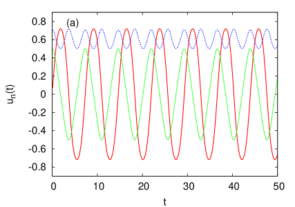
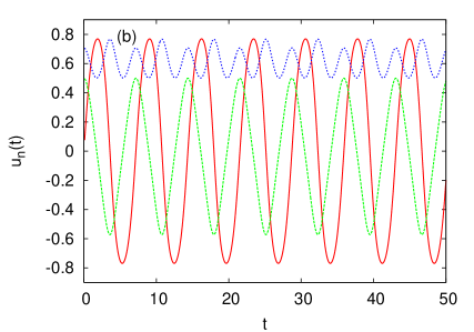
Figure 2: Plot of the Jacobi elliptic functions for three shells with addition of a force, a): $f=(1+i)\cdot 10^{-2}$ b): $f=(5+5i)\cdot 10^{-2}$ with otherwise the same values of the parameters and the same initial conditions as in Fig. 1. Note that compared to a) the variation in the dn function has undergone a period doubling. In both cases a),b) the solutions are stable.

III Many shells

In this section we shall extend one of the results obtained in the last section. We start by defining the functions

$$Ja_{1} = {\rm sn}(art+b),~{}Ja_{2}={\rm cn}(art+b),~{}Ja_{3}={\rm dn}(art+b),$$

$$Ja_{4} = {\rm sn}(art+b),~{}Ja_{5}={\rm cn}(art+b),~{}Ja_{6}={\rm dn}(art+b),$$

$$Ja_{7} = {\rm sn}(art+b),...,$$ (58)

where the symbol $Ja$ stands for Jacobi. In general $Ja_{n}=Ja_{n-3}$. The $Ja^{\prime}$s satisfy the differential equations

$$dJa_{n}/dt=\epsilon_{n}~{}Ja_{n+1}Ja_{n+2}.$$ (59)

Here

$$\epsilon_{n}=+1~{}{\rm if}~{}n=1~{}~{}({\rm mod}~{}3),~{}~{}\epsilon_{n}=-1~{}{\rm if}~{}n=2~{}~{}({\rm mod}~{}3),~{}~{}\epsilon_{n}=-k^{2}~{}{\rm if}~{}n=3~{}~{}({\rm mod}~{}3).$$ (60)

The modulus $k^{2}$ is to be determined by the requirement that the functions

$$u_{n}=A_{n}~{}Ja_{n}(art+b)$$ (61)

should satisfy the shell equations up to some order. Similarly, the constants $a,~{}b$ and $A_{n}$ should be restricted from this requirement. Eq. (61) is of course a generalization of (10), (13), and (14). As an example we show in Fig. 3 two solution to the unforced GOY model with six shells. By just changing the initial conditions in the six’th shell, the solution change from being quasiperiodic to a chaotic signal. Thus in the Hamiltonian 12-dimensional phase space stable periodic and quasiperiodic islands are situated between chaotic areas as is a well known scenario for Hamiltonian systems of low dimension.

The shell model without viscosity and forcing

$$\frac{du_{n}^{\star}}{dt}=-ik_{n}\left(u_{n+1}u_{n+2}-\frac{\delta}{r}~{}u_{n-1}u_{n+1}-\frac{1-\delta}{r^{2}}~{}u_{n-1}u_{n-2}\right).$$ (62)

is satisfied exactly by the ansatz (61), because by direct insertion we get

$${\rm LHS}=A^{\star}_{n}ar\epsilon_{n}Ja_{n+1}(at)Ja_{n+2}(at)=$$ (63)

$$-ik_{n}\left(A_{n+1}A_{n+2}Ja_{n+1}Ja_{n+2}-\frac{\delta}{r}~{}A_{n-1}A_{n+1}Ja_{n-1}Ja_{n+1}-\frac{1-\delta}{r^{2}}~{}A_{n-1}A_{n-2}Ja_{n-1}Ja_{n-2}\right),$$

and using that the $Ja^{\prime}$s are defined mod 3 in the index we get

$$Ja_{n-1}=Ja_{n+2}~{}~{}{\rm(in~{}second~{}and~{}third~{}terms)},~{}~{}Ja_{n-2}=Ja_{n+1}~{}~{}{\rm(in~{}third~{}term)}.$$ (64)

which shows that the $Ja^{\prime}$s cancel out on both sides of eq. (63). The $A^{\prime}$s should therefore satisfy

$$raA^{\star}_{n}\epsilon_{n}=-ik_{n}\left(A_{n+1}A_{n+2}-\frac{\delta}{r}A_{n-1}A_{n+1}-\frac{1-\delta}{r^{2}}A_{n-1}A_{n-2}\right).$$ (65)

This can be rewritten as a recursion relation

$$A_{n+2}=\frac{iraA_{n}^{\star}\epsilon_{n}}{k_{n}A_{n+1}}+\frac{\delta}{r}~{}A_{n-1}+\frac{1-\delta}{r^{2}}~{}\frac{A_{n-1}A_{n-2}}{A_{n+1}}.$$ (66)

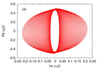
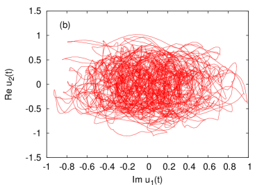
Figure 3: Numerical solutions of the unforced GOY model six shells. The initial conditions are: a): $\rm{Re}~{}u_{1}(0)=~{}1.2,~{}Im~{}u_{1}(0)=0.6,~{}Re~{}u_{2}=0.5,~{}Im~{}u_{2}(0)=0.9,~{}Re~{}u_{3}=0.5,~{}Im~{}u_{3}(0)=2.0,~{}Re~{}u_{4}(0)=0.0,~{}Im~{}u_{4}(0)=0.707,~{}Re~{}u_{5}=0.0,~{}Im~{}u_{5}=.5,~{}Re~{}u_{6}=0.0,~{}Im~{}u_{6}=8.0$. The solution is given by a stable quasiperiodic trajectory. b): $\rm{Re}~{}u_{1}(0)=1.2,~{}Im~{}u_{1}(0)=0.6,~{}Re~{}u_{2}=0.5,~{}Im~{}u_{2}(0)=0.9,~{}Re~{}u_{3}=0.5,~{}Im~{}u_{3}(0)=2.0,~{}Re~{}u_{4}(0)=0.0,~{}Im~{}u_{4}(0)=0.707,~{}Re~{}u_{5}=0.0,~{}Im~{}u_{5}=.5,~{}Re~{}u_{6}=0.0,~{}Im~{}u_{6}=0.5$. By just changing the initial condition for $\rm{Im}~{}u_{6}$, the solution changes from a quasiperiodic into a chaotic trajectory.

We have not succeeded in showing that this relation always has a solution. However, it is instructive to compare to the results in the last section. Let us start to solve the recursion relation (66),

$$A_{3}=\frac{iaA_{1}^{\star}}{A_{2}},$$ (67)

$$A_{4}=\frac{1}{rA_{1}^{\star}}~{}\left(\delta|A_{1}|^{2}-|A_{2}|^{2}\right),$$ (68)

and

$$A_{5}=\frac{1}{rA_{2}^{\star}(\delta|A_{1}|^{2}-|A_{2}|^{2})}~{}\left(-k^{2}a^{2}|A_{1}|^{2}+(\delta^{2}-\delta+1)~{}|A_{1}|^{2}|A_{2}|^{2}-\delta~{}|A_{2}|^{4}\right).$$ (69)

Subsequent coefficients get more complex. The next one is

$$A_{6}=\frac{ia(A_{4}^{\star}+r(1-\delta)A_{1}^{\star})}{r^{3}A_{5}}+\frac{ia\delta A_{1}^{\star}}{rA_{2}},$$ (70)

Here eqs. (68) and (69) should be inserted.

To gain some insight in the recursion scheme let us start by assuming that there are only three shells. Then we should require that $A_{4}=0$, i.e. from (68)

$$|A_{2}|=\sqrt{\delta}~{}|A_{1}|.$$ (71)

Further, from the requirement $A_{5}A_{4}=0$ one obtains

$$0=-k^{2}a^{2}|A_{1}|^{2}+(\delta^{2}-\delta+1)~{}|A_{1}|^{2}|A_{2}|^{2}-\delta~{}|A_{2}|^{4}.$$ (72)

Inserting (71) this gives

$$k^{2}=(1-\delta)\frac{|A_{2}|^{2}}{a^{2}},$$ (73)

which is exactly the same as the previously obtained result (11).

We mention that usually the GOY model is just truncated at some shell number, in this case $n=3$. However, in dealing with the analytic solutions this is absolutely necessary since we need the information contained when the two subsequent shell amplitudes (in this case $n=$4 and 5) are put equal to zero, leading to a value for $k^{2}$, which shows that only the first amplitude is a free parameter. Therefore it is necessary to proceed in the somewhat unconventional way followed above, also when we consider an arbitrary but finite number of shells, as we shall see in the following.

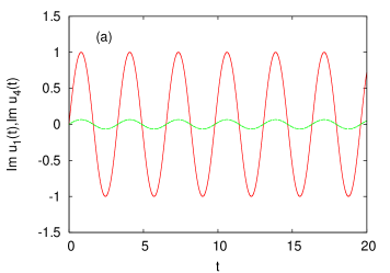
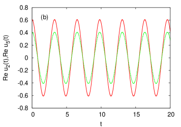
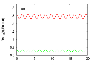
Figure 4: The solutions to the GOY model with six shells without forcing and viscosity for $\delta=0.5$ with the following scaling coefficients: $\alpha_{4}=0.06527718351453,~{}~{}~{}\alpha_{5}=0.6704413705072,~{}~{}~{}\alpha_{6}=0.44861490325181$ and parameter values $a=1,b=0,A_{1}=1$. This leads to the following initial values: $\rm{Re}~{}u_{1}(0)=~{}Im~{}u_{1}(0)=~{}Im~{}u_{2}(0)=~{}Im~{}u_{3}(0)=~{}Re~{}u_{4}(0)=~{}Im~{}u_{4}(0)=~{}Im~{}u_{5}(0)=~{}Im~{}u_{6}(0)=0.0,~{}Re~{}u_{2}(0)=0.607820697,~{}Re~{}u_{3}(0)=1.645222028,~{}Re~{}u_{5}(0)=0.407507916,~{}Re~{}u_{6}(0)=0.73807128$. The following shell model variables are plotted: a): $\rm{Im}~{}u_{1}(t),~{}\rm{Im}~{}u_{4}(t)$; b): $\rm{Re}~{}u_{2}(t),~{}\rm{Re}~{}u_{5}(t)$; c): $\rm{Re}~{}u_{3}(t),~{}\rm{Re}~{}u_{6}(t)$.

With six shells we need

$$A_{7}=0=\frac{-iaA_{5}^{\star}}{r^{4}A_{6}}+\frac{\delta}{r}A_{4}+\frac{1-\delta}{r^{2}}\frac{iaA_{1}^{\star}A_{4}}{A_{2}A_{6}},$$ (74)

and

$$A_{7}A_{8}=0=-\frac{iak^{2}A_{6}^{\star}}{r^{5}}+\frac{(1-\delta)}{r^{2}}~{}A_{5}A_{4}.$$ (75)

Eqs. (74) and (75) can in principle be used to determine $k^{2}$. The algebra is, however, quite involved.

It is possible to simplify the rather tedious algebra by introducing the following ansatz,

$$A_{4}=\alpha_{4}~{}A_{1},~{}~{}A_{5}=\alpha_{5}~{}A_{2},~{}{\rm and}~{}~{}A_{6}=\alpha_{6}~{}A_{3}.$$ (76)

Here we have assigned $A_{1}$ and $A_{4}$ the phase $\pi/2$, whereas the other $A^{\prime}$s are real. In the following, we take all the $A_{i}^{\prime}$s to be real. From eq. (68) we see that

$$A_{2}^{2}=(\delta-r\alpha_{4})~{}A_{1}^{2}.$$ (77)

From eq. (69) we similarly get

$$k^{2}=\left(-r^{2}\alpha_{4}~{}\alpha_{5}+1-\delta+r\delta\alpha_{4}\right)~{}\frac{A_{2}^{2}}{a^{2}}.$$ (78)

Next we consider the recursion relation (70) for $A_{6}$ which gives

$$\alpha_{6}=\frac{\alpha_{4}+r(1-\delta)}{r^{3}\alpha_{5}}+\frac{\delta}{r}.$$ (79)

The conditions for the shell model to stop at six shells are represented by eqs. (74) and (75), which lead to

$$\frac{\delta}{r}~{}\alpha_{4}~{}\alpha_{6}=\frac{\alpha_{5}}{r^{4}}~{}\left(\delta-r\alpha_{4}\right)-\frac{1-\delta}{r^{2}}~{}\alpha_{4},$$ (80)

and

$$(1-\delta)~{}\alpha_{4}~{}\alpha_{5}=\frac{\alpha_{6}}{r^{3}}~{}\left(-r^{2}\alpha_{4}\alpha_{5}+1-\delta+r\delta~{}\alpha_{4}\right),$$ (81)

respectively. In the last equation we used $k^{2}$ from eq. (78).

From these three equations we can obtain the three $\alpha^{\prime}$s in terms of the parameters $r,\delta$. This elimination procedure leads to a sixth order equation for $\alpha_{4}$, and from the solutions of this equation the other $\alpha^{\prime}$s can then be obtained.

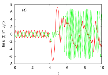
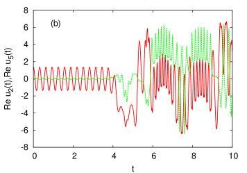
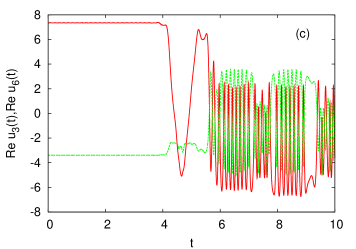
Figure 5: The solutions to the GOY model with six shells without forcing and viscosity for $\delta=0.5$. We apply the following scaling coefficients: $\alpha_{4}=-0.6788645691146,~{}~{}~{}\alpha_{5}=-0.05642693495529,~{}~{}~{}\alpha_{6}=-0.46139658555751$. Setting $a=10,b=0,A_{1}=1$ give the following initial conditions: $\rm{Re}~{}u_{1}(0)=~{}Im~{}u_{1}(0)=~{}Im~{}u_{2}(0)=~{}Im~{}u_{3}(0)=~{}Re~{}u_{4}(0)=~{}Im~{}u_{4}(0)=Im~{}u_{5}=~{}Im~{}u_{6}=0.0,~{}Re~{}u_{2}=1.362985377,~{}Re~{}u_{3}=7.33683587,~{}Re~{}u_{5}=-0.076909087,~{}Re~{}u_{6}=-3.385191019$

This procedure leads to extremely messy expressions which are not useful, since we do not have analytic solutions of sixth order equations. Instead, it is much simpler to assign numerical values for the parameters. Taking $r=2$ and $\delta=1/2$ (3D) we obtain from eqs. (79), (80) and (81) by use of NSolve in Mathematica (applied to these three simultaneous equations) the following real solutions:

$$\alpha_{4}=0.06527718351453,~{}~{}~{}\alpha_{5}=0.6704413705072,~{}~{}~{}\alpha_{6}=0.44861490325181$$

$$\alpha_{4}=-0.6788645691146,~{}~{}~{}\alpha_{5}=-0.05642693495529,~{}~{}~{}\alpha_{6}=-0.46139658555751,$$

$$\alpha_{4}=-17.345971520666,~{}~{}~{}\alpha_{5}=1.3995954432919,~{}~{}~{}\alpha_{6}=-1.2098836041347,$$

$${\rm Not~{}acceptable~{}(see~{}remark~{}below~{}eq.~{}}(\ref{sas})):$$

$$\alpha_{4}=0.625261,~{}~{}~{}\alpha_{5}=-0.309106,~{}~{}~{}\alpha_{6}=-0.407242$$ (82)

From eq. (77) there are relations between $A_{1}$ and $A_{2}$, and using the numbers in (82) we get

$$A_{2}^{2}/A_{1}^{2}=\delta-r\alpha_{4}=0.369446,~{}~{}1.85773,~{}~{}35.1919,$$ (83)

respectively. Here the fourth line in eq. (82) has been ignored, since it does not lead to a real ratio $A_{2}/A_{1}$, as assumed in the above derivation. Thus there only three acceptable solutions.

For $k^{2}$ we obtain

$$\frac{k^{2}a^{2}}{A_{2}^{2}}=80.2634,~{}~{}~{}-0.33209,~{}~{}~{}0.390219,$$ (84)

respectively.

In Figs. 4,5 we show two of the exact solutions to the model GOY with six shells as given in (82) by the first two set of $\alpha_{n}$-values. In the first case, shown in Fig. 4, we obtain the familiar Jacobi elliptic function with the exact relationships between the amplitude as predicted by the theory. Notice that the amplitude of Im $u_{1}$ come to exactly 1 even though the initial condition of the mode is set to zero. These solutions are stable. In Fig. 5 we show the the second analytic solution in (82). Note we here have set the frequency to $a=10$ in order to obtain a value of the elliptic parameter $k$ less than one. In this case, again, the numerical integrations starts out tracing out the exact analytical solutions in terms of Jacobi elliptic functions. However, as is clear from Fig. 5 these solutions are unstable since after some time they turn into chaotic trajectories. We have experimented numerically with the accuracy of the $\alpha_{n}$ coefficients and the accuracy of the integration. As is expected, for unstable solutions in a chaotic “sea”, the exact solution can be sustained numerically longer the higher the accuracy.

The GOY model has been modified by changing the order of the complex conjugates of the velocity amplitudes resulting in the Sabra model sabra1 . We have checked that the Jacobi elliptic functions are also exact solutions to this model. One can derive recursion relations like eqs. (79),(80),(81) which have a similar structure but the conjugations and a sign appear differently. This is discussed in some details in Appendix B.

In order to study the stability of the solutions further, we have initiated the integration with the exact solutions shown in Fig. 4 but with the addition of a small force. As is seen form the simulation (shown in Fig. 6), the solution starts out to be stable, looking very similar to the exact solution, however in the long run also become unstable and chaotic. Nevertheless, we have observed numerically that the existence of this transition depends very much on the value of the added forcing $f$. For some values of $f$, the solutions remain stable although slightly changed away from the exact solutions. For other values of $f$ we observe the scenario depicted in Fig. 6. We shall not elaborate further on these transitions in the present paper.

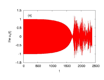
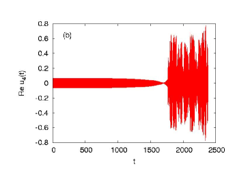
Figure 6: Solutions to the GOY model with six shells and with the same parameter values as in Fig. 4 but with addition of a small forcing $\rm{Re}{\it f}=\rm{Im}{\it f}=0.001$. Note that the solutions appear to be stable for a long time but turn into chaotic trajectories eventually. Plotted are: a) $\rm{Re}~{}u_{1}(t)$; b): $\rm{Re}~{}u_{4}(t)$.

It is well known for the GOY shell model that at the parameter value $\delta=1.25$ the enstrophy $H=\sum_{n=1}^{N}k_{n}^{2}|u_{n}|^{2}$ is a conserved quantity. This point therefore corresponds to two-dimensional turbulence with a forward cascade of enstrophy and an inverse cascade of energy mogens . We have therefore also looked for exact solutions to the GOY model with six shells at this point and by using $r=2$ and $\delta=1.25$ we obtain as before from eqs. (79), (80) and (81) by use of NSolve in Mathematica the following real solutions:

$$\alpha_{4}=0.289785,~{}~{}~{}\alpha_{5}=2.21803,~{}~{}~{}\alpha_{6}=0.613153$$

$$\alpha_{4}=-0.108771,~{}~{}~{}\alpha_{5}=0.112449,~{}~{}~{}\alpha_{6}=-0.0517172,$$

$$\alpha_{4}=0.0856125,~{}~{}~{}\alpha_{5}=0.160463,~{}~{}~{}\alpha_{6}=0.302194,$$

$$\alpha_{4}=0.0982932,~{}~{}~{}\alpha_{5}=0.359568,~{}~{}~{}\alpha_{6}=0.485351$$ (85)

with the following relations between the amplitudes $A_{2}$ and $A_{1}$

$$A_{2}^{2}/A_{1}^{2}=0.67043,1.46754,1.07878,1.05341$$ (86)

and the elliptic parameter $k$ determined by:

$$k^{2}a^{2}/A_{2}^{2}=-4.9655,-0.473003,-0.0909193,-0.145639$$ (87)

Of these four solutions to the 2D analogy for turbulence we have found numerically that number one, three and four on the list are unstable whereas number two is stable. As examples of this we show in Fig. 7 some of the solutions, the ones corresponding to the second and the fourth in the list. As compared to the 3D case, we observe that the solutions in Fig. 7b become unstable even faster and that they clearly behave very chaotically.

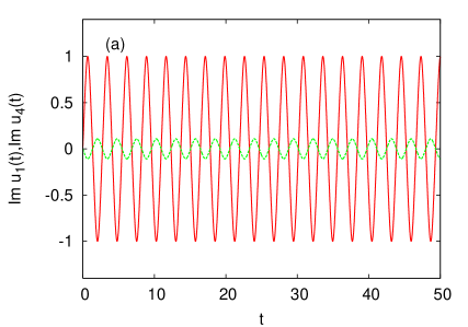
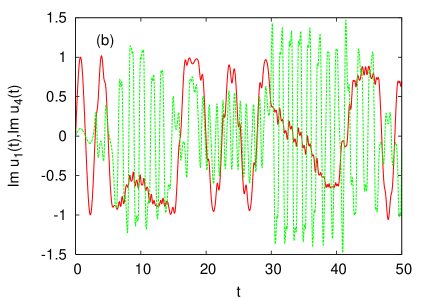
Figure 7: Plot of the Jacobi elliptic functions for six shells for the case of $\delta=1.25$ for enstrophy conservation corresponding to 2D turbulence for two different sets of $\alpha_{n}$ values from (85) (the initial conditions are adjusted accordingly). a): $\alpha_{4}=-0.108771,~{}~{}~{}\alpha_{5}=0.112449,~{}~{}~{}\alpha_{6}=-0.0517172$. Here the solutions in terms of elliptic functions are stable. b): $\alpha_{4}=0.0982932,~{}~{}~{}\alpha_{5}=0.359568,~{}~{}~{}\alpha_{6}=0.485351$. The solutions ’follow’ the elliptic solutions for a few periods and the clearly become unstable.

In Appendix A, we present solutions for the case of nine shells. Furthermore, we derive a general recursion relation which allows to solve the $\alpha_{n}$ coefficients for any number of shells. If the number of shell goes to infinity one can see from these recursion relations that the only scaling law solution behaves like $\alpha_{n}\sim k_{n}^{-\frac{1}{3}}$ as expected from the Kolmogorov theory mogens .

We end this section by pointing out that the solutions based on the ansatz (76) are special. Presumably the general recursion relations (66) for the amplitudes of the Jacobi functions can have more general solutions, where the constant phases could also enter the recursions. In any case, the solutions that we found represent an infinite set of solutions, since the continuous parameters $A_{1},~{}A_{2},~{}a,~{}b$ can vary freely. Alternatively, an analysis of eqs. (61), (66) shows that the free parameters are $u_{1}(0),u_{2}(0),u_{3}(0)$ and $A_{1}$. Since these quantities in general are complex, this represents an $\infty^{8}$-continuous set of parameters.

IV Conclusions

We have derived a series of exact analytical solutions to the GOY shell model in the absence of forcing and viscosity. In this model a shell couples to nearest and next-nearest neighbor shells and the very construction of these couplings directly suggest that the solutions should be formulated in terms of Jacobi elliptic functions. We have presented closed form Jacobi solutions in the case of three shells at which point the GOY model is completely integrable and possesses a continuous infinity of stable solutions. We have further derived exact recursion relations for the amplitudes of the elliptic functions in case of 6, 9, 12 etc shells which is related to the period three symmetry of the GOY model. Some of these solutions are stable and others are unstable. In the last cases the trajectories lie on chaotic energy surfaces. This picture of an infinity of solutions, some either periodic or quasi-periodic and others chaotic is common for Hamiltonian systems where the trajectories will move on surfaces of constant energy. Our results therefore complement the picture presented for the GOY model with forcing and viscosity obtained in GOYper where long periodic unstable solutions are found embedded in the large dimensional phase space of the dynamics of a GOY model with many shells. In this limit of many shells we have found solutions that behave according to the Kolmogorov scaling theory for energy spectra, which shows the physical relevance of our periodic solutions. Indeed, we have also observed that adding a small force, thus destroying the Hamiltonian property of the system, changes the solutions. Some of them are destabilized but some might remain periodic even when a force is added. The case of a forced GOY model is closer to a realistic system for turbulence and it is for future research to investigate how our solutions might be relevant for a turbulent state when a true energy cascade over many scales is present.

Acknowledgments

We are very grateful for discussions with Leo Kadanoff on shell models with few shells, which initiated this work. Also we really appreciate the many very constructive comments by Bruno Eckhardt.

Appendix A: Solutions with nine shells

In this appendix we shall discuss the case of nine shells. Following the same procedure as in the main text we obtain (the equations for $n<7$ are the same as before, but for completeness we include the $n=6$ eq. (79) below):

$$\alpha_{6}=\frac{\alpha_{4}+r(1-\delta)}{r^{3}\alpha_{5}}+\frac{\delta}{r}.$$ (88)

$$\alpha_{7}=-\frac{\alpha_{5}}{r^{4}\alpha_{6}}~{}(\delta-r\alpha_{4})+\frac{\delta}{r}\alpha_{4}+\frac{(1-\delta)~{}\alpha_{4}}{r^{2}\alpha_{6}},$$ (89)

and

$$\alpha_{8}=-(-r^{2}\alpha_{4}\alpha_{5}+1-\delta+r\delta\alpha_{4})\frac{\alpha_{6}}{r^{5}\alpha_{7}}+\frac{\delta}{r}\alpha_{5}+\frac{1-\delta}{r^{2}\alpha_{7}}~{}\alpha_{5}\alpha_{4},$$ (90)

and

$$\alpha_{9}=\frac{\alpha_{7}}{r^{6}\alpha_{8}}+\frac{\delta}{r}\alpha_{6}+\frac{1-\delta}{r^{2}\alpha_{8}}\alpha_{5}\alpha_{6},$$ (91)

and

$$\frac{\delta}{r}~{}\alpha_{7}\alpha_{9}=\frac{\alpha_{8}}{r^{7}}~{}(\delta-r\alpha_{4})-\frac{1-\delta}{r^{2}}~{}\alpha_{7}\alpha_{6},$$ (92)

as well as

$$(1-\delta)\alpha_{7}\alpha_{8}=\frac{\alpha_{9}}{r^{6}}~{}(-r^{2}\alpha_{4}\alpha_{5}+1-\delta+r\delta\alpha_{4}).$$ (93)

These coupled equations can be solved using the simple Mathematica program ($\delta=.5,r=2$)

$${\rm NSolve}[\{z==(x+1)/(2^{3}y)+1/4,r==-y(1/2-2x)/(2^{4}z)+1/4x+1/2^{3}x/z,$$

$$s==-(-4xy+1/2+x)z/(2^{5}r)+1/4y+1/2^{3}xy/r,$$

$$t==r/(2^{6}s)+1/4z+1/2^{3}yz/s,1/4rt==s/2^{7}(1/2-2x)-1/2^{3}zr,$$

$$1/2rs==t/2^{6}(-4xy+1/2+x)\},\{x,y,z,r,s,t\}],$$ (94)

where the notation is

$$\alpha_{4}=x,~{}\alpha_{5}=y,~{}\alpha_{6}=z,~{}\alpha_{7}=r,~{}\alpha_{8}=s,~{}\alpha_{9}=t,$$ (95)

One obtains 32 solutions, some of which are complex, and some which leads to $A_{2}^{2}<0$. Only seven of these solutions are acceptable. The reader who is interested in the actual numbers should just run the above program. Increased accuracy can be obtained by putting $,d$ at the end of the square bracket in (94), where $d$ is the number of wanted decimals.

For the $\alpha^{\prime}$s we can also obtain in general recursion relations by use of eq. (66). Defining $A_{n}=\alpha_{n}A_{1}$ if $n=4$ mod(3),$A_{n}=\alpha_{n}A_{2}$ if $n=5$ mod(3) and $A_{n}=\alpha_{n}A_{3}$ if $n=6$ mod(3), we obtain for $n\geq 4$

$$\alpha_{n+2}=\frac{\tilde{\epsilon}_{n}\alpha_{n}}{r^{n-1}\alpha_{n+1}}+\frac{\delta}{r}~{}\alpha_{n-1}+\frac{1-\delta}{r^{2}}~{}\frac{\alpha_{n-1}\alpha_{n-2}}{\alpha_{n+1}},$$ (96)

where we defined $\alpha_{1}=\alpha_{2}=\alpha_{3}=1$. Here ($n=0,1,2,3,...$)

$$\tilde{\epsilon}_{4+3n}=1,~{}\tilde{\epsilon}_{5+3n}=-(\delta-r\alpha_{4}),~{}\tilde{\epsilon}_{6+3n}=-(1-\delta+r\delta\alpha_{4}-r^{2}\alpha_{4}\alpha_{5}).$$ (97)

In addition there are two “stop-equations”: Suppose we stop at the number of shells $=3N$, then we must satisfy that $A_{3N+1}=0$ and $A_{3N+1}A_{3N+2}=0$, which lead to the two equations

$$\delta~{}\alpha_{3N-2}\alpha_{3N}=\frac{\alpha_{3N-1}}{r^{3N-3}}~{}(\delta-r\alpha_{4})-\frac{1-\delta}{r}~{}\alpha_{3N-3}\alpha_{3N-2},$$ (98)

and

$$(1-\delta)~{}\alpha_{3N-2}\alpha_{3N-1}=\frac{\alpha_{3N}}{r^{3N-3}}~{}(1-\delta+r\delta\alpha_{4}-r^{2}\alpha_{4}\alpha_{5}).$$ (99)

By means of eqs. (96), (98) and (99) it is easy to write down the relevant equations for any number of shells. The remaining problem is the numerical solution of these equations. We are not able to show the existence of acceptable solutions in general, but have checked that they exist for six and nine shells.

In case with an infinite number of shells, $N\to\infty$, the “stop-equations” (98) and (99) should of course not be applied so we are left only with eq. (96). If we make the ansatz $\alpha_{n}\sim r^{\beta_{n}}$, then the only solution is

$$\beta_{n}=-\frac{n}{3}~{}~{},$$ (100)

which is fully consistent with the Kolmogorov theory for turbulence. The first term in Eq. (96) is totally subdominant with this ansatz.

Appendix B: Solutions to the Sabra model

In this appendix we shall derive results similar to those in Section III for the Sabra-model sabra1 . This model is given by

$$\dot{u}_{n}=ir^{n}\left[u_{n+1}^{\star}u_{n+2}-\frac{\delta}{r}u_{n-1}^{\star}u_{n+1}+\frac{1-\delta}{r^{2}}u_{n-1}u_{n-2}\right].$$ (101)

We can now easily check that if the ansatz (61) is inserted in this equation, like in the GOY model, the Jacobi functions cancel on both sides and we are left with the following recursion relation

$$A_{n+2}=-\frac{ia\epsilon_{n}A_{n}}{r^{n-1}A^{\star}_{n+1}}+\frac{\delta}{r}~{}A^{\star}_{n-1}~{}\frac{A_{n+1}}{A^{\star}_{n+1}}-\frac{1-\delta}{r^{2}}~{}\frac{A_{n-1}A_{n-2}}{A_{n+1}^{\star}}.$$ (102)

This is the Sabra-version of the analogous GOY model equation (66). We can then proceed to solve for the first few $A^{\prime}$s,

$$A_{3}=-\frac{iaA_{1}}{A_{2}^{\star}},$$ (103)

which is similar to eq. (67),

$$A_{4}=-\frac{A_{2}}{rA_{1}^{\star}A_{2}^{\star}}~{}\left(\delta|A_{1}|^{2}-|A_{2}|^{2}\right),$$ (104)

similar to eq. (68), and

$$A_{5}=\frac{A_{1}^{2}A_{2}}{r(A_{2}^{\star})^{2}|A_{1}|^{2}(\delta|A_{1}|^{2}-|A_{2}|^{2})}\left[-a^{2}k^{2}|A_{1}|^{2}+(\delta^{2}-\delta+1)|A_{1}|^{2}|A_{2}|^{2}+\delta|A_{2}|^{4}\right],$$ (105)

which is similar to eq. (69). One can of course continue like in Section III to obtain further equations from the general recursion relation (102).

For the case of three shells we should again require that $A_{4}=0$, which gives

$$|A_{2}|^{2}=\delta|A_{1}|^{2}.$$ (106)

Requiring further that $A_{5}A_{4}=0$, we obtain

$$a^{2}k^{2}=(1-\delta)~{}|A_{2}|^{2}.$$ (107)

Eqs. (106) and (107) are completely the same as the analogous equations obtained in the GOY model in Section III. However, in the case of more shells this is certainly not expected to continue.

References

- (1) Bohr T, Jensen MH, Paladin G and Vulpiani A 1998 “Dynamical systems approach to turbulence”, Cambridge University Press, Cambridge.
- (2) Bowman JC, Doering CR, Eckhardt B, Davoudi J Roberts M and Schumacher J 2006 Links between dissipation, intermittency, and helicity in the GOY model revisited Physica D 218, 1
- (3) Carbone V and Veltri P 1992 Relaxation processes in magnetohydrodynamics: a triad-interaction model Astron. Astrophys. 259, 359-372
- (4) Christiansen F, Cvitanovic P and Putkaradze V 1997 Spatiotemporal chaos in terms of unstable recurrent patterns Nonlinearity 10, 55.
- (5) Cvitanovic P and Eckhardt B 1991 Periodic orbit expansion for classical smooth flows J. Phys. A 24, L237-41
- (6) Eckhardt B, Schneider TM, Hof B and Westerweel J 2007 Turbulent Transition in Pipe Flow Annu. Rev. Fluid Mech. 39, 447-68.
- (7) Frisch U 1995 “Turbulence: The legacy of A.N. Kolmogorov”, Cambridge University Press.
- (8) Frisch U, She ZS and Thual O 1986 Viscoelastic behaviour of cellular solutions to the Kuramoto-Sivashinsky model J. Fluid Mech. 168, 221.
- (9) Gledzer EB 1973 System of hydrodynamic type admitting two quadratic integrals of motion Sov. Phys. Dokl. 18, 216.
- (10) Jensen MH, Paladin G and Vulpiani A 1991 Intermittency in a cascade model for three-dimensional turbulence Phys. Rev. A 43, 798.
- (11) Kadanoff LP, Lohse D, Wang J and Benzi R 1995 Scaling and Dissipation in the GOY shell model Phys. Fluids 7, 617.
- (12) Kadanoff LP, Lohse D and Schörghofer N 1997 Scaling and linear response in the GOY turbulence model Physica D 100, 165.
- (13) Kato S and Yamada M 2003 Unstable periodic solutions embedded in a shell model turbulence Phys. Rev. E 68, 025302(R).
- (14) Kawahara G and Kida 2001 Periodic motion embedded in plane Couette turbulence: regeneration cycle and burst Jour. Fluid Mech., 449, 291-300
- (15) Kawahara G, Kida S and van Veen L 2006 Unstable periodic motion in turbulent flows Nonlin. Proc. in Geophys. 13, 499-507
- (16) L’vov VS, Podivilov E, Pomyalov A, Procaccia I and Vandembrouq D 1998 Improved shell model of turbulence Phys. Rev. E 58, 1811.
- (17) L’vov VS 2002 Quasisolitons and asymptotic multiscaling in shell models of turbulence Phys. Rev. E 65, 026309
- (18) Olesen P 2007 On the zero viscosity limit arXiv:hep-th/0701237
- (19) Toh S and Itano T 2003 A periodic-like solution in channel flow J. Fluid. Mech. 481, 67-76
- (20) van Veen L, Kida S and Kawahara G 2006 Periodic motion representing isotropic turbulence Fluid Dynamics Res. 38, 19-46
- (21) Waleffe F 2001 Exact coherent structures in channel flow J. Fluid. Mech. 435, 93-102
- (22) Whittaker ET and Watson GN 1902, A course of modern analysis, Cambridge University Press, Cambridge.
- (23) Yamada M and Ohkitani K 1987 Lyapunov Spectrum of a Chaotic Model of Three-Dimensional Turbulence J. Phys. Soc. Japan 56, 4210-4213; Yamada M and Ohkitani K 1988 The Inertial Subrange and Non-Positive Lyapunov Exponents in Fully-Developed Turbulence Prog. Theor. Phys. 79,1265-1268.