Time-dependent analytic solutions of quasi-steady shocks with cooling

Abstract

I present time-dependent analytical solutions of quasi-steady shocks with cooling, where quasi-steady shocks are objects composed of truncated steady-state models of shocks at any intermediate time. I compare these solutions to simulations with a hydrodynamical code and finally discuss quasi-steady shocks as approximations to time-dependent shocks. Large departure of both the adiabatic and steady-state approximations from the quasi-steady solution emphasise the importance of the cooling history in determining the trajectory of a shock.

Keywords: analytic solutions ; time-dependent ; shocks ; cooling

1 Introduction

Analytic solutions of well defined problems are often used as benchmark tests for hydrodynamical codes. However, the most widely used tests such as the Sedov blast wave (Sedov, 1993) or the Sod shock tube test (Sod, 1978) are almost all adiabatic or with Mach numbers of order unity. By contrast, gas in astrophysical contexts can be subject to strong cooling and Mach numbers of order a few hundreds are common place in protostellar jets. There is hence a lack of analytical solutions with cooling or at high Mach numbers. I present here time-dependent analytical solutions of quasi-steady shocks with cooling for arbitrarily high Mach numbers.

Lesaffre et al. (2004a) and Lesaffre et al. (2004b) studied the temporal evolution of molecular shocks and found that they are most of the time in a quasi-steady state, ie: an intermediate time snapshot is composed of truncated steady state models. They showed that if the solution to the steady state problem is known for a range of parameters, it is possible to compute the time-dependent evolution of quasi-steady shocks by just solving an implicit ordinary differential equation (ODE). Since the steady state problem is itself an ODE, it is very easy to numerically compute the temporal evolution of quasi-steady shocks.

However, a given cooling function of the gas does not necessarily lead to an analytical steady state solution. Furthermore, even when it does, the implicit ODE which drives the shock trajectory does not necessarily have an analytical solution itself. In this paper, we tackle the problem in its middle part : we assume a functional form for the steady state solutions (section 2). We then show how to recover the underlying cooling function that yields these steady states (section 3). Finally, we exhibit a case where the shock trajectory has an analytical solution (section 4) and we compare it to numerical simulations (section 5). Results are discussed in section 6 and conclusions drawn in section 7.

2 Method

Consider the following experimental set up: we throw gas with a given pressure, density and supersonic speed $v_{0}$ on a wall. We assume a perfect equation of state with adiabatic index $\gamma$. We assume the net rate of cooling of the gas is a function $\Lambda(\rho,p)$ where $p$ and $\rho$ are the local density and pressure of the gas. The gas is shocked upon hitting the wall, heated up by viscous friction and an adiabatic shock front develops that soon detaches from the wall. Behind this front, the gas progressively cools down towards a new thermal equilibrium state and a relaxation layer unrolls.

All physical quantities are normalised using the entrance values of pressure and density, so that the sound speed of the unshocked gas is $c_{0}=\sqrt{\gamma}$. The time and length scales will be later specified by the cooling time scale (see section 3.1).

Consider now the set of all possible stationary states for the velocity profile in the frame of the shock front. A given entrance speed $u_{0}$ in the shock front provides the velocity $u$ at a given distance $y$ behind the shock front:

$$u=f(y,u_{0})\mbox{.}$$ (1)

The adiabatic jump conditions for an infinitely thin (or steady) shock enforce $f(0,u_{0})=u_{a}(u_{0})$ where

$$u_{a}(u_{0})=\frac{\gamma-1}{\gamma+1}u_{0}+\frac{2\gamma}{\gamma+1}\frac{1}{u_{0}}\mbox{.}$$ (2)

Unfortunately, that $f$ is a simple algebraic function of $y$ and $u_{0}$ does not necessarily imply an algebraic form for $\Lambda(\rho,p)$. It is in fact more appropriate to express $y$ in terms of $u$ and $u_{0}$. We hence rather write (1) in the following manner:

$$y=g(u,u_{0})$$ (3)

with the condition

$$g(u_{a},u_{0})=0\mbox{.}$$ (4)

Section 3.1 details how to recover $\Lambda(\rho,p)$ from $g(u,u_{0})$.

Lesaffre et al. (2004b) provide the ODE for the evolution of the distance from the shock to the wall $r$ with respect to time $t$ if the shock is quasi-steady at all times:

$$\dot{r}=f(r,\dot{r}+v_{0})$$ (5)

where a dot denotes a derivative with respect to time. This equation can also be expressed with the function $g$:

$$r=g(\dot{r},\dot{r}+v_{0})\mbox{.}$$ (6)

In section 4 I show how one can integrate equation (6) and give an analytical expression for a simple form of $g$. In section 5 I compare this solution to a time-dependent numerical simulation.

3 Cooling function

3.1 General procedure

Let us write the equation of steady-state hydrodynamics in the frame of the shock with entrance parameters $(\rho,p,u)=(1,1,u_{0})$:

$$\rho u=u_{0}\mbox{,}$$ (7)

$$p+\rho u^{2}=1+u_{0}^{2}$$ (8)

and

$$\frac{\partial}{\partial y}[u(\frac{\gamma}{\gamma-1}p+\frac{1}{2}\rho u^{2})]=\Lambda$$ (9)

with the boundary condition $u=u_{a}(u_{0})$ at $y=0$.

One can solve the equations (7) and (8) for $\rho$ and $p$ and use the relations into (9) which becomes:

$$\Lambda(u,y,u_{0})=\frac{\partial}{\partial y}[u(\frac{\gamma}{\gamma-1}(1-uu_{0}+u_{0}^{2})+\frac{1}{2}uu_{0})]$$ (10)

Expansion of the derivative with respect to $y$ provides:

$$\Lambda(u,u^{\prime},u_{0})=\frac{\gamma}{\gamma-1}(1+u_{0}^{2})u^{\prime}-\frac{\gamma+1}{\gamma-1}u_{0}uu^{\prime}$$ (11)

where $u^{\prime}={\partial u}/{\partial y}$.

By taking the derivative of equation (3) we easily extract $u^{\prime}$ in terms of $u$ and $u_{0}$:

$$u^{\prime}=1/\frac{\partial g}{\partial u}(u,u_{0})\mbox{.}$$ (12)

(12) combined with (11) provides $\Lambda(u,u_{0})$. (7) and (8) finally give $\Lambda(\rho,p)$.

3.2 First application

I now illustrate this method with a simple function $g(u,u_{0})$. In a typical radiative shock in the interstellar medium, the post-shock gas finally cools down to nearly the same temperature as the pre-shock gas. To mimic this effect, we need a cooling function such that its thermal equilibrium is the isothermal state. In other words, $\Lambda(\rho,p)=0$ implies $\rho=p$. This is equivalent to asking that the final steady velocity of any shock verifies the isothermal jump condition $u=u_{i}$ where $u_{i}(u_{0})=1/u_{0}$:

$$\lim_{u\rightarrow u_{i}}\frac{\partial g}{\partial u}(u,u_{0})=-\infty\mbox{.}$$ (13)

To verify both conditions (4) and (13) we take the simple form:

$$g(u,u_{0})=\beta\frac{u_{a}(u_{0})-u}{u-u_{i}(u_{0})}$$ (14)

where $\beta>0$ determines the strength of the cooling. Setting a length scale allows to assume $\beta=1$. The above procedure (section 3.1) yields:

$$\Lambda(p,\rho)=-\frac{1}{\beta}\left(\frac{\left(1+\gamma\right)\,\left[1+p\,\left(\gamma\,\rho-\gamma-1\right)\right]\,{\left(p-\rho\right)}^{2}}{{\left(\gamma-1\right)}^{2}\,{\left(\rho-1\right)}^{\frac{3}{2}}\,\left(p\,\rho-1\right)\,\sqrt{\rho\,\left(p-1\right)}}\right)$$ (15)

This cooling function is displayed on figure 1. In addition to the temperature $T=p/\rho=1$ solution, the thermal equilibrium state $\Lambda(p,\rho)=0$ is also realised when the factor $\left[1+p\,\left(\gamma\,\rho-\gamma-1\right)\right]$ is set to zero. However, this state is practically never achieved in the relaxation layer of a shock as it happens for densities $\rho<1+1/\gamma$ and $\rho$ is always greater than the adiabatic compression factor $C_{a}=(\gamma+1)/(\gamma-1+2\gamma u_{0}^{-2})\simeq 1+2/(\gamma-1)$ for strong shocks. In the high temperature limit $\Lambda$ scales like $T^{\frac{3}{2}}$ which is reminiscent of the collisional coupling between gas and dust for low dust temperatures. But in the high density limit, $\Lambda\simeq\rho^{-\frac{1}{2}}T^{\frac{3}{2}}$ which yields a rather unphysical scaling on the density. In the next subsection, I show how to improve the physical relevance of the cooling function, at the loss of the analytical integrability of the trajectory.

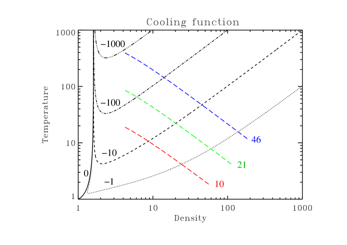
Figure 1: Contour plot of the cooling function $\Lambda$ defined by equation (15) for $\beta=1$ and $\gamma=5/3$ with respect to temperature $T=p/\rho$ and density $\rho$. Levels for the contours are 0 (solid line) and respectively -1, -10, -10² and, -10³ for dotted, dashed, dash-dotted and dash-dot-dot-dotted lines. Overlayed (long-dash) are three typical shock thermal profiles at age $t=100$ (from bottom to top $v_{0}=10$, 21 and 46).

3.3 Second application

In this section, I briefly illustrate how one can obtain semi-analytic approximation of shocks for any kind of cooling function. I start with a given cooling function $\Lambda_{0}$ and compute an analytical approximation to the steady state function $g(u,u_{0})$. I then recover the underlying cooling function $\Lambda_{1}$ for this approximate steady state and check how $\Lambda_{1}$ and $\Lambda_{0}$ differ.

A very common form for the cooling due to a collisionally excited (unsaturated) line is

$$\Lambda_{0}=-\frac{1}{\beta}\rho^{2}\exp[{-T_{0}/T}]$$ (16)

where $T_{0}$ is the temperature of the transition and $\beta$ scales the strength of the cooling. I use $\beta=1$ for simplification (it amounts to specify a length scale without loss of generality).

If we apply the procedure of section 3.1 backwards we have to integrate

$$\frac{{\rm d}y}{{\rm d}u}=\frac{u^{2}\left[\gamma(1+u_{0}^{2})-(1+\gamma)uu_{0}\right]}{(\gamma-1)\,u_{0}^{2}}\,\exp[{\frac{T_{0}\,u_{0}}{u\,(1+u_{0}^{2}-u\,u_{0})}}]$$ (17)

to find the equation for the stationary velocity profile. This equation does not have an analytical solution. But there are many approximations to the right hand side that will allow to treat the problem.

For example, we can simplify (17) by using the strong shock approximation $u_{0}>>1$ along with the high compression approximation $u>>u_{0}$:

$$\frac{{\rm d}y}{{\rm d}u}=\frac{\gamma u^{2}}{\gamma-1}\,\exp[{\frac{T_{0}}{u\,u_{0}}}]\mbox{.}$$ (18)

This equation still does not have an analytical solution but we can add a term to the factor of the exponential to get the derivative of the simple function $G(u,u_{0})=u^{4}\exp[{T_{0}}/(u\,u_{0})]$. Hence we finally take

$$\frac{{\rm d}y}{{\rm d}u}=(1-4\frac{u\,u_{0}}{T_{0}})\frac{\gamma u^{2}}{\gamma-1}\,\exp[{\frac{T_{0}}{u\,u_{0}}}]$$ (19)

which will be a good approximation provided that $T_{0}>>u_{0}^{2}$. This yields the simple form $G(u,u_{0})-G(u_{a},u_{0})$ for the function $g(u,u_{0})$ with which equation (6) can then be integrated numerically and tabulated to get a fast access to the shock trajectory.

To check that the above approximations did not alter too much the underlying cooling function, we can apply the procedure 3.1 to the simplified equation (19). This provides:

$$\Lambda_{1}(\rho,p)=-\frac{T_{0}\left[1+p\,\left(\gamma\,\rho-\gamma-1\right)\right](\rho-1)\rho}{\gamma(p-1)[4-4p+T_{0}(\rho-1)]}\exp[{-\frac{T_{0}(\rho-1)}{p-1}}]$$ (20)

Figure 2 compares contour plots of both cooling functions $\Lambda_{0}$ and $\Lambda_{1}$ (for $T_{0}=1000$ and $\gamma=5/3$). It can be seen that despite the crude approximations we made, $\Lambda_{0}$ and $\Lambda_{1}$ are still close to one another for a very large range of parameters (for $1<T<<T_{0}$ and $\rho>>1$ both expressions asymptotically converge). However, thermal equilibrium solutions (solid lines in figure 2) appear for $\Lambda_{1}$ when none existed for $\Lambda_{0}$. Also, the range of applicable entrance velocities is restricted to conditions such that the maximum temperature in the shock is low compared to $T_{0}$ (because we made the $T_{0}>>u_{0}^{2}$ approximation).

This is nevertheless a good illustration of this method which can in theory be applied to any cooling function. Indeed, one can in principle use the fact that $u/u_{0}$ is bounded by a constant number strictly lower than 1 to uniformly approach equation (17) with polynomials (or any other functional form simple to integrate). One then recovers an analytical expression for $g(u,u_{0})$ arbitrary close to the exact solution.

Figure 2: Contour plot of the cooling functions $\Lambda_{0}$ and $\Lambda_{1}$ for $\beta=1$, $T_{0}=1000$ and $\gamma=5/3$ with respect to temperature $T=p/\rho$ and density $\rho$. Levels for the contours are 0 (solid line, only for $\Lambda_{1}$) and -10², -1, -10^-2, -10^-4 and -10^-6 from top to bottom for dotted ($\Lambda_{0}$) and dashed ($\Lambda_{1}$) lines.

4 Shock trajectory

4.1 Exact solution

Implicit ODEs like (6) are in principle straightforward to integrate numerically. It is however much harder to find an analytically integrable form for these equations. Such a solution nevertheless exists for the simple but physically relevant example (14).

Let us use (14) into (6) with $\beta=1$ to obtain

$$r=\frac{2\gamma+(\gamma-1)v_{0}^{2}+(\gamma-3)\,\dot{r}\,v_{0}}{(\gamma+1)\,(\dot{r}^{2}+\dot{r}\,v_{0}-1)}$$ (21)

The solution of (21) for $\dot{r}$ yields only one positive root $\dot{r}=h(r)$:

$$h(r)=\frac{(\gamma-3)\,v_{0}-(\gamma+1)v_{0}\,r+s(r)}{2(\gamma+1)\,r}$$ (22)

where

$$s(r)=\sqrt{a+b\,r+c\,r^{2}}$$ (23)

with

$$a=(\gamma-3)^{2}\,v_{0}^{2}\mbox{ ,}$$ (24)

$$b=2(\gamma+1)[4\,\gamma+(\gamma+1)\,v_{0}^{2}]$$ (25)

and

$$c=(\gamma+1)^{2}(4+v_{0}^{2})\mbox{.}$$ (26)

We are hence able to express the age $t$ of the shock as a function of its position $r$ which provides the trajectory:

$$t(r)=\int_{0}^{r}\frac{{\rm d}x}{h(x)}$$ (27)

We now write $1/h(x)$ as a sum of integrable terms:

$$\frac{1}{h(x)}=\frac{1}{2}v_{0}+\frac{b+2c\,x}{4(\gamma+1)\,s(x)}+\frac{e}{2s(x)}-\frac{d}{2(z+x)}+\frac{(\gamma+1)\,d^{2}}{2(z+x)\,s(x)}$$ (28)

with

$$d=\frac{\gamma-1}{\gamma+1}v_{0}(3+v_{0}^{2})\mbox{ ,}$$ (29)

$$e=4\gamma+5(\gamma-1)v_{0}^{2}+(\gamma-1)\,v_{0}^{4}$$ (30)

and

$$z=\frac{2\gamma}{\gamma+1}+\frac{\gamma-1}{\gamma+1}v_{0}^{2}\mbox{.}$$ (31)

We then integrate expression (28) to obtain the trajectory in its final analytical form

$$t(r)=\frac{v_{0}}{2}r+\frac{s(r)-\sqrt{a}}{2(\gamma+1)}+\frac{e}{2\sqrt{c}}\log\left(\frac{b+2\sqrt{a\,c}}{b+2c\,r+2\sqrt{c}\,s(r)}\right)+\frac{d}{2}\log\left(\frac{z}{z+r}\right)$$

$$+\frac{(\gamma+1)\,d^{2}}{2s(-z)}\log\left(\frac{(z+r)(2a-b\,z+2\sqrt{a}\,s(-z))}{z[(2a-b\,z)+(b-2c\,z)r+2s(r)s(-z)]}\right)$$ (32)

If $r(t)$ is wanted, $t(r)$ can be numerically inverted by a Newton method of zero finding. This is done easily since the derivative $t^{\prime}(r)=1/h(r)$ is provided analytically.

4.2 High Mach number approximation

We can recover a more simple but approximate trajectory if we make two assumptions :

• in the limit of high Mach numbers ($v_{0}/c_{0}\rightarrow\infty$), the adiabatic compression factor becomes a constant:

  $$u_{a}(u_{0})\simeq\frac{\gamma-1}{\gamma+1}u_{0}\mbox{.}$$ (33)

• at late times, the compression factor is nearly the isothermal compression factor and $\dot{r}\simeq 1/u_{0}$. Hence for high Mach numbers $u_{0}=v_{0}+\dot{r}\simeq v_{0}$ and we use:

  $$u_{i}(u_{0})\simeq 1/v_{0}$$ (34)

With both these approximations, (14) with $\beta=1$ becomes

$$g(u,u_{0})=v_{0}\frac{(1-\gamma)\,u_{0}+(\gamma+1)\,u}{(\gamma+1)\,(u\,v_{0}-1)}\mbox{ ,}$$ (35)

the shock front velocity is:

$$h(r)=\frac{(\gamma-1)\,v_{0}^{2}+(\gamma+1)\,r}{v_{0}\,[2+(\gamma+1)\,r]}$$ (36)

and the resulting trajectory is

$$t(r)=v_{0}\,r+v_{0}\,(\frac{\gamma-1}{\gamma+1}v_{0}^{2}-\frac{2}{\gamma+1})\log\left(\frac{(\gamma-1)\,v_{0}^{2}}{(\gamma-1)\,v_{0}^{2}+(\gamma+1)\,r}\right)\mbox{.}$$ (37)

For early times (small $r$) the strong adiabatic shock trajectory is recovered:

$$t(r)\simeq\frac{2}{\gamma-1}\frac{r}{v_{0}}\mbox{.}$$ (38)

For very late times (very large $r$) the isothermal shock trajectory is reached asymptotically:

$$t(r)\simeq v_{0}\,r\mbox{.}$$ (39)

5 Numerical simulation

5.1 Numerical method

I compute here the time evolution of a radiative shock with cooling function (15) thanks to a 1D hydrodynamical code. This code makes use of a moving grid algorithm (Dorfi & Drury, 1987) which greatly helps to resolve the adiabatic front while keeping the total number of zones fixed to 100. The mesh driving function (see Dorfi & Drury, 1987) is designed to resolve the temperature gradients.

The advection scheme is upwind, Donnor-Cell. The time integration is implicit fully non-linear with an implicitation parameter of 0.55 as a compromise between stability and accuracy. The time-step control keeps the sum of the absolute values of the variations of all variables lower than 0.5. In practice, the maximum variation of individual variables at each time-step is lower than 1%.

I use a viscous pressure of the form:

$$p_{v}=\frac{4}{3}\rho c_{s}\sqrt{(\Delta x/10)^{2}+l^{2}}\max(-\frac{\partial u}{\partial x},0)$$ (40)

where $c_{s}=\sqrt{\gamma p/\rho}$ is the local sound speed, $\Delta x$ is the local grid spacing and $l=10^{-3}$ is a prescribed dissipation length.

To avoid numerical difficulties due to the form of $\Lambda(\rho,p)$ when $p$ or $\rho$ are close to 1, we set $\Lambda$ to zero when $p-1$ or $\rho-1$ are lower than 10^-3. The time normalisation is such that $\beta=1$.

The entrance parameters are set to $(\rho,p,v_{0})=(1,1,10)$ with $\gamma=5/3$ and the evolution is computed until a stationary state is nearly reached.

5.2 Trajectory

The position of the shock at each time-step is computed as the position of the maximum of the ratio $p_{v}/p$ along the simulation box. I compare this trajectory to the analytical expression (32) on figure 3. At a given position, the relative difference on the ages of the shock is maximum at the very beginning, when the shock front is being formed and the position is still no more than a few dissipative lengths. For times greater than $5\times 10^{-3}$, the relative error is less than 8%, with a secondary maximum at $r\simeq 1$. An estimate for this error is given in section 6.1. Note that both the isothermal (39) and the adiabatic (38) approximations are wrong by an order of magnitude at this point. The adiabatic approximation is accurate to a 20% level only for ages lower than 0.1. Afterward the effects of cooling slow down the shock and the adiabatic solution overestimate the position by large. The isothermal approximation is valid up to a 20% level only for times greater than 3000. This is because it does not take into account the period of early times when the shock is moving swiftly and since the isothermal shock moves at a slow pace it takes time to recover the delay. In other words, the cooling history of the shock does make a difference to its position. Since the ratio between the adiabatic speed and the isothermal speed scales like $v_{0}^{2}$ this situation will be even worse for stronger shocks. By contrast, the error estimate given in section 6.1 suggests that the quasi-steady approximation is equally good for stronger shocks.

The approximate trajectory for high Mach number quasi-steady shocks (37) is also shown. It is already a very good approximation even for the relatively low Mach number ($v_{0}/c_{0}=7.75$) I use. Indeed in section 4.2 I neglected only terms of order greater than 2 in the inverse of the Mach number.

Figure 3: Trajectory of the shock age vs position in the simulation (solid) compared to the analytic expression for a quasi-steady shock (dashed) and the high Mach number approximation (dotted). Also shown (solid curve in upper pannel) is the relative error between the solid and dashed curves as well as the estimate $\ddot{r}t^{2}/r$ for this error given in section 6.1 (dotted curve in upper pannel).

5.3 Snapshots

I output the results of the simulations at a few selected time-steps. For each of these snapshots, I determine the position $r$ of the shock with $p_{v}/p$ as in the previous subsection 5.2. I then compute the velocity of the quasi-steady shock front $\dot{r}=h(r)$ thanks to (22). $u_{0}=v_{0}+\dot{r}$ gives the entrance velocity in the frame of the steady shock. I now recover the relation $u=f(y,u_{0})$ thanks to equations (3) and (14):

$$u=\frac{-2\gamma+(1-\gamma)\,u_{0}^{2}+(\gamma+1)y}{(\gamma+1)\,u_{0}(y-1)}\mbox{.}$$ (41)

The temperature ($T=p/\rho$) profile can finally be retrieved from this velocity profile thanks to the relations (7) and (8).

I compare the quasi-steady state solution to the results of the numerical simulation on figure 4. The gas is flowing from the right onto the wall on the left. At early times, when the shock front is still close to the wall, the temperature at the wall is higher in the simulation than in the quasi-steady shock. This is mainly due to the wall heating effect, which decreases at later times when the cooling function has a stronger influence on the temperature. The decrease of the maximum temperature in the shock is due to the decrease of the relative entrance velocity of the gas in the adiabatic shock front (see figure 4). Note the high resolution provided by the moving mesh at the adiabatic shock front. For later times at the end of the relaxation layer, the temperature decreases toward its final value of $T=1$ at equilibrium.

The dotted curves in figure 4 are the high Mach number solutions (see section 4.2). They already are very close to the exact solutions as the approximation is of order 2.

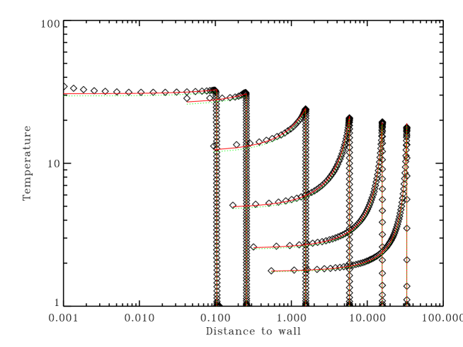
Figure 4: Temperature ($T=p/\rho$) profiles in the hydrodynamical simulation (diamonds) compared to the analytical solution for a quasi-steady shock (solid red line) and its high Mach number approximation (dotted green line).

6 Discussion

6.1 Time-dependent shocks

The differences between the quasi-steady state and the numerical solution described in section 5 both come from the numerical errors in the scheme and from the fact that quasi-steady shocks are only an approximation to time-dependent shocks. I give here an estimate on the difference between quasi-steady shocks and shocks.

I now write the inviscid equations of time-dependent hydrodynamics that a time-dependent shock would set to zero:

$$E_{\rho}=\frac{\partial\rho}{\partial t}+\frac{\partial(\rho\,v)}{\partial x}\mbox{ ,}$$ (42)

$$E_{v}=\frac{\partial v}{\partial t}+v\,\frac{\partial v}{\partial x}+\frac{1}{\rho}\,\frac{\partial p}{\partial x}$$ (43)

and

$$E_{p}=\frac{1}{(\gamma-1)}\,\frac{\partial p}{\partial t}+\frac{1}{(\gamma-1)}\,\frac{\partial(p\,v)}{\partial x}+p\,\frac{\partial v}{\partial x}-\Lambda(\rho,p)$$ (44)

where $\rho(x,t)$, $v(x,t)$ and $p(x,t)$ are the density, velocity and pressure fields in the frame of the wall.

If we now use the quasi-steady solutions to express these equations, we find

$$E_{\rho}=\frac{\partial\rho_{s}}{\partial u_{0}}\,\ddot{r}\mbox{ ,}$$ (45)

$$E_{v}=(\frac{\partial u_{s}}{\partial u_{0}}-1)\,\ddot{r}$$ (46)

and

$$E_{p}=\frac{1}{(\gamma-1)}\frac{\partial p_{s}}{\partial u_{0}}\,\ddot{r}$$ (47)

where $\rho_{s}(y,u_{0})$, $u_{s}(y,u_{0})$ and $p_{s}(y,u_{0})$ are the solutions of the steady state equations in the frame of the shock.

Hence quasi-steady shocks are in general only approximations to time-dependent shocks. The quasi-steady state approximation amounts to neglecting the acceleration $\ddot{r}$ of the shock front. Note that a maximum departure of the trajectory from the numerical simulation occurs around $r\simeq 1$ when the shock switches from adiabatic velocities to isothermal velocities (see figure 3), ie: when accelerations are likely to be the highest. A rough estimate for the relative error on the position is hence $\ddot{r}t^{2}/r$ which overestimates the error by more than about a factor 3 (see figure 3). Interestingly, this estimate does not depend on the shock velocity for strong shocks.

It is also interesting to note from equations (45)-(47) that a high dependence of the steady state on the entrance velocity $u_{0}$ will cause departures of time-dependent shocks from the quasi-steady state. In this context, refer to Lesaffre et al. (2004b) who found that the quasi-steady state was violated for marginally dissociative shocks. For this type of shocks, the entrance velocity is indeed close to the critical velocity at which the major cooling agent is dissociated and a small variation of the entrance velocity can strongly affect the post-shock.

6.2 Entrance parameters

In section 3, I used a normalisation based on the entrance values for the density and pressure: this must not hide the fact that the cooling function (15) implicitly depends on these parameters. Hence for a given cooling function, I computed analytical solutions only for a fixed set of entrance density and pressure. At this point, there is no reason why other sets of parameters should provide integrable solutions.

7 Summary and future prospects

I described a general way of obtaining time-dependent analytical solutions to quasi-steady shocks with cooling. I applied this method to a physically sensible example and compared the resulting quasi-steady shock to a time-dependent hydrodynamic simulation. I also provided a more simple high Mach number approximation to the exact solution. I showed that even though quasi-steady shocks are not strictly speaking time-dependent shocks, they are a good approximation to time-dependent shocks. In particular, more simple approximations such as the adiabatic approximation or the steady-state approximation badly fail to reproduce the behaviour of the shock for a large range of times. This is because the cooling history of the shock is essential in determining the position of the shock.

I wish to emphasise also that the method described in section 3.1 allows to recover the underlying cooling function for any set of steady state solutions. The associated quasi-steady shocks can then be easily computed by solving the ODE (6). As demonstrated in subsection 3.3 one can fit any given cooling function with analytical forms for the functions $g(u,u_{0})$. This hence provides a potentially powerful method to quickly compute the evolution of any quasi-steady shock with cooling.

Analytical solutions of quasi-steady shocks can be used as a basis to study properties of time-dependent shocks. Linear analysis around the quasi-steady solution may provide insight for the time-dependent behaviour of shocks. They can also help to address under what conditions shocks tend toward the quasi-steady state.

Furthermore, this work represents a first step towards exact solutions or better approximations to time-dependent problems of non-adiabatic hydrodynamics. In the future this might lead to new algorithms for dissipative hydrodynamical simulations. Finally, note that similar procedures can be applied to shocks with chemistry and magnetic fields (using the results of Lesaffre et al., 2004b).

References

- Dorfi & Drury (1987) Dorfi, E.A., Drury, L.O’C., Simple adaptive grids for 1-D initial value problems. J. Comput. Phys., 1987, 69, 175-195.
- Lesaffre et al. (2004a) Lesaffre, P., Chièze, J.-P., Cabrit, S., Pineau des Forêts, G., Temporal evolution of magnetic molecular shocks - I. Moving grid simulations. Astron. Astrophys., 2004a, 427, 147-156.
- Lesaffre et al. (2004b) Lesaffre, P., Chièze, J.-P., Cabrit, S., Pineau des Forêts, G., Temporal evolution of magnetic molecular shocks - II. Analytics of the steady state and semi-analytical construction of intermediate ages. Astron. Astrophys., 2004b, 427, 157-167.
- Sedov (1993) Sedov, L.I., Similarity and Dimensional Methods in Mechanics (Boca Raton: CRC Press), 10th ed., 1993
- Sod (1978) Sod, G., A survey of several finite difference methods for systems of nonlinear hyperbolic conservation laws. J. Comput. Phys., 1978, 27, 1-31.