K-Bounce
Abstract
By demanding that a bounce is nonsingular and that perturbations are well-behaved at all times, we narrow the scope of possible models with one degree of freedom that can describe a bounce in the absence of spatial curvature. We compute the general properties of the transfer matrix of perturbations through the bounce, and show that spectral distortions of the Bardeen potential are generically produced only for the small wavelengths, although the spectrum of long wavelength curvature perturbations produced in a contracting phase gets propagated unaffected through such a bounce.
1 Introduction
It has become generally admitted, especially with the recent WMAP data [1], that the Universe must have undergone a phase of inflation [2], i.e. a very short period of time during which the ongoing expansion was exponentially accelerated. This phase not only solves the usual cosmological flatness, homogeneity, monopole excess and horizon problems, but it also produces, as a bonus, an almost scale-invariant (usually, but not always, slightly red) spectrum of primordial scalar perturbations. These small inhomogeneities, of one part in about , have the right spectrum and can be given, with some amount of fine-tuning, the right amplitude to seed the large scale structure formation. In fact, it can be argued [3] that the inflationary expansion and the ensuing superadiabatic amplification of the zero-point energy of the quantum fields is the only plausible mechanism to transfer microscopic quantum fluctuations up to the cosmologically relevant length scales without annihilating the amplitudes of those fluctuations in an ever expanding universe.
Bouncing models [4, 5] have been proposed as alternatives to this scenario, mostly in the framework of string theory [6, 7] (see, however, Ref. [8]). A bounce, i.e. a period of contraction followed by expansion, could explain the flatness if the expansion phase lasted much less than the contracting era; it could explain homogeneity by making the past light cone very large during the contracting era so thermalization could take place; and, as it turns out, it can very easily give rise to the same mechanism of superadiabatic amplification as inflation [9].
The main distinction of bouncing models compared to inflation lies in which term dominates the spacetime curvature . Whereas in inflation and the physical wavelengths grow much faster than the curvature radius , close to a bounce and the curvature radius grows to as the contraction rate grinds to a halt, then falls back down rapidly as the expansion phase begins.
This means that the modes of interest are pushed inside the curvature radius during the bounce, and then out again as the universe expands. This “in-out” transition is what makes superadiabatic amplification possible, both in inflation as well as in bouncing models. The question is whether sufficiently natural models can be found which give rise to near-scale invariant spectra of cosmological perturbations [9].
As opposed to inflation, in which the phenomenological consequences of the simplest single-field, slow-roll models are extremely similar (slightly red spectra), in bouncing models the ensuing spectrum of cosmological perturbations can vary dramatically, depending on the model. Moreover, making the universe bounce is far from straightforward since general relativity forbids this behavior as long as the Null Energy Condition (NEC) holds. As a result, bouncing models can become rather intricate. The simplest bouncing models developed so far have relied on a combination of fluids [10], the presence of spatial curvature [12] or ghost fields [13]. Some models predict mode mixing with or without spectral modifications through the bounce itself, and it has been suggested that these features essentially originate from either the mixture of two fluids, i.e. from the entropy perturbations (see [10] and, in particular, [11] where the precise treatment of entropy perturbations is done), or from spatial curvature [12]. Hence the need for a single field flat space bouncing model.
Therefore, we propose here a minimalistic model for a bounce with a single matter component (a generalized scalar field, or K-essence) and zero spatial curvature. The condition that spatial curvature is small shortly after the bounce is a natural one if the contracting phase lasted much longer than the ongoing expansion phase. We also demand that the energy density is positive at all times, that a non-singular bounce takes place, and that the sound speed of perturbations is well-behaved at all times.
By expressing the Lagrangian of the generalized scalar field as a Taylor series around the field and its momenta, we can easily implement these constraints and proceed to construct a very general class of sensible bouncing models with a single fluid and no spatial curvature. The only shortcoming of our class of models is that, because near the bounce, they all lie in the “phantom” sector, , so the connection with an expanding radiation era would necessitate the introduction of matter fields and a decay mechanism similar to preheating [14]. This is precisely the scenario recently proposed in Ref. [15], where an explicit scenario is realized using the ghost condensate model [16]. For additional context on the use of non-canonical scalar fields in cosmology, see, e.g., Ref. [17, 18, 19]. Note also that if one assumes a contracting phase dominated by normal matter (preferably pressureless matter, in order to get an almost scale invariant spectrum of perturbations [20]), then because the phantom divide cannot so easily be crossed [21], there must also exist a transition between this contraction and our K-bounce, equivalent to preheating but in the other way, that one could henceforth call precooling.
The advantage of our models lies in the simplicity of their perturbative sector. We show explicitly that cosmological perturbations can be propagated in a non-singular way through the bounce. We also show that the perturbations are well-behaved through the numerous instantaneous de Sitter phases (moments of time at which ) that take place in our model.
We have computed the transfer function for perturbations, and we show that an initial spectrum of cosmological perturbations can get distorted by the bounce. As this distortion depends on the duration of the bounce, our conclusion is that bouncing models generate power spectra with a wide variety of scale dependences. However, the scale dependence of the transfer matrix is important only for short wavelengths, so that the cosmologically relevant (large) scales are transferred through the bounce unaffected.
This paper is organized as follows. First, we describe the K-essence model generating the K-bounce, provide the relevant equations of motion for the background and derive the conditions under which a bounce is possible (Sec. II). We then specify, in Sec. III, through a Taylor expansion around the bounce, the form of the pressure function we use afterwards, and provide the constraints for a non-singular bounce to take place. Sec. IV discusses a number of specific background models and attempts at classifying them by the bounce duration. We then move on, starting in Sec. V, to the study of the perturbations. We first reduce the overall system to a single equation for the only degree of freedom avalaible, which we chose to be the Bardeen gravitational potential . We discuss analytically several potentially problematic cases (the bounce itself, the instantaneous de Sitter phase, and the quasi de Sitter bounce), and we show that is well behaved at all times. Having shown the propagation of linear perturbations across the bounce to be regular at all times, we then compute numerically this time evolution, setting initial conditions at an arbitrary time at which we impose and for the Fourier modes. We end up with some considerations about model building in a concluding section.
2 Generalized scalar-field models
We will assume that the matter sector is represented by a scalar field Lagrangian of the form
| (1) |
where
| (2) |
and use the timelike signature, for the metric . From this Lagrangian, one gets a stress-energy tensor reading
| (3) |
with energy density and . These relations give back the usual one for the canonical scalar field theory provided one then takes the simplest Lagrangian function .
Since Ostrogradski’s theorem [22, 23, 24] precludes local higher derivative terms from appearing in the action principle, Eq. (1) is the most generic scalar field Lagrangian which may be stable. Notice that our Lagrangian does not need to be separable in terms of functions of the kinetic term and the field , as is sometimes assumed for K-inflation [26] or K-essence [27].
The important aspect of the quantum instability of this theory would also need to be addressed, since evidently any Hamiltonian which is unbounded from below would be instantly destroyed by quantum tunelling of positive-energy particles into the negative-energy particles [24]. For theories with non-canonical kinetic terms the quantum stability is a nontrivial issue, in particular for the case of “phantom” models – see, for instance, Ref. [21].
Introducing the flat Friedman-Lemaître-Robertson-Walker metric with scale factor , namely
and the Hubble parameter (a dot standing for a derivative w.r.t. the time coordinate ), the Einstein field equations are then given by
| (4) | |||||
| (5) |
As for the matter field, the Euler-Lagrange equation stemming from Lagrangian (1) is nothing but the conservation of the stress-energy tensor (3), i.e.
| (6) |
which, under the assumption of homogeneity of the scalar field, , is reduced to the simpler form,
| (7) |
which reduces to the Klein-Gordon equation for the canonical theory . Here the sound speed is given by
| (8) |
and it should be clear from the unapproximated equation of motion that it is the function responsible for the speed with which inhomogeneous scalar field fluctuations propagate through spacetime. In particular, a negative would give rise to exponentially growing small-scale fluctuations, meaning that the theory is classically unstable.
Since our final aim concerns the predictability and spectrum of cosmological perturbations before and after the bounce in a one-fluid model, our first requirement is that the sound speed never becomes negative. We also demand that it remains finite, since a diverging sound speed would cause a singularity in the transfer matrix [12, 13] that relates the cosmological perturbations before and after the bounce – destroying, once again, the predictability of the theory. Therefore, our first physical constraint is
| (9) |
Notice that even though we demand that the sound speed squared is always positive and finite, we should still work under the assumption that our models are just phenomenological realizations of some unknown fundamental theory, so that the second-quantized perturbations of the gravitational degrees of freedom are not being taken into account properly here. Otherwise, since both and are negative through the bounce phase in our models, the theory can become unstable, decaying instantaneously through graviton production [24, 28].
Our second requirement is that the energy is non-negative. In particular, if the bounce happens at we must have that
| (10) |
and, as a result of the Einstein equations written in the form , we conclude that we must impose
| (11) |
This means that, as , the equation of state parameter becomes infinitely negative. But is the domain of the so-called “phantom” (or “ghost”) models, and it has been shown that crossing the “ barrier” is impossible in simple single-field models [21, 29]. Therefore, our bouncing model is limited to , which in practice means that in the asymptotic past (future) the Universe approaches a contracting (expanding) de Sitter stage. These limiting stages must somehow be connected with non-phantom dominated epochs through precooling and preheating phases.
3 Taylor expansion of the Lagrangian
Our model relies on a series expansion of the Lagrangian in terms of the field and its momentum. Without loss of generality we set the value of the field at the bounce to be , and its time derivative , so we can write
In order to obtain a well-behaved bounce, it is helpful to assume that the behavior of the field near the bounce is analytic in time
| (13) |
which means that . We stress that the Taylor expansion in Eq. (13) is not used in any way to constrain the dynamics – we only use it as a means to adjust the parameters of the Lagrangian in light of the constraints.
The constraint that translates into
| (14) |
A second constraint comes from the stress tensor conservation, i.e. , imposing that at the bounce. This means that only the term in which is quadratic in time survives. In terms of our parameters, this condition is expressed as
| (15) |
Finally, the Friedman equation at leads to the third constraint, namely that and , with given by
| (16) |
Notice that and must be chosen such that the square root is real, and such that is negative. Notice also that the and branches are identified by simultaneously changing the signs of and .
To summarize: our set of constraints determines some relationships between the Lagrangian parameters , and in the context of the class of models in which the behavior of the scalar field near the bounce can be represented as Taylor series. Presumably, other models for which the scalar field around the bounce cannot be represented by such a series will lead to similar constraints between the parameters involved in these cases. As we are interested in some minimalistic bouncing model and the general conclusions that can be drawn thereof, this will suffice for us.
Notice that the scalar field parameters are essentially free, and that the Lagrangian parameters , and are also essentially free – we only need to make sure that the square root in Eq. (16) remains real. Higher-order parameters ( etc.) would come into these constraints, but they would also remain basically free. This means we can tune the parameters of the Lagrangian in order to make the models stable – which is very important for phantom models. It also means that we can set the parameters such that the bounce is short or long, fast or slow, at will.
4 Concrete models: background
The class of models one can construct with the procedure above has a very rich phenomenology. In all of them the conditions we impose on the parameters are such that any bounce, defined as the point in time at which , is necessarily non-singular, having at this point. Therefore, if we set our initial conditions to a Universe that is contracting, it necessarily will end up bouncing provided the constraints on the underlying parameters are indeed satisfied.
There is only one kind of fixed point in our theory, namely . As a result, and whatever the initial conditions, once we have passed through the bounce, our models necessarily asymptote to a de Sitter Universe; this fixed point is an attractor provided , and a repulsor otherwise. In practice, some intermediate quasi-de Sitter phases (contracting as well as expanding) can happen as the model contracts and then expands, which is rather interesting from the point of view of the background model, but represents a formidable complicating task if one is interested in the perturbations.
We have chosen to concentrate on three concrete models, one in which the bounce is relatively fast and short, one in which it is a slow and long phase, and another in which we tuned the parameters so that the bounce is also a quasi-de Sitter phase (i.e., both and at the bounce.) All models approach a contracting (expanding) de Sitter phase in the past (future), which is natural since going backwards in time transforms the repulsor with into an attractor. The contracting phase is in fact an unstable point which all trajectories exit from, whereas the expanding de Sitter phase is an attractor point where all our models must finish. Therefore, in order to make the transition to a radiation-dominated Universe we must introduce new ingredients, or make the scalar field decay into some other fields. As this reheating process usually preserves the basic properties of the cosmological perturbations (at least in the single field case at hand), we will not treat it here – see, for instance, Ref. [15]. Similarly, if we want to originate with a stable-matter dominated phase, we will need a transition (precooling) to lead into the bounce phase. For the same reasons as the preheating, we shall not consider the details of such a transition, and will just assume, as usual, that the long-wavelength spectrum of perturbations is transmitted unchanged through these precooling and preheating phases. Technically, this translates into saying that we do not impose physically motivated initial conditions here, assuming that they have been generated in the phase preceeding the precooling, and therefore out of the scope of this paper.
It is useful to write down a few identities for the background that hold in general. The equation of state can be written, with the help of Friedmann equations, as
| (17) |
while its time derivative can be conveniently expressed as
| (18) |
where we have used the continuity equation, .
5 Perturbations
We now perturb the scalar field as , and for the metric we fix the gauge to the conformal-newtonian (longitudinal) one as [25]
| (19) |
By using the constraint equations in the case of a single generalized scalar field we can express the Mukhanov-Sasaki variable [26] as
| (20) |
where
| (21) |
and in our case () we have
| (22) |
The Mukhanov variable obeys the equation
| (23) |
where a prime denotes a derivative with respect to conformal time , i.e. . In lieu of Eq. (23) we can view as an effective potential that is scattered by the incoming wave .
However, it can be immediately seen from Eq. (22) that the transformation to the variable is ill-defined in two particularly important situations: first, if the equation of state goes to infinity, as happens in our bounce, and second, if , as happens if the Universe reaches a de Sitter phase. In fact, the effective potential becomes singular in these situations. Obviously, in these cases the Mukhanov variable cannot be usefully employed and we must search for other, more suitable ways to represent the perturbations. It is interesting to realize that the situation is similar to what happens in the curvature dominated bounce examined in Ref. [12]: the Mukhanov variable becomes useless in both these bounce cases. We must therefore resort to the original Einstein equations for the metric perturbations directly.
In the single scalar field case it is possible to write a second-order differential equation for , which reads
| (24) |
It is clear that this equation is completely well-behaved through a bounce (), as long as remains finite.
As is well known, this equation also describes well the perturbations in a nearly de Sitter (inflationary) spacetime. This is evident if we write Eq. (24) in terms of the slow-roll parameters and
| (25) |
It then becomes obvious that by taking and and neglecting the exponentially decaying gradient term we obtain that in the slow-roll regime
| (26) |
to first order in the slow-roll parameters.
However, Eq. (24) may not be appropriate in an instantaneous de Sitter point, i.e., an instant of time when (.). We have found that it is particularly enlightening to write the following set of first-order equations
| (27) | |||||
| (28) |
These relations, together with Eq. (21), show that the perturbations are propagated through the many important phases described below in a regular way.
5.1 Exact solution near the bounce
First, consider a bounce at that occurs within the class of models given by Eqs. (3)-(13)111Here and in the following subsection, the choice for the point under consideration is of course a mere convention aimed at simplifying the subsequent equations; in the numerical approach, we will set the initial contracting solution at , so the bounce takes place at a different location.. We can then write
| (29) |
where we take in accordance with our class of models for which . We suppose the approximation above to be valid for small times such that .
Substituting the approximation above into Eqs. (27)-(28) or, equivalently, into Eq. (24), and keeping only the dominant terms we obtain the following equation for :
| (30) |
where is the (near-constant) scale factor at the bounce, so we implicitly assume that . We will also assume that the sound speed is approximately constant during the bounce, which is the case in all models we have considered. It is interesting to notice that if , then there is a limiting case () for which the exact solutions near the bounce are pure oscillatory modes.
By writing the solution to Eq. (30) as a truncated Taylor series in time, it is easy to find two linearly independent approximate solutions,
| (31) | |||||
where . We can in fact find exact solutions to Eq. (30), and the two linearly independent modes turn out the be essentially a Hermite polynomial and a confluent hypergeometric function . Both functions are analytic at and reduce, to lowest order in , to the approximate solutions (31).
In terms of the curvature fluctuation , the approximate solutions are:
| (32) | |||||
Therefore, the curvature perturbation is completely regular across the bounce. Notice that neither the growing nor the decaying modes of the curvature fluctuations near the bounce depend on the cubic term in Eq. (29), even though the newtonian potential does. From Eqs. (21) and (31)-(32) we can also see that by keeping only the dominant mode we make the curvature fluctuation equal to at the bounce.
Notice that what was the growing mode in the contracting era becomes the decaying mode in the expanding era, and vice-versa. This behavior is completely generic for the linear cosmological perturbations, and has been shown to work in much more complex bouncing models [30].
5.2 Exact solution near an instantaneous de Sitter phase
Now we analyse the solution near a de Sitter point – i.e., and instant of time when . Since we assume that the sign of does not change, we take the following approximation for the Hubble parameter near a de Sitter point which we place at :
| (33) |
where we suppressed the linear term because we want at , and the absence of a quadratic term is implied by . The approximation is valid for ; we have found that it is always valid near de Sitter points in our class of models.
Neglecting the subdominant terms we obtain the following equation for :
| (34) |
with
Notice that the cubic term does not show in the equation for at leading order order – it will, however, reappear when we compute .
Defining
rescaling the time to , and making the variable change , we can reduce Eq. (34) to the equation for the confluent hypergeometric function,
| (35) |
where and . The two linearly independent solutions to Eq. (35) are given by
| (36) | |||||
where the coefficients and can be found in standard textbooks on special functions [31]. Notice that the first solution is well-behaved everywhere, but the second solution is non-analytic at the origin due to the presence of the term. This happens because the confluent hypergeometric function with integer has a branch cut in the Riemann plane. As a result, we could not have found the second solution by writing a naive Taylor series around , as was done in the previous section. Nevertheless, specifying the value of the second function and its derivative anywhere fixes its value everywhere in the Riemann plane, so the solution can be propagated from negative to positive values of . Of course, Eq. (34) is only approximate, so the exact solution to the exact equation may be much better behaved, but this subtlety rendered the actual numerical evolution of the perturbative equations tremendously complicated at de Sitter points.
In terms of the newtonian potential we find the following approximate solutions for small , namely
| (37) | |||||
The first is a decaying (growing) mode in the contracting (expanding) phase, while the second is a constant mode.
Upon substitution of the modes (37) into the definition of we find
| (38) | |||||
The first solution is nothing but the constant curvature mode that passes essentially unaltered through the instantaneous de Sitter phase, while the second solution has a pole at the de Sitter point but has no constant piece. This pole corresponds to no real physical singulariy: it just points out the inadequacy of the definition of the curvature fluctuation in this situation since the solution for the newtonian potential is completely well-behaved and can be propagated through any de Sitter point.
5.3 Exact solution near a quasi-de Sitter bounce
An interesting limiting case happens when the bounce occurs in such a way that, as , as well. Since in our types of models, we conclude that near this quasi-de Sitter bounce we also have . Therefore, near the quasi-de Sitter bounce the Hubble expansion parameter can be expanded as
| (39) |
which, substituted into Eq. (24), leads to
| (40) |
with . There are trivial solutions to this equation in terms of spherical Bessel functions ,
| (41) |
where . The approximate solutions for the curvature perturbation around the bounce are then given by
| (42) |
So, again we see the presence of a constant mode, and of another mode which decays rapidly in the contracting phase but grows rapidly in the expanding phase.
5.4 Numerical evolution in some concrete models
We now study a few concrete models. It is important to keep in mind that the condition that (or, equivalently, ) at the bounce means that the equation of state must be phantomlike at all times, as crossing the phantom barrier is prohibited in single-field models [21]. Since in the phantom case the only stable fixed point is , it is only natural that the asymptotic solutions are quasi-de Sitter (contracting and expanding), as we indeed find.
Nevertheless, our freedom to set the parameters of the Lagrangian (, , , etc.) means that we can vary the duration of the bounce. Since at the bounce, the time scale which sets how fast the bounce occurs is naturally given by . Therefore, by tweaking we can construct models in which the bounce is very fast or very slow.
As we are ultimately interested in the cosmological perturbations and their spectra in these models, it is useful to consider what should happen to the perturbations if the bounce is very fast or if it is very slow. Eq. (23) tells us that we can regard the problem of the propagation of cosmological perturbations as that of the scattering of a wave function by a potential . By changing the duration of the bounce, we are in effect changing the potential and changing the interval of time in which the wave function interacts with the potential. Hence, intuitively we should expect that for very fast bounces the short wavelengths will barely reach reach the oscillatory regime, while for slow bounces the oscillating stage will be fully realized by the short wavelengths. Hence, we should expect that, for those wavelengths that can reach the oscillatory regime, the change in their amplitudes is going to be more drastic in slow bounce models than in fast bounce models – see, later, Fig. 5.
We have constructed three models which are broadly representative of the phenomenology of K-matter bounces: a fast bounce (FB), a medium bounce (MB) and a slow bounce (SB).
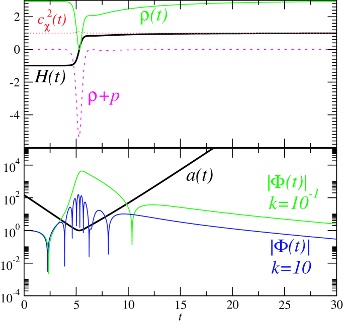
First, consider the fast bounce (FB) of Fig. 1. As shown in the upper panel, the universe starts in a quasi-de Sitter contracting phase, with and . It contracts with that initial rate up until , then it bounces at as the expansion rate grows very rapidly. It then reaches another quasi-de Sitter phase, albeit an expanding one. In our arbitrary time units, the bounce lasts about . Notice that at the density and the expansion rate become flat for an instant of time, meaning that at that point the equation of state reached the value – that is, the universe went through an instantaneous de Sitter point. Notice also that nothing special happens to the sound speed – indeed, in all our models the sound speed is well-behaved and is not crucial to any of our discussions.
The cosmological perturbations in the FB model are shown in the lower panel of Fig. 1, for two different wavelengths ( and ), along with the scale factor. As discussed above, we do not have a natural criterium to impose on the initial conditions of the Bardeen potential. Thus we chose, for all numerically evolved models below, to set and : then, getting anything else but a constant for asymptotically long times after the bounce would be evidence of mode mixing.
It can be seen that the newtonian potential is well-behaved at all times (as shown in the analytical solutions of the previous sections). For wavelengths longer than that of the mode the solutions for the perturbations are all identical, meaning that the bounce does not affect them differently. With our initial conditions all perturbations go through a sign change at around , which is just a manifestation of the relative growth of the dominant mode compared to an initially mixed-mode state.
Notice that the small-wavelength mode detaches from the behavior of the mode at around , which indicates that the small-wavelength mode almost reaches the oscillatory regime. Indeed, for wavelengths smaller than that of the mode the perturbations go through a period of oscillations which becomes longer as we consider smaller wavelengths. This means that these modes are small enough to be insensitive to the curvature radius created by the bounce. Equivalently, we can say that the modes experience a very small effective potential , so they simply oscillate.
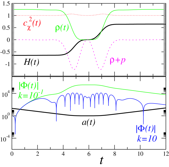
In Fig. 2 we show a bounce model (MB) in which the bounce itself happens over a longer period of time, . We have also set the parameters so that the instant of the bounce coincides with an instant when . Hence, in this model the bounce () is also a quasi-de Sitter point (); in other words, the background behaves, close to the bounce, like Minkowski spacetime. It is interesting, although not entirely unexpected, that even in this critical model the perturbations are entirely well behaved at all times.
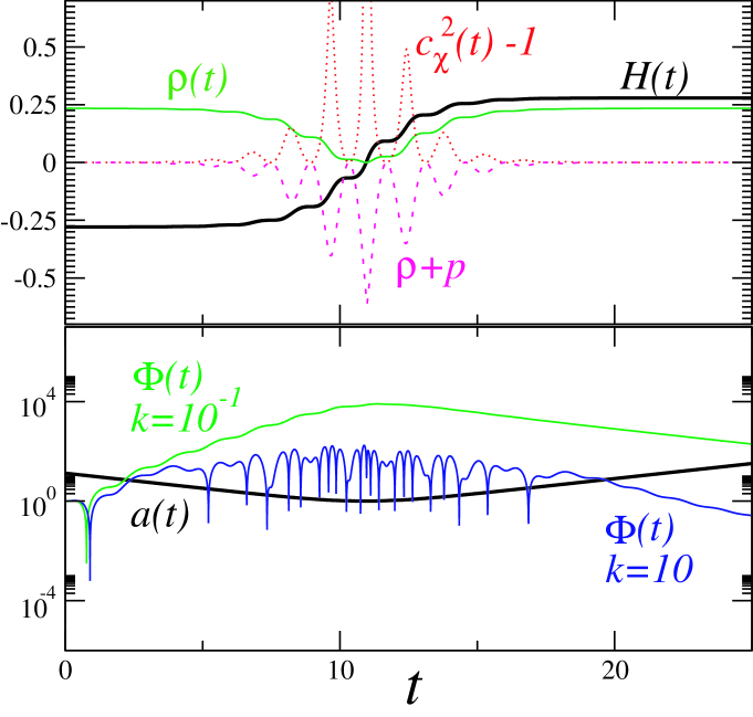
In Fig. 3 we show the SB model. Here the bounce is accompanied by many quasi-de Sitter instantaneous points (.) The bounce happens during a time scale of . The most telling characteristic of the perturbations is that now the mode with experiences more than 20 oscillations during the bounce, while in the MB model it only had time to perform about six oscillations.
The main result of this Section is that cosmological perturbations pass through the bounce with their spectrum essentially unchanged. However, our numerical evolution cannot address the important question whether there is mixing between the dominant and sub-dominant modes, before and after the bounce. This is due to the rapidly decaying nature of the sub-dominant solution after the bounce.
Let us consider the possibility of mode mixing by means of a simplified analytical model inspired by the numerically solved fast bounce scenario. Let us take the following model for the Hubble parameter:
| (43) |
which interpolates smoothly between a de Sitter phase with contraction rate and an expanding de Sitter phase with expansion rate . Notice that we have neglected the term , since the numerical analysis have shown that it only matters for perturbations of very small wavelength. Eq. (24) then becomes:
| (44) | |||
In order to get an analytical solution we assume that , and we take for simplicity. (Note that this is strictly equivalent to introducing a new variable and rescalling all the constants accordingly.) With these choices, the two linearly independent solutions to Eq. (24) are:
| (45) | |||||
| (46) |
where , , and and are the associated Legendre functions of the first and second kind, respectively [32].
Since we would like to connect this universe model with a previous contracting phase (before pre-cooling) and an ensuing expansion phase (after pre-heating), we should consider what happens with the two modes above both at early times () and at late time (). This is necessary if we give initial conditions for the perturbations and their time derivatives at some initial (early) time, and if we would like to follow their evolutions at late times and ask whether that choice of initial values implies a mixture of the two modes of Eqs. (45)-(46).
It turns out that the asymptotic limits () and () are very subtle for the associated Legendre functions: in fact, the limit is singular in the Legendre differential equation, which translates into the fact that the Legendre functions are almost degenerate – and, of course, without a complete basis of linearly independent functions we cannot accomodate an arbitrary set of initial condition. As a result, we need to expand the functions to 3rd order in the small parameters so as to break that degeneracy. The result is that, in the limit (), we get:
Here we have implicitly assumed that , so the series in non-integer powers of is ordered correctly.
Comparing the first two terms in Eqs. (5.4)-(5.4) one can see that they are identical, up to a constant. Only the third-order terms in these solutions have different factors. Therefore, if we want to assign arbitrary initial conditions to the perturbations at very early times, we need to go to third order in the series around . Since this small factor goes exponentially to zero as , this means that numerically it is very hard to select only one of the modes. Any choice of initial conditions that selected one mode at the expense of the other, if made at a very early time , would imply a fine-tuning of order . This means that quite generically, any natural choice of initial conditions at very early times will necessarily select a mixture of the two modes, and .
Consider now the limit ():
It can be noticed also in this limit that the two modes are degenerate up to second order in .
The conclusion we can draw from the solutions above at both asymptotic limits is that, in order to obtain a pure mode at one would need to fine-tune the initial conditions to order , and inspect the final solution up to the same order and precision. It should be evident that a numerical calculation would need an astonishing level of accuracy to be able to detect such minute differences. This explains why we could not address the question of mode mixing in the numerical analysis.
With these solutions at hand, one can ask the question: is it actually possible to avoid mixing when making a transition between two contracting or expanding de Sitter phases? We see on inspection of Eqs. (5.4) to (5.4), expanding the functions in time, that the general solution for the gravitational potential reads
| (51) |
where the coefficients , , and can be obtained formally from Eqs. (5.4) to (5.4). In the absence of mode mixing, one would expect the transition matrix relating to to be diagonal. As the coefficients of the modes are different from one side to the other, this is clearly not the case, so one expects mixing, at least in this simplified model.
As a result, if the contracting and expanding phases are of comparable durations, an initial condition in the contraction era which is a mixed state of the dominant and subdominant modes will become a very different mix of the dominant and subdominant modes at the end of the contraction era, in effect transferring power from one component to the other. This transfer can result in a large amplification of . This would mean that, provided there is a scale-invariant spectrum in before the bounce, however small its amplitude, and even if it is present only in the sub-dominant mode, the bounce can manage to amplify it to large values. However, this mechanism does not separate the spectrum from the amplitude, as, say, the curvaton models [33], because the curvature perturbation is, on large, cosmologically relevant scales, conserved through the bounce, and thus retains its amplitude as well as its spectral index.
6 Spectrum of perturbations in a K-bounce
There are two ways in which we can address the question about cosmological perturbations in K-bounce models. First, we could assume that there were no perturbations initially, and that a spectrum of cosmological perturbations was generated by the bounce itself, through the usual quantum mechanism. Second, we could equally well assume that the bounce only distorts a pre-existing spectrum of cosmological perturbations. Of course, in general both processes will occur, but in linear theory they can be treated separately and the final spectrum will be a combination of the two spectra. Let us briefly discuss the first possibility of producing the perturbations at the bounce itself.
While tempting to produce perturbations close to the bounce, one immediately faces a major difficulty, namely that it seems rather unlikely that natural, vacuum-like, initial conditions could be imposed close to the bounce. Indeed, with the expansion (29), one has in (20), so that switching back to the time variable , we obtain
| (52) |
where we have set, for simplicity, to unity, since we have seen above (numerically) that this quantity is completely regular through the bounce and actually hardly varies at all. To leading order in , Eq. (20) becomes
| (53) |
whose general solution is expressible in terms of hypergeometric functions. For all but the smallest wavelength modes, these happen to have no oscillatory part to which one could connect the vacuum initial condition . The evolution through the bounce itself is therefore completely arbitrary for all scales of cosmological interest. Hence, in what follows we shall be concerned exclusively with the second possibility, namely, of modifying a spectrum originally produced during the contracting phase prior to the bounce.
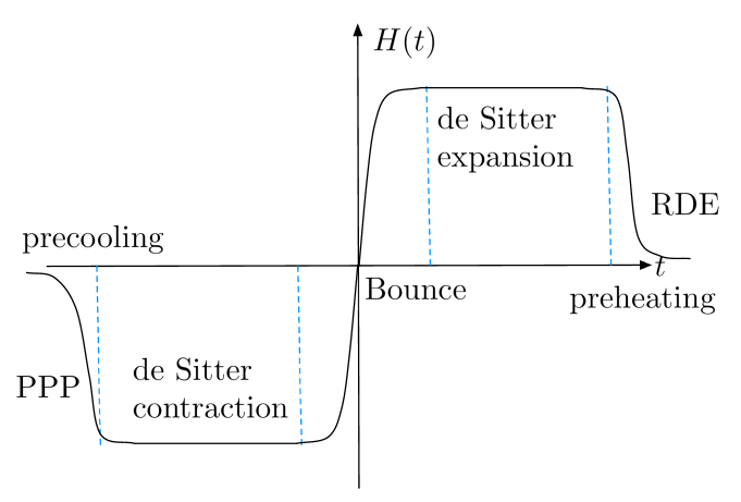
Recently, [15] considered a K-essence model in which the contracting phase prior to the bounce was described by near the bounce, which leads to . However, that approximation clearly breaks down at the bounce. We will now assume, in the same fashion, that a contracting phase not described by our K-bounce model has already taken place, and that a radiation-dominated era starts shortly after the bounce. The situation is summarized on Fig. 4. We will simply assume that the curvature perturbations are transmitted in a non-singular way through these precooling and preheating phases – as happens in the usual mechanism of preheating. Therefore, here we are just interested in the way an initial spectrum created in a pre-bounce era (before precooling) is affected by the bounce, and how that spectrum is transmitted to the radiation-dominated era after preheating. Given that all modes of interest are in the infrared limit (long wavelengths) before and after the bounce, we only need to ask what spectral distortions (if any) are introduced by the bounce.
The overall conclusion we can draw from the last section is that an initial spectrum of long-wavelength modes is entirely unaffected by the bounce: the long-wavelength modes all behave in exactly the same way, so their relative amplitudes remain unchanged. The curvature perturbation is conserved across the bounce for large enough wavelengths. What emerges from the numerical analysis discussed in the previous section is that for long, i.e. cosmologically relevant, wavelengths, the spectrum produced before the bounce, during the contracting phase, is essentially unchanged apart from an overall amplification factor for which, however, still leaves the curvature perturbation constant. Let us consider for instance the case of Fig. 2, very close to the bounce, and suppose the contracting phase lasted much longer in the past than indicated. Since we are working with arbitrary units in time, we are free to assume that the preheating-like phase begins, in this model, around , i.e. very shortly after the bounce. Note that we must assume that the expanding era is sufficiently close to the bounce in order to ensure a natural solution to the flatness problem.
Connecting the bounce with the radiation-dominated phase, in a way yet to elucidate, very shortly after this bounce took place, we end up with a spectrum of perturbations which is undistorted. (recall that our initial conditions were such that and .) In other words, the transfer matrix [12], i.e. the matrix that relates the initial amplitudes of the growing and decaying modes to their final amplitudes at some fiducial instant of time, does not depend on scale. As we have evolved the perturbations numerically, it is extremely difficult to extract information about the decaying mode. Instead, we focus on the spectrum of the perturbations at some point after the bounce has occurred.
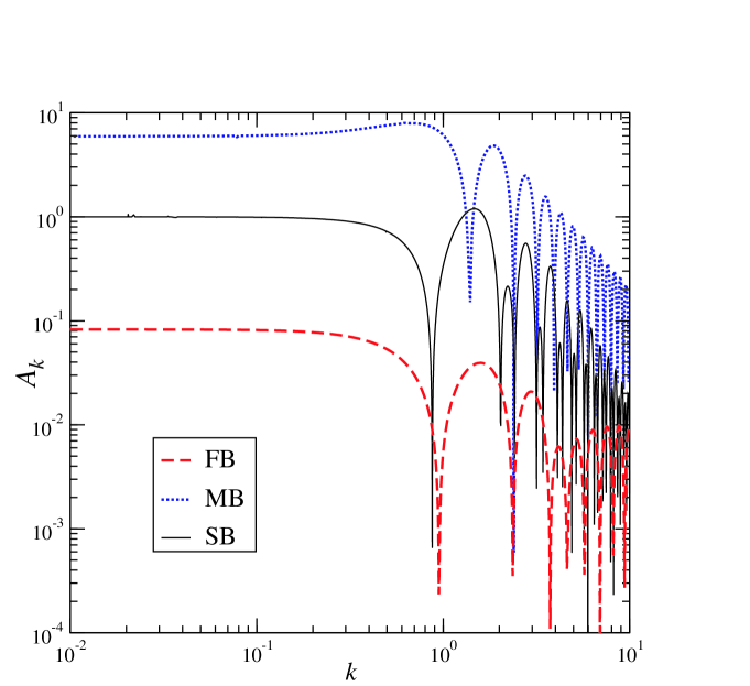
There are two ways in which we can compute the spectrum. First, we can use the dominant solution of Eq. (26), and calculate its amplitude as a function of the wavenumber . By setting all modes to the same initial value, we thus obtain the spectral distortions caused by the bounce. This is shown in Fig. 5 for the concrete models we considered. The main result is that for long-wavelengths (small ) the amplitudes are completely flat, meaning that the bounce does not distort the initial spectra. Notice also that, for the small wavelengths, the onset of the oscillatory regime influences their relative amplitudes, and the change in their spectrum seems to be model-dependent. In general, slow bounces seem to produce a decay in the spectrum for small wavelengths, whereas fast bounces have little to no overall effect over the UV sector of the spectrum apart from some oscillations.
The second method is to evaluate the amplitude of the long-wavelength modes after the bounce. This is useful in order to compute the amplification factor – which is only meaningful for those long wavelengths. We have obtained, for the three models we studied, , and for the FB, MB and SB models respectively – see Figs. 1-3. Note that these values are very much dependent on the initial time we put the initial conditions on. This means that in practice, much larger amplifications could easily be achieved. However, notice that the physically relevant function is the curvature perturbation . We have found, in agreement with [13], that in fact remains essentially constant – even if can be vastly amplified. This means that the physical observables are unaffected by the bounce.
7 Discussions and conclusions
Bouncing models have been proposed as possible alternatives to inflation. Even though such models seem to be able to solve at least some cosmological puzzles such as the horizon and flatness problems, many of them still face a basic difficulty of producing an almost scale-invariant spectrum of perturbation. The main reason for this failure is that there is no generally agreed upon way of making a bounce. In particular, this stems from the fact that General Relativity forbids a bounce to take place without spatial curvature or violations of the energy conditions.
Bouncing models have been built based either on a positive spatial curvature [12, 13] or many fluids [10] – one of them having negative energy. The results that have been obtained up to now are very strongly model-dependent, ranging from no effect whatsoever (the modes passing unaltered through the bounce), to a complete modification of the spectrum involving mode mixing. It has been argued that both the mode mixing and/or the spectral modifications could be due to either the spatial curvature and/or the presence of many degrees of freedom, and hence of entropy perturbations. Therefore, there has been no agreement about whether bounces would lead inevitably to spectral distortions. Hence the need to try and find a simple bouncing model with only one degree of freedom and no spatial curvature in the framework of GR.
We have achieved the construction of one degree of freedom simple bouncing models by means of a generalized scalar field theory. Our models violate most energy conditions, but still we have . However, because the phantom barrier () cannot be bypassed without some sort of singularity, such models cannot be very realistic, and must be embedded into a more complete theory containing at least the usual expanding radiation-dominated era. As we have shown, all our cosmological models flow to asymptotic de Sitter solutions with . This implies that the connection with the radiation era must be realized through some sort of preheating mechanism. Similarly, the contracting de Sitter solution is a repulsor from which all contracting solutions flow. This means that, going backwards in time, all pre-bounce solutions must have initiated from a contracting de Sitter stage. Again, in order to relate the bounce to a contracting universe dominated by a regular fluid such as dust or radiation, one must have a mechanism similar to preheating, but going the other way around, that we have called precooling – see Fig. 4.
We have found that, in these simple models, the propagation of perturbations is highly non-trivial: although the transition matrix which relates the growing and decaying modes before and after the bounce is wavelength-independent (no mode mixing in the terminology of the first of Refs. [12]), it is however non diagonal, so there is in general some amount of mixing between the two modes. Analytical calculations show that even an exponentially small initial contribution of the sub-dominant mode can lead to a high degree of mode mixing in the final spectrum of perturbations. Hence, if the two modes have different spectral tilts in the contraction era, the resulting spectrum will almost surely consist of a superposition of the two spectra.
We have also found that this mixing can lead to an amplification of the metric perturbations : any initial suppression of the sub-dominant mode deep in the contraction era would be offset by an equal amount of growth prior to the bounce, leading to potentially large amplification factors for . However, this does not impact the physically relevant curvature perturbation , which remains essentially constant despite the growth of , implying that the bounce does not affect physical observables.
8 Acknowledgments
R.A. would like to thank the Institut d’Astrophysique de Paris, and P.P., the Instituto de Física (Universidade de São Paulo), for their warm hospitality. We very gratefully acknowledge various enlightening conversations with Jérôme Martin, Nelson Pinto-Neto and Fabio Finelli. R.A. would like to thank João C. A. Barata for key comments on the theory of confluent hypergeometric functions. We also would like to thank CNPq, CAPES and FAPESP (Brazil), as well as COFECUB (France), for financial support.
References
References
- [1] D. N. Spergel et al, Ap. J. Suppl. 148, 175 (2003); D. N. Spergel et al, astro-ph/0603449, Ap. J. (2006).
- [2] A. Guth, Phys. Rev. D23, 347 (1981); A. Linde, Phys. Lett. B 108,389 (1982); A. Albrecht and P. J. Steinhardt, Phys. Rev. Lett 48, 1220 (1982); A. Linde, Phys. Lett. B 129, 177 (1983); A. A. Starobinsky, Pis’ma Zh. Eksp. Teor. Fiz. 30, 719 (1979) [JETP Lett. 30, 682 (1979)]; V. Mukhanov and G. Chibisov, JETP Lett. 33, 532 (1981); S. Hawking, Phys. Lett. B 115, 295 (1982); A. A. Starobinsky, Phys. Lett. B 117, 175 (1982); J. M. Bardeen, P. J. Steinhardt, and M. S. Turner, Phys. Rev. D28, 679 (1983); A. Guth, S. Y. Pi, Phys. Rev. Lett 49, 1110 (1982).
- [3] V. Mukhanov, “Inflationary cosmological perturbations”, talk given at the 22nd IAP colloquium, Inflation +25, Paris (2006).
- [4] G. Murphy, Phys. Rev. D8, 4231 (1973); A. A. Starobinsky, Sov. Astron. Lett. 4, 82 (1978); M. Novello and J. M. Salim, Phys. Rev. D20, 377 (1979); V. Melnikov and S. Orlov, Phys. Lett A70, 263 (1979); V.A. De Lorenci, R. Klippert, M. Novello and J.M. Salim, Phys. Rev. D65, 063501 (2002); J. C. Fabris, R. G. Furtado, P. Peter and N. Pinto-Neto Phys. Rev. D67 124003 (2003).
- [5] G. Veneziano, Phys. Lett. B 265, 287 (1991); M. Gasperini and G. Veneziano, Astropart. Phys. 1, 317 (1993); See also J. E. Lidsey, D. Wands, and E. J. Copeland, Phys. Rep. 337, 343 (2000) and G. Veneziano, in The primordial Universe, Les Houches, session LXXI, edited by P. Binétruy et al., (EDP Science & Springer, Paris, 2000).
- [6] J. Khoury, B. A. Ovrut, P. J. Steinhardt, and N. Turok, Phys. Rev. D64, 123522 (2001); hep-th/0105212; R. Y. Donagi, J. Khoury, B. A. Ovrut, P. J. Steinhardt, and N. Turok, JHEP 0111, 041 (2001).
- [7] C. Cartier, Scalar perturbations in an -regularised cosmological bounce, hep-th/0401036 (2004); M. Gasperini, M. Giovannini, G. Veneziano, Phys. Lett. B569, 113 (2003); Nucl. Phys. B694, 206 (2004).
- [8] R. Kallosh, L. Kofman, and A. Linde, Phys. Rev. D64 123523 (2001); J. Martin, P. Peter, N. Pinto-Neto, and D. J. Schwarz, Phys. Rev. D65, 123513 (2002) and references therein.
- [9] P. Peter, E. Pinho and N. Pinto-Neto, Phys. Rev. D75 023516 (2007).
- [10] P. Peter and N. Pinto-Neto, Phys. Rev. D65, 023513 (2002); P. Peter and N. Pinto-Neto, Phys. Rev. D66, 063509 (2002); F. Finelli, JCAP 0310, 011 (2003); P. Peter, N. Pinto-Neto and D. A. Gonzalez, JCAP 0312, 003 (2003).
- [11] V. Bozza and G. Veneziano, JCAP 0509, 007 (2005); Phys. Lett. B625, 177 (2005).
- [12] J. Martin and P. Peter, Phys. Rev. D68, 103517 (2003); C. Gordon and N. Turok, Phys. Rev. D67, 123508 (2003); J. Martin and P. Peter, Phys. Rev. Lett 92, 061301 (2004); Phys. Rev. D69, 107301 (2004).
- [13] L. E. Allen and D. Wands, Phys. Rev. D70, 063515 (2004).
- [14] R. H. Brandenberger and J. H. Traschen, Phys. Rev. D42: 2491-2504 (1990); L. Kofman, A. Linde and A. Starobinsky, Phys. Rev. Lett. 73: 3195-3198 (1994); Phys. Rev. D56: 3258-3295 (1997).
- [15] P. Creminelli and L. Senatore, hep-th/0702165.
- [16] N. Arkani-Hamed, H. C. Cheng, M. A. Luty and S. Mukohyama, JHEP 0405: 074 (2004), hep-th/0312099.
- [17] A. Sen, JHEP 0204: 048 (2002); ibid. 0207: 065 (2002); A. Sen, Mod. Phys. Lett. A17: 1797-1804 (2002).
- [18] E. Silverstein and D. Tong, Phys. Rev. D70: 103505 (2004).
- [19] M. Fairbairn and M. H. G. Tytgat Phys. Lett. B546: 1 (2002).
- [20] D. Wands, Phys. Rev. D60, 023507 (1999); F. Finelli and R. Brandenberger, Phys. Rev. D65, 103522 (2002).
- [21] L. R. Abramo and N. Pinto-Neto, Phys. Rev. D73: 063522 (2006).
- [22] M. Ostrogradski, Mem. Ac. St. Petersbourg VI, 4: 385 (1850).
- [23] V. I. Arnold, “Analytical Mechanics” (Springer, 1997).
- [24] R. P. Woodard, Avoiding Dark Energy with Modifications of Gravity, astro-ph/0601672 (2006).
- [25] V. F. Mukhanov, H. A. Feldman, and R. H. Brandenberger, Phys. Rep. 215, 203 (1992).
- [26] J. Garriga and V. F. Mukhanov, Phys. Lett. B 458, 219 (1999).
- [27] T. Chiba, T. Okabe and M. Yamaguchi, Phys. Rev. D 62, 023511 (2000); C. Armendariz-Picon, V. F. Mukhanov and P. J. Steinhardt, Phys. Rev. Lett. 85, 4438 (2000).
- [28] J.-P. Bruneton, On causality and superluminal behavior in classical field theories, gr-qc/0607055, (2006).
- [29] A. Vikman, Phys. Rev. D71: 023515 (2005); W. Hu, Phys. Rev. D71: 047301 (2005); R. Caldwell and M. Doran, arXiv: astro-ph/0501104; G.-B. Zhao, J.-Q. Xia, M. Li, B. Feng and X. Zhang, arXiv: astro-ph/0507482.
- [30] R. Brandenberger and F. Finelli, JHEP 0111: 056 (2001); R. Brandenberger, F. Finelli and S. Tsujikawa, Phys. Rev. D66: 083513 (2002).
- [31] L. J. Slater, “Confluent Hypergeometric Function” (Cambridge University Press, 1960).
- [32] M. Abramowitz and I. A. Stegun, “Handbook of mathematical functions” (Dover, 1972).
- [33] D. H. Lyth, C. Ungarelli and D. Wands, Phys. Rev. D67: 023503 (2003).