Cosmological Constraints on Isocurvature and Tensor Perturbations

Masahiro Kawasaki and Toyokazu Sekiguchi

Institute for Cosmic Ray Research, University of Tokyo
Kashiwa 277-8582, Japan,

We investigate cosmological constraints on primordial isocurvature and tensor perturbations, using recent observations of the cosmic microwave background and the large scale structure. We find that present observations are consistent with purely adiabatic initial conditions for the structure formation under any priors on correlations of isocurvature modes, and upper limits on the contribution of isocurvature and tensor perturbations are presented. We also apply the obtained constraints to some specific theoretical models, axion isocurvature perturbation models and curvaton models, and give some implications for theoretical models.

1 Introduction

Recent cosmological observations, such as the cosmic microwave background (CMB) and the large scale structure (LSS) provide us information on primordial perturbations which seed the structure of the present universe. All observations suggest that the primordial fluctuation is almost adiabatic and scale-invariant [1, 2]. Inflation is the most promising mechanism to generate the scale-invariant adiabatic fluctuation in the early universe. On the other hand, primordial isocurvature perturbations are also generally generated, along with the tensor perturbations, in the inflation universe. Many possible sources and mechanisms generating isocurvature perturbations are known such as axion, curvaton scenarios [3, 4] and multi-field inflation models.

Therefore it is expected that constraints on primordial isocurvature and tensor perturbations give us some useful information to build realistic inflation models and models in particle physics. Thus, constraints on primordial isocurvature perturbations have been investigated by many authors [5, 6, 7, 8, 9, 10, 11, 12] (For recent constraints we refer to [13, 14, 15]). However, there have been few investigations on cosmological models with both isocurvature and tensor perturbations. This is partly because in most inflation models tensor perturbations are expected to be small when (especially correlated) isocurvature perturbations are generated. However still some models predicts generation of both isocurvature and tensor perturbations [16, 17]. From phenomenological point of view, it is worth checking whether cosmological observations are consistent with purely adiabatic initial conditions even if we consider both isocurvature and tensor perturbations.

In this paper we investigate constraints on cosmological models with both isocurvature and tensor perturbations in light of cosmological observations of CMB and LSS. We use data from two recent cosmological observations, CMB temperature and polarization power spectra from WMAP 3-year result (WMAP3) and galaxy power spectrum from SDSS data release 4 of luminous red galaxy sample (SDSS DR4 LRG). We only consider models with one isocurvature mode along with adiabatic and tensor modes, which are simple but suggestive for various models predicting generation of isocurvature and tensor modes. We investigate the isocurvature mode by using three different priors on correlation between isocurvature and adiabatic modes; 1) uncorrelated, 2) totally correlated and 3) generally correlated models. The reason why we investigate uncorrelated and totally correlated models separately is that there are some simple models predicting definite correlations. For examples, the axion isocurvature perturbation model produces uncorrelated isocurvature mode and the totally correlated one is predicted in curvaton scenarios.

The structure of the paper is as follows. In Section 2 we briefly review the general initial perturbations of the structure formation which includes the isocurvature and tensor perturbations and we also gives the parametrization used to constrain the isocurvature perturbations there. In section 3 we give some examples of models with both isocurvature and tensor perturbations which are based on inflation scenarios. In section 4 we show the method to obtain the constraints on the isocurvature and tensor perturbations from the combined set of cosmological observations. In section 5 we present constraints on isocurvature and tensor perturbations from CMB and LSS. In section 6 we apply the obtained constraints on the isocurvature perturbation to some specific models; axion isocurvature perturbation models and curvaton scenarios. Section 7 is dedicated to conclusions and discussions.

2 Initial perturbations for the structure formation

Scalar perturbations are generally decomposed into five modes [18]; adiabatic mode (AD), CDM isocurvature mode (CI), baryon isocurvature mode (BI), neutrino isocurvature density mode (NID) and neutrino isocurvature velocity mode (NIV). In the framework of the linear perturbation theory, each mode evolves independently and observables in present universe such as the CMB angular power spectrum and the matter power spectrum are predicted by initial amplitude of each mode and their correlation.

In this paper we adopt the definition of initial perturbations for the structure formation in [18]. We use $X_{I}(\mathbf{k})$ for representing the initial perturbation of each mode.

$$X_{I}(\mathbf{k})=\left\{\begin{array}[]{ll}\zeta&(\mbox{for AD})\\ \mathcal{S}_{\mathrm{CDM}}&(\mbox{for CI})\\ \mathcal{S}_{b}&(\mbox{for BI})\\ \frac{3}{4(1-f_{\nu})}\mathcal{S}_{\nu}&(\mbox{for NID})\\ \frac{1}{1-f_{\nu}}\mathcal{V}_{\nu}&(\mbox{for NIV})\end{array}\right.$$ (2.6)

The right hand side of Eq. (2.6) is evaluated at the beginning of the structure formation. $\zeta$ is the gauge invariant curvature perturbation and $\mathcal{S}_{\mathrm{CDM}}$, $\mathcal{S}_{\mathrm{b}}$ and $\mathcal{S}_{\mathrm{\nu}}$ are the entropy perturbations of CDM, baryon and neutrino, separately. $\mathcal{V}_{\nu}=V_{\nu}-V_{\gamma}$ is the relative velocity perturbation of neutrino to photon. $f_{\nu}$ is the fraction of the neutrino species in the energy density of the radiations. For more detailed definition of each isocurvature mode, we refer to [18].

When we investigate observational constraints on various isocurvature modes in section 5, we consider only CI, NID and NIV modes. This is because the contribution of CDM and baryon isocurvature perturbations are brought together into isocurvature perturbations of matter

$$\mathcal{S}_{m}=\frac{\Omega_{\mathrm{CDM}}}{\Omega_{m}}\mathcal{S}_{\mathrm{CDM}}+\frac{\Omega_{b}}{\Omega_{m}}\mathcal{S}_{b}.$$ (2.7)

Thus, the constraint on $\mathcal{S}_{b}$ is easily obtained from that on $\mathcal{S}_{\mathrm{CDM}}$.

The auto and cross power spectra $\mathcal{P}_{ab}(k)$ of primordial perturbations can be written as

$$\mathcal{P}_{IJ}(k)\delta_{\mathbf{k}\mathbf{k}^{\prime}}=\frac{k^{3}}{2\pi^{2}}\langle X_{I}(\mathbf{k})^{*}X_{J}(\mathbf{k}^{\prime})\rangle.$$ (2.8)

Here subscripts $I$ and $J$ represent the adiabatic (AD) and four isocurvature modes (CI, BI, NID and NIV). We assume power spectra can be approximated as power-law:

$$\mathcal{P}_{IJ}(k)=A_{IJ}\left(\frac{k}{k_{0}}\right)^{n_{IJ}-1},$$ (2.9)

where $k_{0}$ is a pivot scale and we consistently take $k=0.05$ Mpc^-1 in the rest of this paper.

Throughout this paper we consider models with only one isocurvature mode besides adiabatic and tensor modes. This simplification enables us to capture what models are plausible to generate the initial fluctuations in the universe including isocurvature and tensor modes and the resultant constraints on isocurvature and tensor perturbations can be applied to many theoretical models based on inflation scenarios and particle physics. Since we have known that the primordial perturbations mainly consist of adiabatic perturbations, it is convenient to normalize the amplitudes of power spectra by the amplitude of the auto power spectrum of the adiabatic mode, $A_{\mathrm{AD}}$. Thus, we parametrize initial power spectra for the scalar perturbations as

$$A_{IJ}=A_{\mathrm{AD}}\left(\begin{array}[]{cc}1&B_{a}\cos\theta_{a}\\ B_{a}\cos\theta_{a}&B_{a}^{2}\end{array}\right),$$ (2.10)

where

$$B_{a} \equiv \sqrt{A_{aa}/A_{\mathrm{AD}}},$$ (2.11)

$$\cos\theta_{a} = A_{\mathrm{AD},a}/\sqrt{A_{aa}A_{\mathrm{AD}}}.$$ (2.12)

Subscripts $a$ represent some isocurvature mode being considered (CI, NID or NIV).

The tensor perturbations are also generated in inflation models. When we refer to tensor to scalar ratio $r$, we usually consider cases that the scalar perturbation is purely adiabatic. Since we are considering isocurvature perturbations along with the adiabatic perturbation here, we redefine $r$ as ’tensor to adiabatic ratio’. The power spectrum of tensor perturbations $\mathcal{P}_{g}(k)$ is written as follows:

$$\mathcal{P}_{g}(k) = A_{g}\left(\frac{k}{k_{0}}\right)^{n_{g}},$$ (2.13)

$$= rA_{\mathrm{AD}}\left(\frac{k}{k_{0}}\right)^{n_{g}},$$ (2.14)

where $n_{g}$ is the spectral index of the tensor perturbation.

Since each mode evolves independently within the framework of the linear perturbation theory, we can decompose perturbations of the fluids by initial modes. As for CMB, the brightness function of photon $\Theta_{l}$ is written as

$$\Theta_{l}(\mathbf{k},\eta)=\sum_{I}\Theta^{I}_{l}(\mathbf{k},\eta),$$ (2.15)

where $\Theta^{I}_{l}$ are brightness functions which evolve from different initial perturbation modes. We introduce a transfer function of photon for each mode $T^{I}_{l}(k,\eta)$:

$$\Theta^{I}_{l}(\mathbf{k},\eta)=T^{I}_{l}(k,\eta)X_{I}(\mathbf{k}).$$ (2.16)

Then we obtain the angular power spectra of CMB $C_{l}$,

$$C_{l} = \sum_{I,J}C_{l}^{IJ},$$ (2.17)

$$= A_{AD}\left[\hat{C}^{\mathrm{adi}}_{l}+2B_{a}\cos\theta_{a}\hat{C}^{\mathrm{cor}}_{l}+B_{a}^{2}\hat{C}^{\mathrm{iso}}_{l}+r\hat{C}^{\mathrm{tens}}_{l}\right]$$ (2.18)

where $\hat{C}_{l}$’s are the angular power spectra in cases that the amplitudes of the initial perturbations $A_{IJ}$ are set to be unity and subscripts $adi$, $iso$, $cor$ and $tens$ represent adiabatic auto, isocurvature auto, adiabatic-isocurvature cross and tensor power spectra, respectively. $\hat{C}_{l}$’s are given by

$$\hat{C}_{l}^{\mathrm{adi}} = \frac{4\pi}{2l+1}\int\frac{dk}{k}\left(\frac{k}{k_{0}}\right)^{n_{\mathrm{AD,AD}}-1}T^{\mathrm{AD}}_{l}(k)^{2},$$ (2.19)

$$\hat{C}_{l}^{\mathrm{iso}} = \frac{4\pi}{2l+1}\int\frac{dk}{k}\left(\frac{k}{k_{0}}\right)^{n_{a,a}-1}T^{a}_{l}(k)^{2},$$ (2.20)

$$\hat{C}_{l}^{\mathrm{cor}} = \frac{4\pi}{2l+1}\int\frac{dk}{k}\left(\frac{k}{k_{0}}\right)^{n_{\mathrm{AD},a}-1}T^{\mathrm{AD}}_{l}(k)T^{a}_{l}(k).$$ (2.21)

As for the matter power spectrum, $P(k)$ can be written in the same way,

$$P(k)=A_{AD}\left[\hat{P}^{\mathrm{adi}}(k)+2B_{a}\cos\theta_{a}\hat{P}^{\mathrm{cor}}(k)+B_{a}^{2}\hat{P}^{\mathrm{iso}}(k)\right],$$ (2.22)

where the hatted power spectra $\hat{P}(k)$’s are auto and cross power spectra with $A_{IJ}$ being unity.

3 Isocurvature perturbation based on inflation

So far we have considered generic models with isocurvature and tensor perturbations. In this section we consider a model with isocurvature and tensor perturbations based on inflation models. We assume there are two scalar perturbations generated during inflation. One is a curvature perturbation $\zeta_{*}$ and the other is a isocurvature perturbation $\mathcal{S}_{*}$. The curvature perturbation $\zeta_{*}$ raises only adiabatic mode at the beginning of structure formation, whereas the isocurvature perturbation $\mathcal{S}_{*}$ can generally produce both adiabatic and isocurvature perturbations at the beginning of the structure formation. Therefore we can write

$$\left(\begin{array}[]{c}\zeta\\ \mathcal{S}_{a}\end{array}\right)=\left(\begin{array}[]{cc}\mathcal{T}_{\zeta,\zeta_{*}}&\mathcal{T}_{\zeta,\mathcal{S}_{*}}\\ 0&\mathcal{T}_{\mathcal{S}_{a},\mathcal{S}_{*}}\end{array}\right)\left(\begin{array}[]{c}\zeta_{*}\\ \mathcal{S}_{*}\end{array}\right)$$ (3.23)

Here in the left hand side $\zeta$ and $\mathcal{S}_{a}$ are initial curvature and isocurvature perturbations for structure formation, separately. $\mathcal{T}$’s are transfer functions which represent how initial perturbations for structure formation are generated from perturbations during inflation. Since the curvature perturbation at over-horizon scale stays constant in the absence of isocurvature perturbations, $\mathcal{T}_{\zeta,\zeta_{*}}=1$. On the other hand $\mathcal{T}_{\zeta,\mathcal{S}_{*}}$ and $\mathcal{T}_{\mathcal{S}_{a},\mathcal{S}_{*}}$ depend on models. Then the initial power spectra for $\zeta$ and $\mathcal{S}_{a}$ are given by

$$\mathcal{P}_{\mathrm{AD,AD}}(k) = \mathcal{T}_{\zeta,\zeta_{*}}(k)^{2}\mathcal{P}_{\zeta_{*}}(k)+\mathcal{T}_{\zeta,\mathcal{S}_{*}}(k)^{2}\mathcal{P}_{\mathcal{S}_{*}}(k),$$ (3.24)

$$\mathcal{P}_{\mathrm{AD},a}(k) = \mathcal{T}_{\zeta,\mathcal{S}_{*}}(k)\mathcal{T}_{\mathcal{S}_{a},\mathcal{S}_{*}}(k)\mathcal{P}_{\mathcal{S}_{*}}(k),$$ (3.25)

$$\mathcal{P}_{a,a}(k) = \mathcal{T}_{\mathcal{S}_{a},\mathcal{S}_{*}}(k)^{2}\mathcal{P}_{\mathcal{S}_{*}}(k)$$ (3.26)

Generally $\zeta_{*}$ and $\mathcal{S}_{*}$ may be correlated, such in the case of multi-field inflation models [16, 17]. However, we assume that perturbations $\zeta_{*}$ and $\mathcal{S}_{*}$ are uncorrelated in this paper. Furthermore, we take power-law forms for the terms in the right hand sides of Eqs. (3.24)-(3.26) as

$$\mathcal{T}_{\zeta,\zeta_{*}}(k)^{2}\mathcal{P}_{\zeta_{*}}(k) = A_{\mathrm{adi1}}\left(\frac{k}{k_{0}}\right)^{n_{\mathrm{adi1}}-1},$$ (3.27)

$$\mathcal{T}_{\zeta,\mathcal{S}_{*}}(k)^{2}\mathcal{P}_{\mathcal{S}_{*}}(k) = A_{\mathrm{adi2}}\left(\frac{k}{k_{0}}\right)^{n_{\mathrm{adi2}}-1},$$ (3.28)

$$\mathcal{T}_{\zeta,\mathcal{S}_{*}}(k)\mathcal{T}_{\mathcal{S}_{a},\mathcal{S}_{*}}(k)\mathcal{P}_{\mathcal{S}_{*}}(k) = A_{\mathrm{cor}}\left(\frac{k}{k_{0}}\right)^{n_{\mathrm{cor}}-1},$$ (3.29)

$$\mathcal{T}_{\mathcal{S}_{a},\mathcal{S}_{*}}(k)^{2}\mathcal{P}_{\mathcal{S}_{*}}(k) = A_{\mathrm{iso}}\left(\frac{k}{k_{0}}\right)^{n_{\mathrm{iso}}-1},$$ (3.30)

where $A_{\mathrm{cor}}$ and $n_{\mathrm{cor}}$ are given by

$$A_{\mathrm{cor}} = \pm\sqrt{A_{\mathrm{adi2}}A_{\mathrm{iso}}},$$ (3.31)

$$n_{\mathrm{cor}} = \frac{n_{\mathrm{adi2}}+n_{\mathrm{iso}}}{2}.$$ (3.32)

Here the sign in the right hand side of the first line comes from a factor $\mathcal{T}_{\zeta,\mathcal{S}_{*}}\mathcal{T}_{\mathcal{S}_{a},\mathcal{S}_{*}}$ in Eq. (3.29), which can be either positive or negative. Furthermore, we use following parametrizations:

$$A_{\mathrm{AD}} = A_{\mathrm{adi1}}+A_{\mathrm{adi2}},$$ (3.33)

$$B_{a}^{2} = A_{\mathrm{iso}}/A_{\mathrm{AD}},$$ (3.34)

$$B_{a}\cos\theta_{a} = A_{\mathrm{cor}}/A_{\mathrm{AD}}.$$ (3.35)

Assuming single-field slow-roll inflation and $\mathcal{S}_{*}$ is the isocurvature perturbation for some scalar field ($\neq$ inflaton) whose mass is negligibly light compared with the Hubble parameter during inflation, the following inflation consistency relations should be satisfied:

$$n_{\mathrm{adi2}}-1=n_{g}=-\frac{A_{g}}{8A_{\mathrm{adi1}}}=-\frac{r}{8\sin^{2}\theta_{a}}.$$ (3.36)

We finally obtain the power spectra for CMB and matter,

$$C_{l} = A_{\mathrm{AD}}\left[\sin^{2}\theta_{a}\hat{C}_{l}^{\mathrm{adi1}}+\cos^{2}\theta_{a}\hat{C}_{l}^{\mathrm{adi2}}+B_{a}\cos\theta_{a}\hat{C}_{l}^{\mathrm{cor}}+B_{a}^{2}\hat{C}_{l}^{\mathrm{iso}}+r\hat{C}_{l}^{\mathrm{tens}}\right]$$ (3.37)

$$P(k) = A_{\mathrm{AD}}\left[\sin^{2}\theta_{a}\hat{P}_{l}^{\mathrm{adi1}}+\cos^{2}\theta_{a}\hat{P}_{l}^{\mathrm{adi2}}+B_{a}\cos\theta_{a}\hat{P}^{\mathrm{cor}}(k)+B_{a}^{2}\hat{P}^{\mathrm{iso}}(k)\right],$$ (3.38)

Note that there are two terms for adiabatic modes in each $C_{l}$ and $P(k)$. CMB and matter power spectra with subscript $adi1$ come from $\zeta_{*}$ and those with subscript $adi2$ come from $\mathcal{S}_{*}$.

4 Analysis method

We consider the flat $\Lambda$CDM model, and take the standard value 3.04 for massless neutrino species. We do not consider runnings in the spectral indices for scalar and tensor perturbations.

Since we are considering isocurvature and tensor perturbations, there exist six extra parameters $(B_{a},\ \cos\theta_{a},\ n_{\mathrm{AD},a},\ n_{a,a},\ r,\ n_{g})$ or $(B_{a},\ \cos\theta_{a},\ n_{\mathrm{adi2}},\ n_{\mathrm{iso}},\ r,\ n_{g})$ that are absent for a purely adiabatic case. However, for obtaining sensible constraints from the present cosmological observations, it is not suitable to treat all these parameters as free parameters. In this paper we adopt some simplifications and fix the spectral indices $(n_{\mathrm{AD},a},\ n_{a,a},n_{g})$ to some values. For the case considered in the previous section, we adopt the inflation consistency relation Eq. (3.36) to fix $(n_{\mathrm{adi2}},\ n_{\mathrm{iso}},\ n_{g})$. These simplifications reduce extra parameters to three primary free parameters $(B_{a},\ \cos\theta_{a},\ r)$.

Thus our models have the following nine primary parameters:

$$(\omega_{b},\omega_{\mathrm{CDM}},\theta_{\mathrm{sound}},\tau,A_{\mathrm{AD}},n_{adi},B_{a},\cos\theta_{a},r).$$ (4.39)

We investigate three models separately depending on the correlation of isocurvature modes; 1) uncorrelated, 2) totally correlated and 3) generally correlated isocurvature models. When we investigate uncorrelated $(\cos\theta_{a}=0)$ and totally correlated isocurvature $(\cos\theta_{a}=\pm 1)$ models, we fix $\cos\theta_{a}$ and when we investigate generally correlated isocurvature modes, we assign flat prior probabilities on the $\cos\theta_{a}$ in the range $[-1,1]$.

The likelihood of a model is assessed using the WMAP three-year (WMAP3) data and likelihood code [19, 20] and SDSS data release 4 luminous red galaxy sample (SDSS DR4 LRG) [2]. We include the nonlinear corrections for the matter power spectrum [21], and analytically marginalize over a bias parameter $b$ and a parameter for nonlinear correction $Q_{\mathrm{nl}}$. We modify the CAMB code [22] to generate CMB and matter power spectra. Likelihood surfaces are explored by Markov Chain Monte Carlo methods using CosmoMC [23]. We generate six chains for each model with isocurvature modes and their correlation and apply the Gelman and Rubin convergence test [24]. We finally obtain at least 150,000 samples for each model, and in some cases over 400,000 samples.

5 Constraints on isocurvature and tensor perturbations

5.1 Constraints on the uncorrelated isocurvature models

Firstly we investigate uncorrelated isocurvature models ($\cos\theta_{a}=0$). For the uncorrelated isocurvature models with tensor mode we impose inflation consistency relation

$$n_{g}=-r/8,$$ (5.40)

which is realized in a single-field slow-roll inflation model.

CI	NID	NIV

Figure 1: 1-dimensional likelihood distributions for uncorrelated isocurvature models with CI (left), NID (middle) and NIV (right) mode, respectively. In each panel we show the distributions for models without tensor modes using WMAP3 data only (red full), with tensor modes using WMAP3 data only (green dashed), without tensor modes using WMAP3 data combined with SDSS DR4 LRG data (blue dotted), with tensor modes using WMAP3 data combined with SDSS DR4 LRG data (magenta dot-dashed).

CI	NID	NIV

Figure 2: 68 % (full) and 95% (dashed) 2-dimensional constraints on the uncorrelated isocurvature models CI (left), NID (middle) and NIV (left) with tensor modes. We present constraints using WMAP3 data only (green) and combined with SDSS DR4 LRG data.

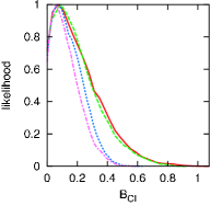
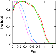
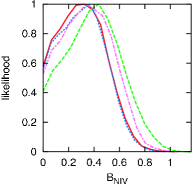
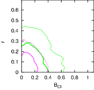
We present 1d-marginalized likelihood distributions for the uncorrelated isocurvature models in Figure 1. We also show 95% confidence limits (c.l.) on $B_{a}$ and $r$ for each models with (without) tensor modes from the combination of WMAP3 and SDSS DR4 LRG data in Table 1. The CDM isocurvature (CI) and neutrino isocurvature density (NID) modes are rather tightly constrained and there is no improvement in minimum $\chi^{2}$. On the other hand, presence of neutrino isocurvature velocity (NIV) modes tends to be favored by the present CMB and LSS data, though not yet at decisive level. Thus, we find no statistical support for finite contribution from uncorrelated isocurvature modes and CMB and LSS data are consistent with purely adiabatic initial scalar perturbations.

We also find 95% limits on tensor modes. Comparing with the constraint $r\leq 0.30$ (95% c.l.) for the model with purely adiabatic scalar perturbations [2], we find that the upper limits on $r$ for models with uncorrelated isocurvature are roughly same as that for the purely adiabatic model. This is because uncorrelated the isocurvature modes (except for uncorrelated NIV mode) and tensor mode contribute to the large scale anisotropy of CMB positively and there are no parameter degeneracy. For uncorrelated NIV mode, situations are little different since CMB power spectrum for NIV mode is relatively similar to that for AD mode [ see, e.g., Fig. 1. in [25]]. Thus, the upper limit on $r$ for uncorrelated NIV models is higher than those for other isocurvature models but it is still comparable with that for the purely adiabatic model.

	CI	NID	NIV
$B_{a}\leq$	0.31(0.33)	0.51(0.54)	0.69(0.62)
$r\leq$	0.26	0.25	0.31
$\Delta\chi^{2}_{\mathrm{min}}$	0(0)	0(0)	-1(-1)

Table 1: Constraints on $B_{a}$ and $r$ at 95% c.l. for uncorrelated isocurvature models with tensor modes (without tensor modes) from WMAP3+SDSS DR4 LRG. We also show the changes of the minimum $\chi^{2}$ values from the purely adiabatic model.

It is known there are some parameter degeneracies among fractions of isocurvature modes, $B_{a}$, and other cosmological parameters $\omega_{b}$, $\omega_{\mathrm{CDM}}$ and $n_{\mathrm{adi}}$. These degeneracies are understood by recognizing that the constraints on isocurvature modes rely mainly on the angular scale and the peak hight of the first acoustic peak in the CMB TT power spectrum. The relative hight of the first acoustic peak to the anisotropy at large angular scale, increases as the baryon density increases through compressions of the photon-baryon fluid. It also increases as the CDM density decreases and the early integrated Sachs-Wolfe effect is enhanced. Finally the peak height increases as the spectral index increases which leads to larger primordial fluctuations in small scales. For CI and NID modes, increase in $B_{a}$ decreases the relative peak hight of the acoustic peak. Thus some cancelations exist among $B_{a}$, $\omega_{b}$, $\omega_{\mathrm{CDM}}$ and $n_{s}$ and parameter degeneracies arise. But for NIV mode, increase in $B_{a}$ does not decrease the peak hight much and parameter degeneracies in NIV models are weaker than in uncorrelated CI and NID models. Though the peak hight has also strong dependence of the optical depth $\tau$, the polarization power spactra (TE and EE) of WMAP3 constrains $\tau$ tightly and no parameter degeneracy between $B_{a}$ and $\tau$ is seen. Some parameter degeneracies such as degeneracy between $B_{a}$ and $\omega_{\mathrm{CDM}}$ are broken by inclusion of LSS data and the constraints on $B_{a}$ improve (for CI and NID modes seen in Figure 1).

5.2 Constraints on totally correlated isocurvature models

Next we investigate totally correlated isocurvature models ($\cos\theta_{a}=\pm 1$). Firstly we define parameters for collecting both positively ($\cos\theta_{a}=1$) and negatively ($\cos\theta_{a}=-1$) correlated isocurvature models as

$$B_{a}^{\prime} = B_{a}\cos\theta_{a}=\left\{\begin{array}[]{cc}B_{a}&(\mbox{for }\cos\theta_{a}=1)\\ -B_{a}&(\mbox{for }\cos\theta_{a}=-1)\end{array}\right..$$ (5.43)

$B_{a}^{\prime}$ take either positive, 0 and negative values. For totally correlated isocurvature models with tensor modes we assume scale invariant tensor perturbations $n_{g}=1$.

CI	NID	NIV

Figure 3: 1-dimensional likelihood distributions for totally correlated isocurvature models . Considered isocurvature and tensor modes and combinations of data are same as Figure 3.

CI	NID	NIV

Figure 4: 68 % and 95% 2-dimensional constraints on the totally correlated isocurvature models with tensor modes. Contours are same as Figure 2.

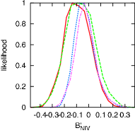
We show 1d-marginalized likelihood distributions for totally correlated isocurvature models in Figure 3. 95 % limits and relative changes in minimum $\chi^{2}$ from the purely adiabatic modes are presented in Table 2. We find no improvement in $\chi^{2}$ values and the present observations of CMB and LSS are consistent with the purely adiabatic initial conditions. For any isocurvature modes, the limits on $B_{a}$ for totally correlated models are found to be more stringent than for uncorrelated models. This is because, for totally correlated models, the correlation terms $\hat{C}_{l}^{\mathrm{cor}}$ and $\hat{P}^{\mathrm{cor}}(k)$ give significant contributions to the CMB and matter power spectra (see Eqs. (2.18) and (2.22)), which is not present for uncorrelated models. Therefore both CMB and matter power spectra are affected much if totally correlated isocurvature perturbations are present and limits becomes more stringent.

On the other hand the constraints on tensor modes $r$ for CI and NID modes becomes weaker, compared to those for uncorrelated models. This is because anti-correlated CI and NID modes decrease the anisotropies in large angular scales of the CMB TT power spectrum, which can be partly canceled by contributions from tensor modes. However, the constraints on tensor modes are not affected much for correlated NIV mode.

	CI	NID	NIV
$B^{\prime}_{a}$	$\leq$ 0.056(0.087)	$\leq$ 0.118(0.173)	$\leq$ 0.130(0.101)
	$\geq$ -0.129(-0.080)	$\geq$ -0.151(-0.090)	$\geq$ -0.189(-0.174)
$r\leq$	0.49	0.44	0.30
$\Delta\chi^{2}_{\mathrm{min}}$	0(0)	0(0)	0(0)

Table 2: Constraints for totally correlated models with tensor modes (without tensor modes) from WMAP3+SDSS DR4 LRG. We show $B^{\prime}_{a}$ and $r$ at 95 % c.l. and the changes of the minimum $\chi^{2}$ values from the purely adiabatic model.

5.3 Constraints on generally correlated isocurvature models

CI	NID	NIV

Figure 5: 1-dimensional likelihood distributions for generally correlated isocurvature models with CI (left), NID (middle) and NIV (right) mode. In each panel, we show distributions for models without tensor modes (red full), with tensor modes imposed inflation consistency relations (green dotted) and with tensor modes with fixed spectral index $n_{g}=1$ (blue dashed).

CI	NID	NIV

Figure 6: 68% (solid) and 95% (dashed) 2-dimensional constraints on the generally correlated isocurvature models. We present constraints for models with CI (left), NID (middle) and NIV (right) mode, separately. In each panel, we show constraints on models without tensor modes (red), with tensor modes imposed inflation consistency relations (green) and with tensor modes with fixed spectral index $n_{g}=1$ (blue). Black dashed lines represents $\cos\theta_{a}=\pm 1$.

CI	NID	NIV

Figure 7: 68 % and 95% 2-dimensional constraints on the totally correlated isocurvature models with tensor modes. Contours are same as Figure 6.

We finally investigate generally correlated isocurvature models ($-1\leq\cos\theta_{a}\leq 1$). For models with generally correlated isocurvature modes and tensor modes we consider two versions of models, models on which the inflation consistency relations Eq. (3.36) is imposed  and models with fixed spectral index $n_{g}=1$ for tensor modes.

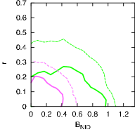
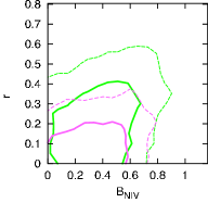
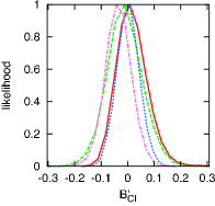
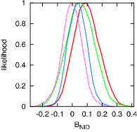
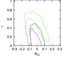
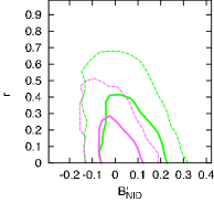
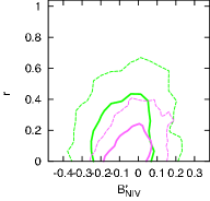
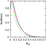
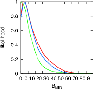
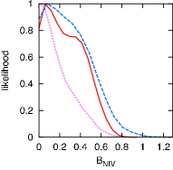
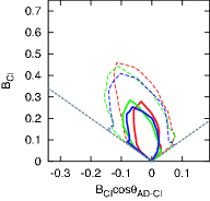
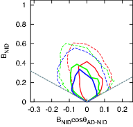
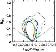
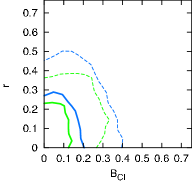
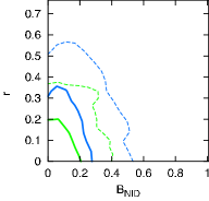
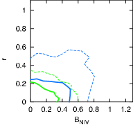
We present the 1d-marginalized likelihood distributions for generally correlated isocurvature models in Figure 5, and 2d likelihood contours in Figure 6. We also show 95% confidential limits for $B_{a}$ and $r$, mean values and 68% confidential limits for $\cos\theta_{a}$ and changes in minimum $\chi^{2}$ values from the purely adiabatic models in Table 3-5. Still, we find that observations are consistent with adiabatic initial conditions.

The upper bounds for $B_{a}$ are similar to the uncorrelated isocurvature models. These results are also guessed from the results obtained in Section 5.1 and 5.2, since, as we have seen, the allowed contribution of isocurvature perturbations are higher for uncorrelated isocurvature models than those for totally correlated modes.

We also present constraints for isocurvature and tensor perturbations in Figure 7. We can see that when we impose inflation consistency relations, upper bounds for tensor modes $r$ are roughly same as those for uncorrelated isocurvature models. This can be understood as follows. When correlations of isocurvature perturbations with adiabatic perturbations are either positively or negatively large ($\cos^{2}\theta_{a}\simeq 1$), the spectral index for tensor modes $n_{g}$ takes large negative values for fixed values for $r$, resulting in too much fluctuations for CMB anisotropy at large angular scales, which is disfavored from observations. Therefore large $r$ is allowed only when the correlation of isocurvature perturbations is small and hence the resulted bounds on $r$ are similar to those for uncorrelated isocurvature models. On the other hand, when we take the fixed spectral index for tensor modes, $n_{g}=1$, correlations of isocurvature perturbations can become large and the bounds for $r$ weaken as in the cases for totally correlated isocurvature and tensor perturbation models with $n_{g}=1$.

	CI	NID	NIV
$B_{a}\leq$	0.28	0.31	0.58
$\cos\theta_{a}$	$-0.25\pm 0.52$	$0.03\pm 0.62$	$0.05\pm 0.50$
$r\leq$	0.32	0.28	0.31
$\Delta\chi^{2}_{\mathrm{min}}$	0	0	-2

Table 3: Constraints for generally correlated models with tensor modes imposed inflation consistency relations on from WMAP3+SDSS DR4 LRG. We show 95% c.l. for $B_{a}$ and $r$, mean values and 68% c.l. for $\cos\theta_{a}$, and changes of the minimum $\chi^{2}$ values from the purely adiabatic model.

	CI	NID	NIV
$B_{a}\leq$	0.29	0.41	0.76
$\cos\theta_{a}$	$-0.04\pm 0.43$	$-0.10\pm 0.47$	$0.06\pm 0.34$
$r\leq$	0.43	0.50	0.73
$\Delta\chi^{2}_{\mathrm{min}}$	0	0	-2

Table 4: Same as Table 3 except for $n_{g}=1$.

	CI	NID	NIV
$B_{a}\leq$	0.33	0.47	0.59
$\cos\theta_{a}$	$-0.06\pm 0.34$	$0.06\pm 0.45$	$0.14\pm 0.40$
$\Delta\chi^{2}_{\mathrm{min}}$	0	0	-2

Table 5: Constraints for generally correlated models without tensor modes from WMAP3+SDSS DR4 LRG.

6 Application

In this section we apply the constraints on the isocurvature perturbation obtained in the previous section to some specific models of particle cosmology. We investigate two kinds of models, axion isocurvature perturbation models and curvaton scenarios.

6.1 Constraints on axion isocurvature perturbation and inflation models

Axion, which is originally proposed as a remedy for strong CP problem in QCD [26, 27, 28], is a candidate for CDM. The properties of axion, such as the decay constant and its couplings to ordinary matters are constrained from various observations of astrophysical and cosmological phenomena [29, 30]. In inflationary universe, the axion field has CDM isocurvature perturbations [31, 32, 33, 34, 35, 36, 37, 38] and they are constrained from observations of CMB and LSS [39, 40]. Firstly, we briefly review how the axion becomes CDM and its isocurvature fluctuation arises in the early universe.

We consider the case where the PQ symmetry is spontaneously broken when the universe is at the stage of inflation. During inflation the expectation value of the axion field is very smooth but fluctuates by the amount of the Hubble parameter $H_{\mathrm{inf}}$. The mean value of the axion $\chi$ and its fluctuation $\delta\chi$ can be represented as

$$\chi=f_{a}\theta_{i},$$ (6.44)

$$\delta\chi=H_{\mathrm{inf}}/2\pi.$$ (6.45)

Here, $f_{a}$ is the axion decay constant and $\theta_{i}$ is the initial phase of the axion field which takes an arbitrary value between $-\pi$ and $\pi$.

When the cosmic temperature is much higher than the QCD scale ($T\gg\Lambda_{\mathrm{QCD}}$), the axion has no potential and its field value stays constant. As the universe expands and its temperature decreases, the universe undergoes the QCD phase transition and the axion obtains mass which depends on the temperature $T$ as  [41]

$$m_{\chi}(T)=\lambda m_{\chi}(T\!=\!0)\left(\frac{T}{\Lambda_{\mathrm{QCD}}}\right)^{p},$$ (6.46)

where $\lambda\simeq 0.1$ and $p\simeq-4$. When the axion mass becomes equal to the Hubble parameter $[m_{\chi}(T)\sim H(T))$ ], the axion field starts to oscillate. After the axion starts oscillation its energy density scales as $a^{-3}$ and behaves as CDM. The density parameter of the axion is given by

$$\omega_{\chi}\equiv\Omega_{\chi}h^{2}=4.3\times\gamma~{}\theta_{i}^{2}\left(\frac{\Lambda_{\mathrm{QCD}}}{200\mbox{MeV}}\right)^{-2/3}\left(\frac{m_{\chi}(T\!=\!0)}{1\mu\mbox{eV}}\right)^{-7/6},$$ (6.47)

where $\gamma$ is the dilution factor. If there occurs no entropy release after the axion starts oscillation, $\gamma=1$. The mass of the axion at zero temperature is determined by its decay constant $f_{a}$ [42] as

$$m_{\chi}(T\!=\!0)=1.3\times 10^{-3}\mbox{eV}\left(\frac{f_{a}}{10^{10}\mbox{GeV}}\right)^{-1}.$$ (6.48)

Thus Eq. (6.47) can be rewritten in terms of $f_{a}$ as

$$\omega_{\chi}=1.0\times 10^{-3}\times\gamma\theta_{i}^{2}\left(\frac{\Lambda_{\mathrm{QCD}}}{200\mbox{MeV}}\right)^{-2/3}\left(\frac{f_{a}}{10^{10}\mbox{GeV}}\right)^{7/6}.$$ (6.49)

The axion isocurvature (entropy) perturbation is written as

$$\mathcal{S}_{\chi}\equiv\frac{\delta n_{\chi}}{n_{\chi}}-\frac{\delta n_{\gamma}}{n_{\gamma}},$$ (6.50)

where $n_{\chi}$ and $n_{\gamma}$ are the number densities of axion and photon, respectively. Axion isocurvature perturbation is given by the fluctuation of the axion field during inflation,

$$\mathcal{S}_{\chi}=2\frac{\delta\chi}{\chi}=\frac{H_{\mathrm{inf}}}{\pi f_{a}\theta_{i}},$$ (6.51)

where we have used Eqs. (6.44) and (6.45) at the second equality.

We consider the general case where CDM consists of axion and other particles and assume that only axion contributes to isocurvature perturbation. Then the CDM isocurvature perturbation are given by

$$\mathcal{S}_{\mathrm{CDM}}=\frac{\omega_{\chi}}{\omega_{\mathrm{CDM}}}\mathcal{S}_{\chi}.$$ (6.52)

The curvature perturbation $\zeta$ and tensor perturbations $h_{+,\times}$ are also generated during inflation and is written as

$$\zeta = -\frac{H_{\mathrm{inf}}}{d\phi/dt}\delta\phi,$$ (6.53)

$$h_{+,\times} = \frac{H_{\mathrm{inf}}}{\sqrt{2}M_{\mathrm{Pl}}},$$ (6.54)

where $\phi$ is the field value of the inflaton and $M_{\mathrm{Pl}}\equiv\sqrt{8\pi G}$ is the reduced Planck mass. We thus obtain power spectra of the adiabatic, CDM isocurvature and tensor modes as

$$A_{\mathrm{AD}} = \frac{H_{\mathrm{inf}}^{2}}{8\pi^{2}M_{\mathrm{Pl}}^{2}\epsilon},$$ (6.55)

$$A_{\mathrm{CI}} = \frac{\omega_{\chi}^{2}}{\omega_{\mathrm{CDM}}^{2}}\frac{H_{\mathrm{inf}}^{2}}{\pi^{2}f_{a}^{2}\theta_{i}^{2}},$$ (6.56)

$$A_{g} = \frac{H_{\mathrm{inf}}^{2}}{6\pi^{2}M_{\mathrm{Pl}}^{2}},$$ (6.57)

$$n_{\mathrm{AD}}-1 = -6\epsilon+2\eta,$$ (6.58)

$$n_{\mathrm{CI}}-1 = n_{g}=-2\epsilon.$$ (6.59)

Here we assume slow roll inflation and $\epsilon$ and $\eta$ are slow roll parameters given by

$$\epsilon = \frac{1}{2}M_{\mathrm{Pl}}^{2}\left(\frac{dV/d\phi}{V}\right)^{2},$$ (6.60)

$$\eta = M_{\mathrm{Pl}}^{2}\frac{d^{2}V/d\phi^{2}}{V}.$$ (6.61)

Since the axion isocurvature and the curvature perturbations are uncorrelated, $\cos\theta_{\mathrm{CI}}=0$. Using Eq. (2.11) with Eqs. (6.52), (6.55) and (6.56), we obtain $B_{\mathrm{CI}}$ and $r$ as

$$B_{\mathrm{CI}} = \frac{\omega_{\chi}}{\omega_{\mathrm{CDM}}}\frac{2\sqrt{2\epsilon}M_{\mathrm{Pl}}}{f_{a}\theta_{i}},$$ (6.62)

$$r = 16\epsilon.$$ (6.63)

Figure 8: Constraints on the axion decay constant and Hubble parameter in the inflation universe. The colored regions are excluded by cosmic density of the axion (red), SN1987A (blue) and axion isocurvature perturbation (green).

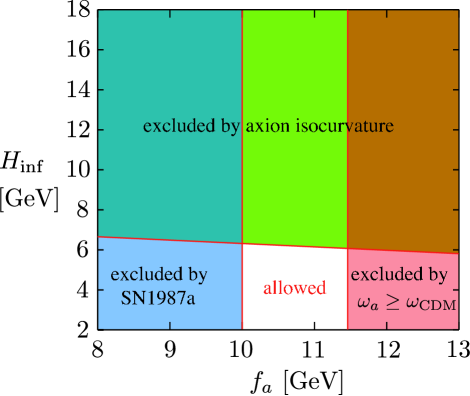
We are now ready to study constraints on axion and inflation models. From now on, we take $\Lambda_{\mathrm{QCD}}=200$ MeV, $\theta_{i}=1$ and assume no entropy release occurs after axion starts oscillation, i.e. $\gamma=1$. Firstly we obtain a upper bound on the axion decay constant $f_{a}$ from the requirement that the energy density of axion should not exceed the observed matter density in the present universe, $\omega_{\chi}\leq\omega_{\mathrm{CDM}}$. Combined with the lower bound obtained from supernovae 1987a [43] the axion decay constant should be in following range.

$$10^{10}\mbox{GeV}\leq f_{a}\leq 4.1\times 10^{11}\mbox{GeV}.$$ (6.64)

With using the bound for the CDM isocurvature mode in Table 1 we obtain the limits on the inflation parameters as

$$H_{\mathrm{inf}} \leq 10^{7}\mbox{GeV},$$ (6.65)

$$\epsilon \leq 10^{-16},$$ (6.66)

$$-0.05\leq \eta \leq 0.06.$$ (6.67)

We also present obtained bound in the $f_{a}$-$H_{\mathrm{inf}}$ plane in Figure 8. From Eqs. (6.55), (6.47) and (6.62) the ratio of the CDM isocurvature perturbation to the adiabatic one $B_{\mathrm{CI}}$ is written as

$$B_{\mathrm{CI}}=6.9\times 10^{-2}\left(\frac{\omega_{\mathrm{CDM}}}{0.1}\right)^{-1}\left(\frac{A_{\mathrm{AD}}}{2.1\times 10^{-9}}\right)^{1/2}\left(\frac{H_{\mathrm{inf}}}{10^{7}\mbox{GeV}}\right)\left(\frac{f_{a}}{10^{10}\mbox{GeV}}\right)^{1/6}\propto H_{\mathrm{inf}}f_{a}^{1/6}.$$ (6.68)

Therefore the upper bound on the Hubble parameter $H_{\mathrm{inf}}$ during inflation becomes lower as $f_{a}$ takes larger value.

The resultant constraints on $f_{a}$ and $H_{\mathrm{inf}}$ are comparable with those in [40], where the authors used the constraints on isocurvature and tensor modes derived by considering models with either of them, not both. We have analyzed models with both isocurvature and tensor modes but constraints on $H_{\mathrm{inf}}$ have not improved much. This is because the axion model predicts much less tensor perturbation than isocurvature one since $f_{a}\ll M_{\mathrm{Pl}}$. Thus, the obtained constraints on $f_{a}$ and $H_{\mathrm{inf}}$ do not change by inclusion of tensor modes. We can say oppositely that if nonzero contributions of tensor modes are suggested by future observations, the axion isocurvature model will be completely excluded.

In the case where the initial misalignment of axion field is accidentally much smaller than its natural value, $\theta_{i}\ll 1$, the constraints on the axion decay constant weakens since initial amplitude for the oscillation of axion field becomes smaller.

$$\omega_{\chi}\propto f_{a}^{7/6}\theta_{i}^{2}.\\$$ (6.69)

The constraints on $H_{\mathrm{inf}}$ also weakens. Although the amplitude of the isocurvature perturbation in axion field becomes larger by decrease of initial misalignment, however, its fraction in CDM isocurvature perturbation becomes smaller since the fractions of axion in CDM becomes lower.

$$B_{\mathrm{CI}}\propto f_{a}^{1/6}\theta_{i}H_{\mathrm{inf}}.$$ (6.70)

As we stated in the early part of this section, we have so far considered the case where the PQ symmetry is spontaneously broken during inflation. When the PQ symmetry is not broken during inflation or restored by the reheating after inflation, the inflation scale $H_{\mathrm{inf}}$ is not bounded by the constraints on the CDM isocurvature perturbations.

6.2 Constraints on curvaton models

In curvaton scenarios curvature perturbations are generated from the fluctuation of a scalar field ($=$ curvaton) which is isocurvature at the epoch of inflation. We firstly briefly review curvaton scenarios and then apply the constraints obtained in the previous section to them.

We represent a curvaton field as $\sigma$ and an inflaton field as $\phi$. Here we consider the case that the curvaton field is sufficiently light compared with the Hubble parameter during inflation. Then the mean value and fluctuation of the curvaton field are given as

$$\sigma = \sigma_{i},$$ (6.71)

$$\delta\sigma = \frac{H_{\mathrm{inf}}}{2\pi}$$ (6.72)

We represents the curvature perturbation generated during inflation as $\zeta_{*}$ and the isocurvature perturbation of the curvaton field as $\mathcal{S}_{\sigma}=2\delta\sigma/\sigma_{i}$.

Until the Hubble parameter of the universe becomes below the mass of the curvaton mass, the expectation value of the curvaton field is constant. After the Hubble parameter becomes comparable to the mass of the curvaton, the curvaton field starts oscillation and its energy dominates the universe. When the curvaton starts dominating the density of the universe, its fluctuation generates the curvature perturbation. After the curvaton decays, its energy turns into the radiation. If the curvaton produce the CDM, baryon or lepton number, their fluctuations also obey the fluctuation of the curvaton before its decay. Then various perturbations that are relevant for the structure formation are given by

$$\zeta = \zeta_{*}+\frac{1}{3}\mathcal{S}_{\sigma},$$ (6.73)

$$\mathcal{S}_{\mathrm{CDM}} = (r_{\mathrm{CDM}}-1)\mathcal{S}_{\sigma}+f_{\nu}\mathcal{S}_{\nu},$$ (6.74)

$$\mathcal{S}_{b} = (r_{\mathrm{B}}-1)\mathcal{S}_{\sigma}+f_{\nu}\mathcal{S}_{\nu},$$ (6.75)

$$\mathcal{S}_{\nu} = \frac{45}{7}\left(\frac{\xi}{\pi}\right)^{2}(r_{\mathrm{L}}-1)\mathcal{S}_{\sigma},$$ (6.76)

where $r_{\mathrm{CDM}}$, $r_{\mathrm{B}}$, $r_{\mathrm{L}}$ are the fractions of the CDM, baryon number and lepton number densities produced by or after the decay of the curvaton in the present densities. $\xi$ is the neutrino asymmetry parameter and we keep only the leading term of order in $\xi/\pi$ in Eq. (6.76) since $\xi$ is constrained from Big Bang Nucleosynthesis (BBN)[44] using the the observed helium abundance in [45] as

$$|\xi|\leq 0.07.$$ (6.77)

The neutrino isocurvature density perturbation $\mathcal{S}_{\nu}$ in Eq. (6.76) comes from the isocurvature perturbation in lepton number density $\mathcal{S}_{L}\equiv(\delta n_{\mathrm{L}}/n_{\mathrm{L}}-\delta n_{\gamma}/n_{\gamma})$ [47]. This is because nonzero lepton number density in the universe $n_{L}\neq 0$ affects the energy density of neutrino via changing the distribution function function of neutrino through nonzero chemical potential. The lepton number density and neutrino energy density are both written in terms of neutrino asymmetry parameter $\xi$ as

$$n_{L}=N_{\nu}\frac{\zeta(3)}{\pi^{2}}T_{\nu}^{3}\left[\frac{\xi}{\pi}+\left(\frac{\xi}{\pi}\right)^{3}\right],$$ (6.78)

$$\rho_{\nu}=N_{\nu}\frac{7\pi^{2}}{120}T_{\nu}^{4}\left[1+\frac{30}{7}\left(\frac{\xi}{\pi}\right)^{2}+\frac{15}{7}\left(\frac{\xi}{\pi}\right)^{4}\right].$$ (6.79)

Keeping only leading terms in $\xi/\pi$, we can relate the neutrino isocurvature perturbation $\mathcal{S}_{\nu}$ and the isocurvature perturbation for lepton number density $\mathcal{S}_{\mathrm{L}}$

$$\mathcal{S}_{\nu}=\frac{45}{7}\left(\frac{\xi}{\pi}\right)^{2}\mathcal{S}_{\mathrm{L}},$$ (6.80)

which yields Eq. (6.76).

More generally, the curvaton possibly decays before it completely dominates the universe. We therefore phenomenologically parametrize the various perturbations by using $r_{\mathrm{R}}\equiv\rho_{\sigma}/\rho_{T}$, the ratio of curvaton energy density just before its decay to the total energy density just after the curvaton decay, and then initial perturbations for the structure formation are written as

$$\zeta = \zeta_{*}+\frac{r_{\mathrm{R}}}{3}\mathcal{S}_{\sigma}$$ (6.81)

$$\mathcal{S}_{\mathrm{CDM}} = (r_{\mathrm{CDM}}-r_{\mathrm{R}})\mathcal{S}_{\sigma}+f_{\nu}\mathcal{S}_{\nu}$$ (6.82)

$$\mathcal{S}_{b} = (r_{\mathrm{B}}-r_{\mathrm{R}})\mathcal{S}_{\sigma}+f_{\nu}\mathcal{S}_{\nu}$$ (6.83)

$$\mathcal{S}_{\nu} = \frac{45}{7}\left(\frac{\xi}{\pi}\right)^{2}(r_{\mathrm{L}}-r_{\mathrm{R}})\mathcal{S}_{\sigma}.$$ (6.84)

In the case the curvaton decays after it completely dominates the universe and its energy turns into radiation nearly completely, $r_{\mathrm{R}}=1$.

Now we are prepared to obtain constraints on curvaton scenarios. For simplicity, we consider the case that the curvature perturbation generated at the inflation epoch is negligible ($\zeta_{*}=0$) and the curvature perturbation is created by the curvaton. In that case the isocurvature perturbation is completely correlated with the curvature perturbation. Then, we can represent the parameters $B_{a}^{\prime}$ in Eq. (5.43) as

$$B_{\mathrm{CI}}^{\prime} = -3\left(1-\frac{r_{\mathrm{CDM}}}{r_{\mathrm{R}}}\right)$$ (6.85)

$$B_{\mathrm{BI}}^{\prime} = -3\left(1-\frac{r_{\mathrm{B}}}{r_{\mathrm{R}}}\right)$$ (6.86)

$$B_{\mathrm{NID}}^{\prime} = -\frac{405}{28(1-f_{\nu})}\left(\frac{\xi}{\pi}\right)^{2}\left(1-\frac{r_{\mathrm{L}}}{r_{\mathrm{R}}}\right)$$ (6.87)

Using the constraints on totally correlated isocurvature models without tensor modes obtained in Section 5.2 we obtain the following limits on $B^{\prime}$:

$$-0.029\leq 1-\frac{r_{\mathrm{CDM}}}{r_{R}} \leq 0.027,$$ (6.88)

$$-0.134\leq 1-\frac{r_{\mathrm{B}}}{r_{R}} \leq 0.133,$$ (6.89)

$$-7.2\times 10^{-3}\leq \left(\frac{\xi}{\pi}\right)^{2}\left(1-\frac{r_{\mathrm{L}}}{r_{\mathrm{R}}}\right) \leq 3.7\times 10^{-3}.$$ (6.90)

These constraints on curvaton scenarios are slightly stringent compared to those in [49], and roughly same as those in [12] and [13].

For $r_{\mathrm{R}}=1$, the constraints imply that both CDM and baryon number should be created by or after the decay of the curvaton ($r_{\mathrm{CDM}}\simeq r_{\mathrm{B}}\simeq 1$). On the other hand, production of the lepton number is not constrained since no observation at present indicates the presence of non zero lepton number in the universe and $\xi$ is consistent to zero. If we take a natural assumption that the lepton number should be comparable to the baryon number $n_{\mathrm{L}}/s\simeq n_{\mathrm{B}}/s\simeq 10^{-10}$ then the neutrino asymmetry parameter $\xi$ should be of order $10^{-9}$. With such a small value of $\xi$ the constraint Eq. (6.90) then leads to

$$0\leq\frac{r_{L}}{r_{R}}\leq 10^{6},$$ (6.91)

and unless $r_{\mathrm{R}}\leq 10^{-6}$ no restriction is assigned in generation of lepton number. Conversely, if nonzero fraction of the neutrino isocurvature density fluctuation is favored by future observations, the existence of large lepton number asymmetry may be suggested.

We finally make a comment on the case where both $\zeta_{*}$ and $\mathcal{S}_{\sigma}$ contribute to the initial perturbations for the structure formation. In this case, the constraints are weakened by a factor $\sim\mathcal{S}_{\sigma}/(3\zeta_{*}/r_{\rm R}+\mathcal{S}_{\sigma})$.

7 Conclusion

We have presented constraints on isocurvature and tensor perturbations from the combination of CMB and LSS data. We have considered models with one isocurvature mode (CI, NID or NIV) and tensor modes. As for correlation of the isocurvature mode to the adiabatic mode, we have investigated three models; uncorrelated, totally correlated and generally correlated isocurvature models.

For totally correlated isocurvature models, the contribution of isocurvature perturbation is severely limited $B_{a}\leq 0.1\sim 0.2$. For uncorrelated and generally correlated isocurvature models we obtain $B_{a}\leq 0.3\sim 0.7$ and upper limits are a few times larger than those for totally correlated models. Compared with other recent constraints on isocurvature models without tensor modes, our limits are roughly same even if contribution of tensor modes is included.

We have also obtained the upper limits on the tensor mode taking the isocurvature mode into account. The limits are strongly depends on the isocurvature modes and its correlation included in the models. For CI and NID modes, constraints for uncorrelated isocurvature models are similar to those for purely adiabatic models, but constraints weaken when correlation with adiabatic modes are included. For NIV modes, constraints for both uncorrelated and totally correlated models are similar as those for purely adiabatic models, but for generally correlated model, constraints loosen significantly.

Finally we have found no significant improvement of $\chi^{2}$ for models with isocurvature and tensor mode. Thus we conclude the initial conditions of the structure formation are still consistent with completely adiabatic ones.

We have also applied the obtained constraints to some specific models which leads to the isocurvature perturbations, the axion isocurvature perturbation model and the curvaton scenario. Since the axion decay constant is bounded around $10^{11}$ GeV, the scale of inflation $H_{\mathrm{inf}}$ which determines the amplitude of the axion fluctuation is constrained to be below $10^{7}$ GeV. Thus, very low scale inflation is required. As for the curvaton scenario, when the curvaton dominated the universe before its decay, we have shown that CDM and baryon number observed in the present universe should be created by or after the decay of the curvaton, otherwise too large isocurvature fluctuation is produced. However the generation of lepton number is not constrained by current cosmological observations.

Acknowledgment: We would like to thank Kazuhide Ichikawa for useful comments and discussions. This work was supported in part by the Grant-in-Aid for Scientific Research from the Ministry of Education, Science, Sports, and Culture of Japan, No. 18540254 and No 14102004 (M.K.). This work was also supported in part by JSPS-AF Japan-Finland Bilateral Core Program (M.K.)

References

- [1] D. N. Spergel et al. [WMAP Collaboration], arXiv:astro-ph/0603449.
- [2] M. Tegmark et al., Phys. Rev. D 74, 123507 (2006)
- [3] D. H. Lyth and D. Wands, Phys. Lett. B 524, 5 (2002)
- [4] T. Moroi and T. Takahashi, Phys. Lett. B 522, 215 (2001) [Erratum-ibid. B 539, 303 (2002)]
- [5] E. Pierpaoli, J. Garcia-Bellido and S. Borgani, JHEP 9910, 015 (1999)
- [6] K. Enqvist, H. Kurki-Suonio and J. Valiviita, Phys. Rev. D 62, 103003 (2000)
- [7] R. Trotta, A. Riazuelo and R. Durrer, Phys. Rev. Lett. 87, 231301 (2001)
- [8] R. Trotta, A. Riazuelo and R. Durrer, Phys. Rev. D 67, 063520 (2003)
- [9] J. Valiviita and V. Muhonen, Phys. Rev. Lett. 91, 131302 (2003)
- [10] P. Crotty, J. Garcia-Bellido, J. Lesgourgues and A. Riazuelo, Phys. Rev. Lett. 91, 171301 (2003)
- [11] K. Moodley, M. Bucher, J. Dunkley, P. G. Ferreira and C. Skordis, Phys. Rev. D 70, 103520 (2004)
- [12] M. Beltran, J. Garcia-Bellido, J. Lesgourgues and A. Riazuelo, Phys. Rev. D 70, 103530 (2004)
- [13] R. Bean, J. Dunkley and E. Pierpaoli, Phys. Rev. D 74, 063503 (2006)
- [14] R. Trotta, Mon. Not. Roy. Astron. Soc. Lett. 375, L26 (2007)
- [15] R. Keskitalo, H. Kurki-Suonio, V. Muhonen and J. Valiviita, arXiv:astro-ph/0611917.
- [16] N. Bartolo, S. Matarrese and A. Riotto, Phys. Rev. D 64, 123504 (2001)
- [17] C. T. Byrnes and D. Wands, Phys. Rev. D 74, 043529 (2006)
- [18] M. Bucher, K. Moodley and N. Turok, Phys. Rev. D 62, 083508 (2000)
- [19] G. Hinshaw et al. [WMAP Collaboration], arXiv:astro-ph/0603451.
- [20] L. Page et al. [WMAP Collaboration], arXiv:astro-ph/0603450.
- [21] S. Cole et al. [The 2dFGRS Collaboration], Mon. Not. Roy. Astron. Soc. 362 (2005) 505
- [22] A. Lewis, A. Challinor and A. Lasenby, Astrophys. J. 538, 473 (2000)
- [23] A. Lewis and S. Bridle, Phys. Rev. D 66, 103511 (2002)
- [24] A. Gelman and D. Rubin, Statistical Science 7, 457 (1992)
- [25] M. Bucher, K. Moodley and N. Turok, arXiv:astro-ph/0011025.
- [26] R. D. Peccei and H. R. Quinn, Phys. Rev. Lett. 38, 1440 (1977).
- [27] S. Weinberg, Phys. Rev. Lett. 40, 223 (1978).
- [28] F. Wilczek, Phys. Rev. Lett. 40, 279 (1978).
- [29] M. S. Turner, Phys. Rept. 197, 67 (1990).
- [30] G. G. Raffelt, Phys. Rept. 198 (1990) 1.
- [31] D. Seckel and M. S. Turner, Phys. Rev. D 32, 3178 (1985).
- [32] M. S. Turner and F. Wilczek, Phys. Rev. Lett. 66, 5 (1991).
- [33] P. J. Steinhardt and M. S. Turner, Phys. Lett. B 129, 51 (1983).
- [34] M. Kawasaki, N. Sugiyama and T. Yanagida, Phys. Rev. D 54, 2442 (1996)
- [35] M. Kawasaki and T. Yanagida, Prog. Theor. Phys. 97, 809 (1997)
- [36] S. Kasuya, M. Kawasaki and T. Yanagida, Phys. Lett. B 415, 117 (1997)
- [37] S. D. Burns, arXiv:astro-ph/9711303.
- [38] T. Kanazawa, M. Kawasaki, N. Sugiyama and T. Yanagida, Prog. Theor. Phys. 100, 1055 (1998)
- [39] D. H. Lyth, Phys. Lett. B 236, 408 (1990).
- [40] M. Beltran, J. Garcia-Bellido and J. Lesgourgues, arXiv:hep-ph/0606107.
- [41] D. J. Gross, R. D. Pisarski and L. G. Yaffe, Rev. Mod. Phys. 53, 43 (1981).
- [42] S. Weinberg, “The quantum theory of fields. Vol. 2: Modern applications,” Cambridge, UK: Univ. Pr. (1996) 489 p
- [43] W. M. Yao et al. [Particle Data Group], J. Phys. G 33, 1 (2006).
- [44] P. D. Serpico and G. G. Raffelt, Phys. Rev. D 71, 127301 (2005)
- [45] K. A. Olive and E. D. Skillman, Astrophys. J. 617, 29 (2004)
- [46] J. Lesgourgues and S. Pastor, Phys. Rev. D 60, 103521 (1999)
- [47] D. H. Lyth, C. Ungarelli and D. Wands, Phys. Rev. D 67, 023503 (2003)
- [48] F. Ferrer, S. Rasanen and J. Valiviita, JCAP 0410, 010 (2004)
- [49] C. Gordon and A. Lewis, Phys. Rev. D 67, 123513 (2003)