Quantum Theory of Flicker Noise in Metal Films

Abstract

Flicker ($1/f^{\gamma}$) voltage noise spectrum is derived from finite-temperature quantum electromagnetic fluctuations produced by elementary charge carriers in external electric field. It is suggested that deviations of the frequency exponent $\gamma$ from unity, observed in thin metal films, can be attributed to quantum backreaction of the conducting medium on the fluctuating field of the charge carrier. This backreaction is described phenomenologically in terms of the effective momentum space dimensionality, $\mathcal{D}.$ Using the dimensional continuation technique, it is shown that the combined action of the photon heat bath and external field results in a $1/f^{\gamma}$-contribution to the spectral density of the two-point correlation function of electromagnetic field. The frequency exponent is found to be equal to $1+\delta,$ where $\delta=3-\mathcal{D}$ is a reduction of the momentum space dimensionality. This result is applied to the case of a biased conducting sample, and a general expression for the voltage power spectrum is obtained which possesses all characteristic properties of observed flicker noise spectra. The range of validity of this expression covers well the whole measured frequency band. Gauge independence of the power spectrum is proved. It is shown that the obtained results naturally resolve the problem of divergence of the total noise power. A detailed comparison with the experimental data on flicker noise measurements in metal films is given.

I Introduction

As is well-known, power spectra of voltage fluctuations in all conducting media exhibit a universal low-frequency behavior – for sufficiently small frequencies $f$ they scale as $1/f^{\gamma},$ with the frequency exponent $\gamma$ about unity. This asymptotic behavior is a manifestation of the so-called flicker noise present in any system containing free-like charged particle states buck . Although the value of $\gamma$ and an overall proportionality factor in this power law depend on many factors such as sample material and sample geometry, system temperature, etc., there are some important characteristic properties possessed by all flicker noise power spectra. Namely, it is well established experimentally that the noise produced by a biased sample is proportional to the voltage bias squared, and roughly inversely proportional to its volume. The enigmatic property of the $1/f$-spectrum is its unboundedness. Flicker noise is present in the whole measured frequency band covering more than twelve decades. Experiments show no flattening of the spectrum for frequencies as low as $10^{-6}~{}{\rm Hz}.$ Although on the opposite side of the spectrum the $1/f$-component is dominated by other types of noise (it compares with thermal noise usually at $f\sim 1~{}{\rm Hz}$), it has been detected at frequencies as high as $10^{6}{\rm Hz}.$

Despite numerous models suggested since its discovery eighty years ago johnson , the origin of flicker noise still remains an open issue. There is a widespread opinion that this noise arises from resistance fluctuations, which is quite natural taking into account its dependence on the applied bias. It has been proposed that the resistance fluctuations possessing the other properties of flicker noise might result from temperature fluctuations voss1 ; hsiang , fluctuations of the charge carrier mobility hooge1 ; hooge2 ; klein1 ; klein2 ; vandamme , or of the number of charge carriers bell ; mcwhorter ; ziel1 ; ziel2 ; klein3 ; jones ; yakimov . All these models, however, have restricted validity, because they involve one or another assumption specific to the problem under consideration. For instance, assuming that the resistance fluctuations arise from temperature fluctuations, one has to choose an appropriate spatial correlation of these fluctuations in order to obtain the desired profile of the power spectrum. In addition to that, some models involve artificial normalization of the power spectrum, needed to come up with the observed noise level.

Perhaps the main difficulty for theoretical explanation is the unboundedness of flicker noise spectrum. There are many physical mechanisms that generate noise whose power spectrum has the $1/f$-profile in some frequency domain. But these domains are so narrow in comparison with the whole measured band that the corresponding mechanisms cannot be considered as the general mechanisms of flicker noise generation. For instance, according to Ref. stephany , defect motion in carbon conductors generates noise with power spectrum close to the inverse frequency dependence in the frequency range $10^{3}~{}{\rm Hz}$ to $10^{4}~{}{\rm Hz},$ while outside this interval it switches to $1/f^{2}.$ At the same time, the omnipresence of flicker noise and high universality of its properties suggest that there must exist an equally universal reason for its occurrence.

This source is naturally expected to have a quantum origin. Although some of the models suggested so far do consider various quantum effects as underlying mechanisms of flicker noise (such as, for instance, trapping of charge carriers), it may well be that its origin is to be sought at the most fundamental level. Namely, it is plausible that the phenomenon of flicker noise has its roots in the very quantum nature of interaction of elementary charges with electromagnetic field. From this point of view, the problem has been attacked by Handel handel1 , who suggested that flicker noise is the result of low-energy photon emission accompanying any scattering process, and is related to the infrared divergence of the cross-section considered as a function of the energy loss. Later, the argument was modified and the so-called coherent quantum $1/f$ effect described handel2 , which is connected with the infrared properties of the dressed electron propagator. Although Handel’s theory has been severely criticized in many respects tremblay , it has found support in independent investigations of Refs. vliet ; ziel .

An essentially different quantum approach to the problem was proposed recently in Refs. kazakov1 ; kazakov2 . In this approach, flicker noise is treated as originating from quantum fluctuations of individual electric fields of charge carriers. As was shown in detail in Ref. kazakov2 , spectral density of the two-point correlation function of the Coulomb field produced by a charge carrier exhibits the above-mentioned characteristic properties of flicker noise. Namely, the low-frequency asymptotic of the spectral density is $1/f,$ the noise intensity induced by external electric field is proportional to the field strength squared, and inversely proportional to the spatial separation between the field producing particle and the observation point. In application to the case of a conducting sample, the low-frequency asymptotic of the voltage fluctuation power spectrum is found to be

$$C_{U}(f)=\frac{\eta}{2\pi}\frac{U^{2}_{0}}{f}\,,\quad\eta=\frac{2\alpha^{2}}{3ec}g\mu T\,,$$ (1)

where $U_{0}$ is the voltage bias, $T$ the system temperature, $\alpha$ the fine structure constant, $\mu$ the charge carrier mobility, $c$ the speed of light in vacuum, and $g$ a geometrical factor which is roughly inversely proportional to the sample size. The range of validity of this result turns out to be notably wide: The term “low-frequency asymptotic” means that for a given $T,$ Eq. (1) is valid for frequencies satisfying $f\ll 10^{11}T\,{\rm Hz},$ with $T$ expressed in ${}^{\circ}{\rm K}.$ Covering well the whole band where flicker noise has ever been observed, this condition in particular sets no low-frequency cutoff, implying that the $1/f$-spectrum extends down to zero. The fact that the found asymptotic does not require a low-frequency cutoff is the consequence of its oddness with respect to frequency. As discussed in Ref. kazakov2 , appearance of such contributions to the spectral density is related to the inhomogeneity in time of fluctuations produced by individual charge carriers, and provides a natural resolution to the problem of divergence of the total noise power.

It was demonstrated in Ref. kazakov2 that Eq. (1) is in agreement with the experimental results of $1/f$-noise measurements in metals. Naturally, in this comparison only genuine $1/f$ noise data were used, i.e., the data that fit the law $1/f^{\gamma}$ in which $\gamma=1,$ within experimental error. Experiments show, however, that generally power spectra follow the one-over-f law only in sufficiently thick samples, while in thin samples (films, whiskers) large deviations of $\gamma$ (up to $\gamma=1.5$) are often observed. The purpose of this paper is to show that these deviations can be described within the developed theory by taking into account backreaction of the conducting medium on the fluctuating electric field produced by a charged carrier. Staying within the one-particle picture of flicker noise generation, developed in Refs. kazakov1 ; kazakov2 , this backreaction can be described as an effective reduction of the momentum space dimensionality. It turns out that this reduction can be naturally realized using the well-known techniques of dimensional continuation wilson . It will be shown that the power spectrum of electromagnetic fluctuations, continued in this way to $\gamma>1,$ adequately describes the observed properties of flicker noise spectra in metal films.

The paper is organized as follows. The effect of the backreaction on photon propagation in a conducting film is discussed in Sec. II.1. In Sec. II.2, the influence of the heat bath on quantum propagation of electromagnetic and charged field quanta is considered, and the contributions relevant in the low-frequency regime are identified. The power spectral functions of the Coulomb field and voltage fluctuations are defined in Sec. II.3, and written down in the form convenient for explicit calculations. Power spectrum of electromagnetic fluctuations in the presence of external electric field is evaluated in Sec. III. The low-frequency asymptotic of the voltage power spectrum is found to obey the $1/f^{\gamma}$-law with $\gamma=3-\mathcal{D},$ where $\mathcal{D}$ is the effective dimensionality of momentum space. Application of the obtained result to solids and comparison with experimental data is given in Sec. IV. Some important auxiliary material used in the main text is collected in two appendices. Appendix A contains the proof of gauge independence of the voltage correlation function. Derivation of the dimensionally reduced photon propagator in the axial gauge is given in Appendix B.

Units in which $\hbar=c=1$ are used throughout this paper except the end of Sec. III and Sec. IV. The spacetime metric $\eta_{\mu\nu}$ is defined mostly negative, i.e., $\eta_{\mu\nu}={\rm diag}\{+1,-1,-1,-1\}.$

II Preliminaries

II.1 Photon propagation in a conducting film

Consider a conducting film, i.e., a sample which is thin in one, say, $3$-direction. The film will be assumed homogeneous in $(x_{1},x_{2})$-plane, but otherwise arbitrary. Let the film be in a constant homogeneous electric field parallel to the $(x_{1},x_{2})$-plane, and denote $U$ the voltage measured between two leads attached to the film at the distance $L$ which is much larger than the film thickness $a.$ We are interested in quantum properties of the electromagnetic field produced by a charge carrier moving in the film at finite temperature $T.$ Specifically, finite-temperature correlations in the values of the particle’s Coulomb field in the presence of external electric field will be investigated. As long as backreaction of the conducting medium on the fluctuating field of the charged particle is neglected, these correlations are a single-particle effect, in the sense that to the leading order in the electromagnetic coupling, only fields produced by one and the same particle correlate. However, this is no longer the case upon account of the backreaction. The point is that under usual conditions of flicker noise measurements, the backreaction is to be considered as an effect of zero order in the electromagnetic coupling. Indeed, since the characteristic time of the charge density response to the field fluctuation is much smaller (normally, by ten orders of magnitude at least) than the time $1/f$ of the field measurement, this response can be considered quasi-stationary, leading to one and the same charge density redistribution independently of the value of charge carried by elementary medium constituents. Since these redistributions tend to compensate the field fluctuation, the backreaction leads to damping of the electric field fluctuation. Concerning their effect on quantum propagation of the particle’s field, significance of these redistributions depends on the mechanism governing the response. From this standpoint, response of the medium through the ordinary electric conduction is inconsequential because this is a classical effect, in the sense that it relates quantities averaged over many decoherent particles – the mean electric field and mean electric charge density. Things differ, however, upon account of specifically quantum mechanisms such as the exchange interaction between charge carriers. Since this interaction is independent of the particle charge, it changes the structure of electromagnetic correlations already at the lowest order. This interaction leads to correlations of changes in the charge density distribution, induced by the fluctuating electric field of the given particle. Being related to the symmetry properties of the charged particles state, the exchange interaction leads to density correlations which are coherent, and therefore so is the response of the medium on the fluctuating field. It is important that the charge carriers correlated this way react coherently on each single photon propagating in the medium, thus changing quantum properties of this propagation. In other words, the exchange charge density correlations modify the form of the electromagnetic field propagator.

For definiteness, in the rest of this section we consider metal conductors. Since electronic component in metals is degenerate at ordinary temperatures, for a rough estimate of the exchange effect it will be sufficient to use the simplest model of ideal degenerate Fermi-gas of neutral particles. It is known landau that the exchange correlations of density fluctuations in this case are destroyed by the thermal effects at distances

$$r_{0}=\frac{\hbar p_{F}}{2\pi mT}\,,$$

where $p_{F}$ is the Fermi momentum, and $m$ the particle mass (for distances $r>r_{0},$ density correlations fall off exponentially as $e^{-r/r_{0}}$). For electrons in a metal, $p_{F}$ can be estimated as $\hbar/d,$ $d\approx 10^{-8}\,{\rm cm}$ being the lattice spacing, and hence

$$r_{0}\approx 10^{-6}\,{\rm cm}\,.$$

At shorter distances, the correlation function of density fluctuations scales as $r^{-4},$ and at $r\approx d$ fluctuations become completely correlated. Thus, one can expect that the propagation of photons polarized in the $3$-direction will be partially suppressed by the exchange effects in films with thickness $a\lesssim r_{0},$ and damped almost completely in the case $a\approx d.$ This applies to the real transversely polarized photons as well as to the longitudinal “photons” describing Coulomb fields of charged particles. Let us turn to the consequences of this damping regarding the form of the electromagnetic field propagator,

$$D_{\mu\nu}(x-x^{\prime})=i\langle\mathcal{T}\hat{A}_{\mu}(x)\hat{A}_{\nu}(x^{\prime})\rangle\,,$$

where $\mathcal{T}$ denotes the usual time ordering of field operators, and averaging is over the given photon state (equilibrium distribution at temperature $T$). The quantum suppression of the $3$-component of the electric field means that the electromagnetic field operator $\hat{A}_{\mu}$ is constrained by the condition

$$\hat{E}_{3}=-\frac{1}{c}\frac{\partial\hat{A_{3}}}{\partial t}-\frac{\partial\hat{A}_{0}}{\partial x_{3}}=0\,.$$

At the same time, it is well known that the form of the photon propagator is to a certain extent arbitrary. This arbitrariness reflects the freedom in choosing gauge conditions used to fix the gradient invariance. On the other hand, it is proved in Appendix A that the voltage correlation function is gauge-independent, so the choice of the gauge is at our disposal. In the present case, it is convenient to choose the axial gauge

$$A_{3}=0\,.$$ (2)

Then the above operator constraint simplifies to

$$\frac{\partial\hat{A}_{0}}{\partial x_{3}}=0\,.$$ (3)

This condition means that the normal mode decomposition of the scalar potential does not contain wave vectors with nonzero $3$-component. Thus, in this particular gauge, the suppression of $E_{3}$ implies that the “temporal” photons do not propagate in the $3$-direction. In other words, the momentum space propagator of these photons becomes effectively two-dimensional. It is important, furthermore, that the complete photon propagator turns out to be diagonal in the axial gauge under the condition (3). Namely, the zero-temperature photon propagator is found in Appendix B to have the following form

$$D^{0}_{\mu\nu}(x)=\left(\eta_{\mu\nu}+n_{\mu}n_{\nu}\right)\frac{1}{a}\int\frac{d^{3}k}{(2\pi)^{3}}e^{-ikx}\frac{4\pi}{k^{2}+i0}\,,$$ (4)

where $n_{\mu}$ is the unit vector in the $3$-direction. As a consequence, the finite-temperature propagator is also diagonal (see the next section). In view of this fact, $D_{00}$ turns out to be the only component of the photon propagator that determines the power spectrum of voltage fluctuations produced by nonrelativistic charge carriers. This is because whenever $D_{\mu\nu}$ is contracted with the electromagnetic current $J^{\nu},$ contribution of the components with $\nu\neq 0$ is suppressed by the factor $|\bm{q}|/mc,$ where $\bm{q}$ is the charged particle momentum, so that $D_{\mu\nu}J^{\nu}\approx D_{\mu 0}J^{0}=(D_{00}J^{0},0,0,0).$ In what follows, therefore, we will be dealing only with this component of the photon propagator, and drop the lower Lorentz indices, for brevity.

Our choice of units $\hbar=c=1$ still leaves freedom in choosing the unit of length. It proves to be convenient to fix it by setting $a=1,$ which will be assumed until the end of Sec. III.

II.2 Finite-temperature contribution to the propagators

Let us now consider the influence of the heat bath on the photon and charged particle propagation. As long as the mean electric potential produced by an elementary charged particle is considered, the photon heat bath has no effect. This is because the 4-vector of momentum transfer to a free massive particle, $p,$ is always spacelike, $p^{2}<0,$ so the distribution of real photons appearing in the definition of the photon propagator is irrelevant. The consequence of this is that the quantities built from the mean field, such as the disconnected part of the correlation function, are not affected by the photon heat bath. Things change, however, when the connected part of the two-point correlation function of electric potential is considered. It is defined by the following symmetric expression

$$C^{\rm con}_{00}(x;x^{\prime})=\frac{1}{2}\langle{\rm in}|\hat{A}_{0}(x)\hat{A}_{0}(x^{\prime})+\hat{A}_{0}(x^{\prime})\hat{A}_{0}(x)|{\rm in}\rangle\,,$$ (5)

where $x$ and $x^{\prime}$ are the spacetime coordinates of two observation points, $\hat{A}_{0}$ is the scalar potential operator in the Heisenberg picture, and $|{\rm in}\rangle$ denotes the given in state of the system “charged particle + electromagnetic field.” In the two-photon processes, photon momenta are allowed to take on lightlike directions, and hence the photon heat bath does contribute to the function $C^{\rm con}_{00}(x;x^{\prime}).$

As is well-known, the ordinary Feynman rules of the S-matrix theory are not generally applicable for the calculation of in-in expectation values, and must be modified, e.g., according to Schwinger and Keldysh schwinger ; keldysh . This complication was overcome in kazakov2 by rewriting Eq. (5) in the form

$$C^{\rm con}_{00}(x;x^{\prime})={\rm Re}\langle{\rm out}|T\{\hat{A}_{0}(x)\hat{A}_{0}(x^{\prime})\}|{\rm in}\rangle\,,$$ (6)

which allows the use of the S-matrix rules. This transformation uses equivalence of the one-particle in and out states (and the Hermiticity of the electromagnetic field operator). Thus, in order to calculate the in-in expectation value (5) taking into account the heat bath effect, the standard finite-temperature-field-theory techniques can be used landsman . Below we employ a version of the real time formalism, developed in niemi , which is especially convenient in actual calculations since the momentum space propagators in this formulation do not involve the step function.

The real time formulation involves doubling of all fields, which will be specified by a two-valued lower index. According to the diagrammatic rules derived in niemi , the photon propagator at finite temperature can be obtained in momentum space (of arbitrary dimensionality) by replacing the quantity $4\pi/(k^{2}+i0)$ in Eq. (4) by the following matrix

$$\mathfrak{D}(k)=4\pi\left(\begin{array}[]{cc}D_{11}(k)&D_{12}(k)\\ D_{21}(k)&D_{22}(k)\end{array}\right)\,,$$ (9)

where

$$D_{11}(k) = -D^{*}_{22}(k)=\frac{1}{k^{2}+i0}-\frac{2\pi i\delta(k^{2})}{e^{\beta|k_{0}|}-1}\,,$$

$$D_{12}(k) = D_{21}(k)=-\frac{2\pi i\delta(k^{2})e^{\beta|k_{0}|/2}}{e^{\beta|k_{0}|}-1}\,,\quad\beta=1/T\,.$$

In applications to the problem of $1/f$-noise considered below, the value of the product $\beta|k_{0}|$ turns out to be very small. For instance, even for frequencies as large as $10^{6}{\rm Hz},$ and temperatures as small as $1^{\circ}{\rm K},$ it does not exceed $\hbar\cdot 10^{6}/k\approx 10^{-5}$ ($k$ is the Boltzmann constant), so the denominators in the above expressions can be replaced by $\beta|k_{0}|,$ implying that the second term in $D_{11}$ dominates. On the other hand, the temperature effect on the propagation of massive particles is much less prominent. For instance, in the case of conduction electrons in a crystal (this case will be used throughout as a standard example), the particle energy is of the order $(\hbar/d)^{2}/m.$ Setting $m\approx 10^{-27}{\rm g},$ we find that $(\hbar/d)^{2}/mT\approx 10^{+5}/T,$ with $T$ expressed in ${}^{\circ}{\rm K}.$ Hence, the temperature contribution can be completely neglected (for fermions as well as for bosons), and the propagator taken in the simple diagonal form

$$\mathfrak{D}^{\phi}(x) = \int\frac{d^{4}k}{(2\pi)^{4}}\mathfrak{D}^{\phi}(k)e^{-ikx}\,,\quad\mathfrak{D}^{\phi}(k)=\left(\begin{array}[]{cc}D^{\phi}_{11}(k)&0\\ 0&D^{\phi}_{22}(k)\end{array}\right)\,,$$ (12)

$$D^{\phi}_{11}(k) = -D^{\phi*}_{22}(k)=(m^{2}-k^{2}-i0)^{-1}\,.$$

This is for a scalar particle described by the action

$$S_{\phi} = {\displaystyle\int}d^{4}x\left\{(\partial_{\mu}\phi^{*}+ieA_{\mu}\phi^{*})(\partial^{\mu}\phi-ieA^{\mu}\phi)-m^{2}\phi^{*}\phi\right\}\,,$$ (13)

where $e$ is the particle charge. Account of particle spin, though adds some extra algebra, does not change the long-range properties of its field, so that following Ref. kazakov2 we work with the simplest case of zero-spin particles. The matrix propagators are multiplied in the interaction vertices, generated by the triple and higher order terms in the Lagrangian, with an additional minus sign for the product of 2-components, as in the Schwinger-Keldysh techniques. The arguments of the Green functions are treated as 1-component fields. Finally, external particle lines represent normalized particle amplitudes or their conjugates, according to whether the particle is incoming or outgoing, just like in the conventional techniques.

As was mentioned above, the photon propagator is dominated by the temperature contribution (as long as the range of momentum integration contains lightlike directions, see discussion in Sec. III), while in the massive particle propagator this contribution is negligible. It is important, on the other hand, that the heat bath affects significantly the real particle propagation, i.e., external matter lines in the diagrams. Bilinears of the particle amplitudes representing these lines are expressed eventually via statistical distribution function (see Sec. III for details). Thus, apart from explicit $T$-dependence coming from the photon propagator, the correlation function also depends on temperature implicitly through the particle statistical distribution.

II.3 Power spectral densities of potential and voltage fluctuations

Connected contribution to the power spectral density of electric potential fluctuations is obtained by Fourier transforming Eq. (5) with respect to the difference of the time instants $t,t^{\prime}$:

$$C(\bm{x},\bm{x}^{\prime},t^{\prime},\omega)=\int\limits_{-\infty}^{+\infty}d\tau C^{\rm con}_{00}(\bm{x},t^{\prime}+\tau;\bm{x}^{\prime},t^{\prime})e^{-i\omega\tau}\,.$$ (14)

The upper and lower indices in the notation of the correlation function are suppressed in the left hand side, for brevity. We are interested ultimately in the power spectrum of voltage fluctuations, $C_{U},$ measured between two observation points $\bm{x},\bm{x}^{\prime}$ (the two leads attached to the film). The connected contribution to the voltage correlation function is given by

$$C_{U}(\bm{x},\bm{x}^{\prime},t,t^{\prime})=\frac{1}{2}\langle{\rm in}|\hat{U}(t)\hat{U}(t^{\prime})+\hat{U}(t^{\prime})\hat{U}(t)|{\rm in}\rangle\,,$$ (15)

where $\hat{U}(t)=\hat{A}_{0}(\bm{x},t)-\hat{A}_{0}(\bm{x}^{\prime},t)$ is the operator of voltage between the two points. This function is separately symmetric with respect to the interchanges $\bm{x}\leftrightarrow\bm{x}^{\prime},$ and $t\leftrightarrow t^{\prime},$ unlike the function $C^{\rm con}_{00}(x;x^{\prime})$ which is only symmetric under $x\leftrightarrow x^{\prime}.$ Substituting the definition of $\hat{U}(t)$ in Eq. (15), the former can be expressed via the latter as

$$C_{U}(\bm{x},\bm{x}^{\prime},t,t^{\prime}) = C^{\rm con}_{00}(\bm{x},t;\bm{x},t^{\prime})+C^{\rm con}_{00}(\bm{x}^{\prime},t;\bm{x}^{\prime},t^{\prime})$$ (16)

$$- \left[C^{\rm con}_{00}(\bm{x},t;\bm{x}^{\prime},t^{\prime})+C^{\rm con}_{00}(\bm{x}^{\prime},t;\bm{x},t^{\prime})\right]\,.$$

Accordingly, the power spectrum of voltage fluctuations, defined by

$$C_{U}(\bm{x},\bm{x}^{\prime},t^{\prime},\omega)=\int\limits_{-\infty}^{+\infty}d\tau C_{U}(\bm{x},t^{\prime}+\tau,\bm{x}^{\prime},t^{\prime})e^{-i\omega\tau}\,,$$ (17)

is expressed through that of potential fluctuations as

$$C_{U}(\bm{x},\bm{x}^{\prime},t^{\prime},\omega) = C(\bm{x},\bm{x},t^{\prime},\omega)+C(\bm{x}^{\prime},\bm{x}^{\prime},t^{\prime},\omega)-\left[C(\bm{x},\bm{x}^{\prime},t^{\prime},\omega)+C(\bm{x}^{\prime},\bm{x},t^{\prime},\omega)\right]\,.$$ (18)

Although $C_{U}(\bm{x},\bm{x}^{\prime},t,t^{\prime})$ is symmetric with respect to the interchange $t\leftrightarrow t^{\prime},$ it depends on both time arguments separately, and therefore $C_{U}(\bm{x},\bm{x}^{\prime},t,\omega)$ does not have to be an even function of $\omega.$

When calculating the power spectrum of potential fluctuations according to Eqs. (6), (14), it is convenient to perform the Fourier transformation under the sign “Re” in Eq. (6). For this purpose, we introduce Fourier transform of the two-point Green function:

$$G(\bm{x},\bm{x}^{\prime},t^{\prime},\omega)=\int\limits_{-\infty}^{+\infty}d\tau G(\bm{x},t^{\prime}+\tau;\bm{x}^{\prime},t^{\prime})e^{-i\omega\tau}\,,\quad G(x;x^{\prime})=\langle{\rm out}|T\{\hat{A}_{0}(x)\hat{A}_{0}(x^{\prime})\}|{\rm in}\rangle\,,$$

with the help of which the power spectrum of potential fluctuations can be written as

$$C(\bm{x},\bm{x}^{\prime},t^{\prime},\omega) = \frac{1}{2}{\rm Re}\left\{G(\bm{x},\bm{x}^{\prime},t^{\prime},\omega)+G(\bm{x},\bm{x}^{\prime},t^{\prime},-\omega)\right\}$$ (20)

$$+ \frac{i}{2}{\rm Im}\left\{G(\bm{x},\bm{x}^{\prime},t^{\prime},\omega)-G(\bm{x},\bm{x}^{\prime},t^{\prime},-\omega)\right\}\,.$$

We see that contributions to the function $C(\bm{x},\bm{x}^{\prime},t^{\prime},\omega),$ and hence to the voltage power spectrum, can be either real even, or imaginary odd functions of frequency.

III Low-frequency asymptotic of the power spectrum

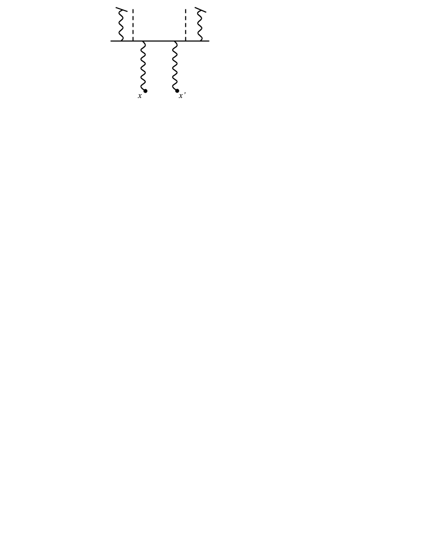
Figure 1: Symbolic diagrammatic picture of the effect of particle collisions and external electric field on the particle wave function. Wavy lines denote photon propagators, broken line the external electric field, solid lines charged particles.

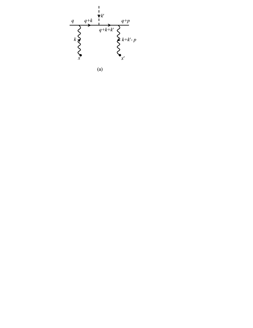
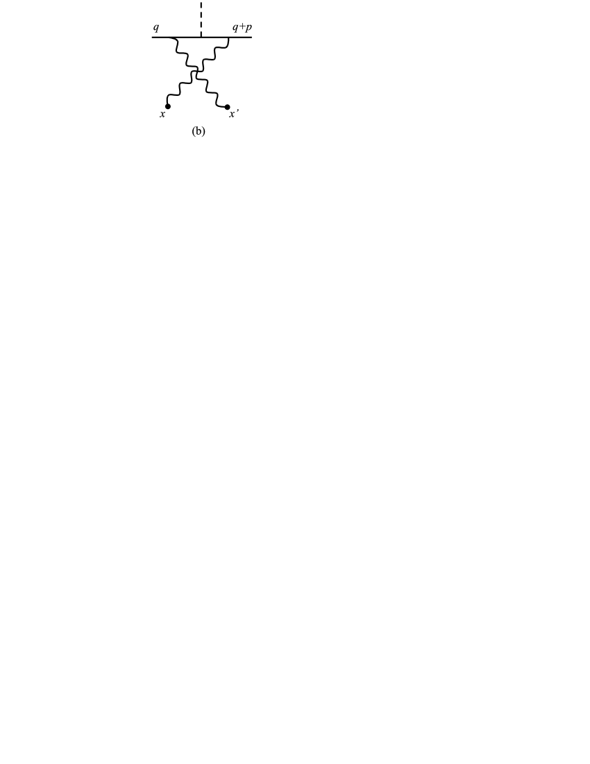
Figure 2: Feynman diagrams describing the first order external field correction to the particle propagator. $q$ and $p$ are the particle 4-momentum and 4-momentum transfer, respectively.

In this section, spectral density of the voltage correlation function will be evaluated in the low-frequency limit taking into account the finite-temperature effect and the influence of constant homogeneous external electric field. Let us first discuss the role of the particle collisions in this calculation. It was mentioned in Sec. II.1 that, barring the exchange interaction, correlations in the values of the electromagnetic fields produced by the charge carriers is a one-particle effect within the leading order in the electromagnetic coupling, in that only fields produced by one and the same particle correlate. At the same time, in the presence of the external electric field the direct particle interactions cannot be neglected completely. Indeed, although this field leads to a relatively small corrections to the charge carrier wave function and its propagator in all practically relevant cases, the effect of constant homogeneous field on the free-like particles cannot be treated perturbatively. The role of the particle collisions is to prevent the charge carrier from gaining too much momentum from the field, thus cutting down its effect. This is pictured schematically in Fig. 1 where the particle collisions are symbolized by a virtual photon interchange between the particles. The external field and the collisions affect both the particle wave function and its propagator. As to the former, account of these two factors is accomplished by replacing the particle momentum probability distribution by the statistical distribution function, obtained as a solution of the kinetic equation in the presence of external electric field (this point will be discussed in more detail later in this section). Regarding the particle propagator, however, the issue is not that simple, because in order to extract the low-frequency asymptotic of the power spectrum one needs an explicit expression for the propagator, incorporating both effects, which is unknown. This difficulty can be overcome by the following trick. As was mentioned above, the external field gives rise only to a relatively small correction to the particle propagator. It is, therefore, sufficient to determine this correction in the linear approximation, i.e., to the first order with respect to the electromagnetic coupling. We now make an assumption (confirmed by the result of the calculation) that the low-frequency asymptotic of the power spectrum is independent of the charge carrier mass. Then this asymptotic can be found formally in the large mass limit. For a given frequency $\omega,$ one can always take the mass large enough so as to justify perturbative treatment of the external field effect. To the first order in the electromagnetic coupling, corrections to the particle propagator due to external electric field and particle collisions are well-separated from each other because they are superimposed linearly. On the other hand, since the characteristic time of particle collisions is very small, their contribution to the particle propagator is inconsequential in calculating the low-frequency asymptotic of the power spectrum. Thus, the lowest order contribution to the correlation function is represented by diagrams with a single insertion of the vertex describing interaction of the charged particle with external electric field. These diagrams are shown in Fig. 2. Distinguishing the contributions of the diagrams 2(a) and 2(b) by the corresponding Latin subscript, we have

$$G_{a}(x,x^{\prime})=-e^{3}\iiint d^{4}zd^{4}z^{\prime}d^{4}z^{\prime\prime}A_{0}(z^{\prime\prime})$$

$$\times\left\{\mathfrak{D}(x-z)\left[\psi(z)\stackrel{{\scriptstyle\leftrightarrow}}{{\partial_{0}}}\mathfrak{D}^{\phi}(z-z^{\prime\prime})\stackrel{{\scriptstyle\leftrightarrow}}{{\partial_{0}^{\,\prime\prime}}}\mathfrak{D}^{\phi}(z^{\prime\prime}-z^{\prime})\stackrel{{\scriptstyle\leftrightarrow}}{{\partial_{0}^{\,\prime}}}\psi^{*}(z^{\prime})\right]\mathfrak{D}(z^{\prime}-x^{\prime})\right\}_{11}\,,$$ (21)

$$G_{b}(x,x^{\prime})=G_{a}(x^{\prime},x)\,,$$

where

$$\varphi\stackrel{{\scriptstyle\leftrightarrow}}{{\partial_{0}}}\psi = \varphi\partial_{0}\psi-\psi\partial_{0}\varphi\,,\quad\partial_{0}^{\,\prime}=\frac{\partial}{\partial z^{\prime}_{0}}\,,$$

$A_{0}(z^{\prime\prime})=-(\bm{E}\bm{z}^{\prime\prime})$ is the external field potential, and $\psi$ the given particle state. Next, we go over to momentum space with the help of Eqs. (9), (12), and introduce the spectral function for $G(x,x^{\prime})$ according to Eq. (II.3). Assuming also that the charged particle is nonrelativistic, and taking into account that $D^{\phi}_{12}=0,$ we write the matrix product longhand

$$G_{a}(\bm{x},\bm{x}^{\prime},t^{\prime},\omega)= (4\pi e)^{2}\iiint\frac{d^{3}\bm{q}}{(2\pi)^{3}}\frac{d^{\mathcal{D}}\bm{p}}{(2\pi)^{\mathcal{D}}}\frac{d^{\mathcal{D}}\bm{k}^{\prime}}{(2\pi)^{\mathcal{D}}}\psi(\bm{q})\psi^{*}(\bm{q}+\bm{p})$$ (22)

$$\times e^{ip^{0}(t^{\prime}-t_{0})-i(\bm{p}-\bm{k}^{\prime})\bm{x}^{\prime}}A_{0}(\bm{k}^{\prime})J_{a}(p,q,k^{\prime},\bm{x}-\bm{x}^{\prime},\omega)\,,$$

$$G_{b}(\bm{x},\bm{x}^{\prime},t^{\prime},\omega)= G^{*}_{a}(\bm{x},\bm{x}^{\prime},t^{\prime},-\omega)\,,\quad p^{0}=\frac{(\bm{q}+\bm{p})^{2}}{2m}-\frac{\bm{q}^{2}}{2m}\,,$$ (23)

where

$$J_{a}(p,q,k^{\prime},\bm{x}-\bm{x}^{\prime},\omega)= -\left.ie(2m)^{2}\int\frac{d^{\mathcal{D}}\bm{k}}{(2\pi)^{\mathcal{D}}}e^{i\bm{k}(\bm{x}^{\prime}-\bm{x})}\right.$$

$$\left.\times\left\{D_{11}(k)D^{\phi}_{11}(q+k)D^{\phi}_{11}(q+k+k^{\prime})D_{11}(k+k^{\prime}-p)\right.\right.$$

$$\left.\left.\hskip 14.22636pt-D_{12}(k)D^{\phi}_{22}(q+k)D^{\phi}_{22}(q+k+k^{\prime})D_{21}(k+k^{\prime}-p)\right\}\right|_{k_{0}=\omega},$$

$$A_{0}(\bm{k}^{\prime})= -i(2\pi)^{\mathcal{D}}\left(\bm{E}\frac{\partial}{\partial\bm{k}^{\prime}}\right)\delta^{({\mathcal{D}})}(\bm{k}^{\prime})\,,\quad k^{\prime}=(0,k_{1}^{\prime},k_{2}^{\prime},0)\,,\quad{\mathcal{D}}=2.$$

Here $q_{\mu}$ is the charged particle 4-momentum, and $\psi(\bm{q})$ its momentum wave function at some time instant $t_{0},$ normalized by

$$\int\frac{d^{3}\bm{q}}{(2\pi)^{3}}|\psi(\bm{q})|^{2}=1\,.$$ (25)

That the integrations over momenta $\bm{k},\bm{p},\bm{k}^{\prime}$ in the expressions (22), (III) turned out to be two-dimensional follows from the expression for the photon propagator, derived in the preceding section, which in the current notation can be written as

$$\mathfrak{D}(x)=\int\frac{d^{\mathcal{D}+1}k}{(2\pi)^{\mathcal{D}+1}}e^{-ikx}\mathfrak{D}(k)\,,\quad\mathcal{D}=2\,,$$

$\mathfrak{D}$ being given by Eq. (9). As we saw in Sec. II.1, this reduction of momentum space dimensionality from $\mathcal{D}=3$ to $\mathcal{D}=2$ is the consequence of quantum damping of temporal photon propagation in the $3$-direction. This suppression is noticeable only in sufficiently thin films with $a\lesssim r_{0},$ being formally complete in the practically unattainable case $a=d,$ and is negligible in thick samples with $a\gg r_{0}.$ To interpolate between these two limiting cases, it is natural to consider $\mathcal{D}$ in the above formulas as a phenomenological parameter allowed to take on non-integral values between $2$ and $3,$ and which therefore can be called “effective dimensionality” of the film. The difference $3-\mathcal{D}\equiv\delta$ thus will be an effective reduction of the film dimensionality, caused by the suppression. To accomplish this interpolation, we employ the well-known technique of dimensional continuation, developed by Wilson (in condensed matter theory), and by t’Hooft and Veltman (in quantum field theory) wilson .

Before evaluating the $\mathcal{D}$-integrals, let us note that the integrand in Eq. (III) can be considerably simplified. First of all, the second term in the curly brackets can be neglected. Indeed, in view of the factor $D_{12}(k)$ which is proportional to $\delta(k^{2}),$ and the condition $k_{0}=\omega,$ the momentum $k$ contributes only a tiny value to the argument of the factor $D_{21};$ for electrons in a crystal, for instance, the ratio $|\bm{k}|/|\bm{p}|\sim(\hbar\omega/c)/(\hbar/L)=\omega L/c\approx 10^{-10}\omega L,$ where $\omega,L$ are expressed in the $CGS$ system of units ($L$ is the sample length). Even for $L$ as large as $1\,{\rm cm},$ this ratio is very small for all practically relevant frequencies. Taking into account also that the momentum $\bm{k}^{\prime}$ is set eventually equal to zero, the factor $D_{21}(k+k^{\prime}-p)$ can be written simply as $D_{21}(p)\sim\delta(p^{2}).$ But the argument of this delta-function is always nonzero, because momentum transfer $p$ to the massive particle is spacelike. Furthermore, using explicit expression for the photon propagators, their product in the first term in the curly brackets reads

$$D_{11}(k)D_{11}(k+k^{\prime}-p)=\frac{1}{[k^{2}+i0]}\frac{1}{[(k+k^{\prime}-p)^{2}+i0]}-\frac{2\pi i\delta(k^{2})}{e^{\beta|k_{0}|}-1}\frac{1}{(k+k^{\prime}-p)^{2}+i0}$$

$$\hskip 113.81102pt-\frac{1}{k^{2}+i0}\frac{2\pi i\delta((k+k^{\prime}-p)^{2})}{e^{\beta|k_{0}-p_{0}|}-1}+\frac{2\pi i\delta(k^{2})}{e^{\beta|k_{0}|}-1}\frac{2\pi i\delta((k+k^{\prime}-p)^{2})}{e^{\beta|k_{0}-p_{0}|}-1}\,.$$

As before, the last term in this expression can be omitted, while the first term is dominated by the second, as we saw in Sec. II.2. Furthermore, $k_{0}$ enters the temperature exponent in the third term in the combination $(k_{0}-p_{0}),$ and therefore, this term does not contribute to the leading term of the low-frequency asymptotic, because in practice $|\omega|\ll p_{0}.$ Indeed, estimating the energy transfer $p_{0}$ as $(\bm{p}\bm{q})/m\approx\hbar^{2}/mdL,$ one finds for our standard example $|\omega/p_{0}|\sim 10^{-8}|\omega|L.$ Finally, in the product of the second term with $D^{\phi}_{11}(q+k)D^{\phi}_{11}(q+k+k^{\prime}),$ the pole of the function $D^{\phi}_{11}(q+k)$ does not contribute because of the factor $\delta(k^{2}).$ This is again a consequence of the requirement that the momentum transfer to the massive particle on-shell be spacelike: conditions $k^{2}=0,$ $q^{2}=m^{2},$ and $(q+k)^{2}=m^{2}$ cannot be satisfied altogether. Hence, the scalar particle propagator in this product can be written simply as $D^{\phi}_{11}(q+k)=-1/2(qk)\approx-1/2m\omega.$ Setting also $(e^{\beta|\omega|}-1)^{-1}\approx T/|\omega|,$ one thus finds

$$G_{a}(\bm{x},\bm{x}^{\prime},t^{\prime},\omega)= -i(2\pi)^{\mathcal{D}}(4\pi e)^{2}\iiint\frac{d^{3}\bm{q}}{(2\pi)^{3}}\frac{d^{\mathcal{D}}\bm{p}}{(2\pi)^{\mathcal{D}}}\frac{d^{\mathcal{D}}\bm{k}^{\prime}}{(2\pi)^{\mathcal{D}}}\psi(\bm{q})\psi^{*}(\bm{q}+\bm{p})$$

$$\times e^{ip^{0}(t^{\prime}-t_{0})-i(\bm{p}-\bm{k}^{\prime})\bm{x}^{\prime}}\left(\bm{E}\frac{\partial}{\partial\bm{k}^{\prime}}\right)\delta^{(\mathcal{D})}(\bm{k}^{\prime})J_{a}(p,q,k^{\prime},\bm{x}-\bm{x}^{\prime},\omega)\,,$$

where

$$J_{a}(p,q,k^{\prime},\bm{x}-\bm{x}^{\prime},\omega)=-\frac{4\pi emT}{\omega|\omega|}\int\frac{d^{\mathcal{D}}\bm{k}}{(2\pi)^{\mathcal{D}}}e^{i\bm{k}(\bm{x}^{\prime}-\bm{x})}\left.\frac{D^{\phi}_{11}(q+k+k^{\prime})\delta(k^{2})}{(k+k^{\prime}-p)^{2}+i0}\right|_{k_{0}=\omega}\,.$$

The singular at $\omega=0$ contribution to the function $G_{a}(\bm{x},\bm{x}^{\prime},t^{\prime},\omega)$ comes from integration over small $\bm{k}.$ The strength of this singularity is determined by the poles of the propagators in the integrand, and we have to decide which of them gives rise to the strongest singularity after performing the $\bm{k}^{\prime}$-integration. Consider first the case when the $\bm{k}^{\prime}$-derivative acts on the factors $[(k+k^{\prime}-p)^{2}+i0]^{-1},$ $e^{-i(\bm{p}-\bm{k}^{\prime})\bm{x}^{\prime}}.$ Since these depend on the difference $(\bm{p}-\bm{k}^{\prime}),$ changing $\partial/\partial\bm{k}^{\prime}\to-\partial/\partial\bm{p},$ and then integrating by parts with respect to $\bm{p}$ in Eq. (III), this derivative is rendered to act on terms independent of $\bm{k}.$ Thus, of all the $\bm{k}^{\prime}$-dependent factors in the integrand only $D^{\phi}_{11}(q+k+k^{\prime})$ is to be differentiated in effect. This brings the above expression for $G_{a}$ to the form

$$G_{a}(\bm{x},\bm{x}^{\prime},t^{\prime},\omega)= i(4\pi e)^{2}\iint\frac{d^{3}\bm{q}}{(2\pi)^{3}}\frac{d^{\mathcal{D}}\bm{p}}{(2\pi)^{\mathcal{D}}}\psi(\bm{q})\psi^{*}(\bm{q}+\bm{p})$$

$$\times e^{ip^{0}(t^{\prime}-t_{0})-i\bm{p}\bm{x}^{\prime}}\left(\bm{E}\bm{q}\right)J_{a}(p,q,\bm{x}-\bm{x}^{\prime},\omega)$$

with

$$J_{a}(p,q,\bm{x}-\bm{x}^{\prime},\omega)=-\frac{2\pi eT}{m\omega^{3}|\omega|\bm{p}^{2}}\int\frac{d^{\mathcal{D}}\bm{k}}{(2\pi)^{\mathcal{D}}}e^{i\bm{k}(\bm{x}^{\prime}-\bm{x})}\delta(\omega^{2}-\bm{k}^{2})\,.$$

It is seen from Eq. (18) that if a term in the function $C(\bm{x},\bm{x}^{\prime},t^{\prime},\omega)$ is independent of one of the arguments $\bm{x},$ $\bm{x}^{\prime},$ then it does not contribute to the voltage power spectrum. Hence, we expand the exponent in the integrand of (III), and retain only one term leading in the low-frequency limit. Using the rules of $\mathcal{D}$-integration wilson , one finds

$$J_{a}(p,q,\bm{x}-\bm{x}^{\prime},\omega) = \frac{\pi eT}{m\omega^{3}|\omega|\bm{p}^{2}}\int\frac{d^{\mathcal{D}}\bm{k}}{(2\pi)^{\mathcal{D}}}[\bm{k}(\bm{x}^{\prime}-\bm{x})]^{2}\delta(\omega^{2}-\bm{k}^{2})$$

$$= \frac{\pi eT(\bm{x}^{\prime}-\bm{x})^{2}}{m\omega^{3}|\omega|\bm{p}^{2}}\int\frac{d^{\mathcal{D}}\bm{k}}{(2\pi)^{\mathcal{D}}}\frac{\bm{k}^{2}}{\mathcal{D}}\delta(\omega^{2}-\bm{k}^{2})$$

$$= \frac{\pi eT(\bm{x}^{\prime}-\bm{x})^{2}}{m\omega^{3}|\omega|\bm{p}^{2}}\frac{|\omega|^{\mathcal{D}}S_{\mathcal{D}}}{2\mathcal{D}(2\pi)^{\mathcal{D}}}\,,$$

where

$$S_{\mathcal{D}}=\frac{2\pi^{\mathcal{D}/2}}{\Gamma(\mathcal{D}/2)}$$

is the area of unit hypersphere in $\mathcal{D}$ dimensional space ($\Gamma(x)$ is the Euler function). Thus,

$$G_{a}(\bm{x},\bm{x}^{\prime},t^{\prime},\omega)=\frac{i2\pi(4\pi)^{2-\mathcal{D}/2}}{\mathcal{D}\Gamma(\mathcal{D}/2)}\frac{e^{3}TL^{2}}{2m\omega|\omega|^{\delta}}\iint\frac{d^{3}\bm{q}}{(2\pi)^{3}}\frac{d^{\mathcal{D}}\bm{p}}{(2\pi)^{\mathcal{D}}}\psi(\bm{q})\psi^{*}(\bm{q}+\bm{p})e^{ip^{0}(t^{\prime}-t_{0})-i\bm{p}\bm{x}^{\prime}}\frac{(\bm{E}\bm{q})}{\bm{p}^{2}}\,,$$

where $L=|\bm{x}^{\prime}-\bm{x}|.$ The total contribution to the spectral density of the two-point Green function is

$$G(\bm{x},\bm{x}^{\prime},t^{\prime},\omega)=G_{a}(\bm{x},\bm{x}^{\prime},t^{\prime},\omega)+G^{*}_{a}(\bm{x},\bm{x}^{\prime},t^{\prime},-\omega)\,.$$

Substituting this into Eq. (20) one sees that since $G_{a}(\bm{x},\bm{x}^{\prime},t^{\prime},\omega)$ is odd with respect to frequency, it is the imaginary part of the Green function that contributes to the correlation function $C(\bm{x},\bm{x}^{\prime},t^{\prime},\omega)$ which therefore takes the form :

$$C(\bm{x},\bm{x}^{\prime},t^{\prime},\omega)=\frac{i2\pi(4\pi)^{2-\mathcal{D}/2}}{\mathcal{D}\Gamma(\mathcal{D}/2)}\frac{e^{3}TL^{2}}{m\omega|\omega|^{\delta}}{\rm Re}\iint\frac{d^{3}\bm{q}}{(2\pi)^{3}}\frac{d^{\mathcal{D}}\bm{p}}{(2\pi)^{\mathcal{D}}}\psi(\bm{q})\psi^{*}(\bm{q}+\bm{p})e^{ip^{0}(t^{\prime}-t_{0})-i\bm{p}\bm{x}^{\prime}}\frac{(\bm{E}\bm{q})}{\bm{p}^{2}}\,.$$

In a many-particle system, this result is to be expressed through the one-particle density matrix, which is accomplished by replacing $\psi^{*}(\bm{q}^{\prime})\psi(\bm{q})\to\varrho_{0}(\bm{q}^{\prime},\bm{q}),$ where $\varrho_{0}$ is the momentum space density matrix at the time instant $t_{0}.$ Recall that $t_{0}$ is the instant at which the particle state $\psi(\bm{q})$ is prepared. It can be identified, for instance, as the moment the charge carrier enters the sample, or escapes from a surface trap, etc. The factor $e^{ip_{0}(t^{\prime}-t_{0})}$ in the integrand realizes evolution of the density matrix from the instant $t_{0}$ to $t^{\prime}.$ Since $p_{0}=(\bm{q}+\bm{p})^{2}/2m-\bm{q}^{2}/2m,$ the product $e^{ip_{0}(t^{\prime}-t_{0})}\varrho_{0}(\bm{q}+\bm{p},\bm{q})$ describes a particle evolving freely on the interval $(t_{0},t^{\prime}).$ On the other hand, as was already mentioned in the beginning of this section, in order to justify perturbative treatment of the external field effect on the real particle states, it is necessary to take into account particle collisions. For this purpose, it is sufficient to consider these collisions as instantaneous. Then the interval $(t_{0},t^{\prime})$ is divided into a sequence of short time intervals of duration $\tau_{f}$ (the particle mean free time), on each of which the density matrix evolves freely, and changes abruptly at the collision instants. Going through this sequence, the density matrix tends to the stationary statistical distribution function, $\varrho(\bm{q}^{\prime},\bm{q}),$ which is independent of the initial particle state. What is important here is the sign of the difference $(t^{\prime}-t_{0}).$ Recall that $t^{\prime}$ is a fixed time instant to count off the time interval $\tau$ with respect to which the correlation function is Fourier-transformed, and that each particle has its own $t_{0}.$ This means that for a given $\omega,$ the system is observed during the time interval $(t^{\prime}-\Delta t,t^{\prime}+\Delta t),$ where $\Delta t\sim 1/\omega,$ and $t_{0}$s are distributed uniformly over this interval. The density matrix evolves forward (backward) in time, if $t^{\prime}>t_{0}$ ($t^{\prime}<t_{0}$). But time reversal involves inversion of particle momentum, and therefore, the reciprocal contributions to the function $G(\bm{x},\bm{x}^{\prime},t^{\prime},\omega)$ have opposite signs. To be more specific, let $(t^{\prime}-t_{0})>0.$ Then the exponent $e^{ip_{0}(t^{\prime}-t_{0})}$ realizes forward evolution of the density matrix, so that the integral in Eq. (III) takes eventually the form

$$\iint\frac{d^{3}\bm{q}}{(2\pi)^{3}}\frac{d^{\mathcal{D}}\bm{p}}{(2\pi)^{\mathcal{D}}}\varrho(\bm{q}+\bm{p},\bm{q})\frac{(\bm{E}\bm{q})}{\bm{p}^{2}}e^{-i\bm{p}\bm{x}^{\prime}}\,.$$ (27)

On the other hand, if $(t^{\prime}-t_{0})<0,$ then the density matrix evolves backward. In momentum space, the initial state of the reversed motion is represented by the amplitude $\tilde{\psi}(\bm{q})=\psi^{*}(-\bm{q}).$ Taking complex conjugate of the integral in Eq. (III) (which does not change the value of $G$ in view of the sign “Re”), and changing the integration variables $\bm{q}\to-\bm{q},$ $\bm{p}\to-\bm{p}$ gives in this case

$$-\iint\frac{d^{3}\bm{q}}{(2\pi)^{3}}\frac{d^{\mathcal{D}}\bm{p}}{(2\pi)^{\mathcal{D}}}\tilde{\psi}(\bm{q})\tilde{\psi}^{*}(\bm{q}+\bm{p})\frac{(\bm{E}\bm{q})}{\bm{p}^{2}}e^{ip_{0}(t_{0}-t^{\prime})-i\bm{p}\bm{x}^{\prime}}\,.$$

Replacing $\tilde{\psi}^{*}(\bm{q}+\bm{p})\tilde{\psi}(\bm{q})\to\tilde{\varrho}(\bm{q}+\bm{p},\bm{q}),$ where $\tilde{\varrho}$ plays the role of momentum density matrix at the moment $t^{\prime},$ the exponent $e^{ip_{0}(t_{0}-t^{\prime})}$ governs forward evolution of this state on the interval $(t^{\prime},t_{0}),$ so that the above expression takes the form

$$-\iint\frac{d^{3}\bm{q}}{(2\pi)^{3}}\frac{d^{\mathcal{D}}\bm{p}}{(2\pi)^{\mathcal{D}}}\varrho(\bm{q}+\bm{p},\bm{q})\frac{(\bm{E}\bm{q})}{\bm{p}^{2}}e^{-i\bm{p}\bm{x}^{\prime}}\,.$$

The density matrix here is the same as in (27), because the statistical distribution is independent of the initial state. We see that reciprocal contributions to the function $G(\bm{x},\bm{x}^{\prime},t^{\prime},\omega)$ cancel each other when summed over all particles in the system. Thus, we arrive at the important conclusion that the total noise intensity is independent of the number of particles, and remains at the level of individual contribution. As was shown in Ref. kazakov2 , this conclusion is also true of the disconnected part of the correlation function, though by virtue of quite different reasons.

It is customary to further express the function $\varrho(\bm{q}^{\prime},\bm{q})$ via the real mixed distribution function, $n(\bm{r},\bm{q}),$ according to

$$\varrho(\bm{q}+\bm{p},\bm{q})=\int d^{3}\bm{r}e^{i(\bm{p}\bm{r})}n\left(\bm{r},\bm{q}+\frac{\bm{p}}{2}\right)\,.$$

Probability distributions for the particle position in a sample or its momentum can be obtained by integrating $n(\bm{r},\bm{p})$ over all $\bm{p}$ or the sample volume, respectively. Using this in the expression (27), and substituting the latter into Eq. (III) yields

$$C(\bm{x},\bm{x}^{\prime},t^{\prime},\omega)=\frac{i2\pi(4\pi)^{2-\mathcal{D}/2}}{\mathcal{D}\Gamma(\mathcal{D}/2)}\frac{e^{3}TL^{2}}{m\omega|\omega|^{\delta}}{\rm Re}\iiint\frac{d^{3}\bm{q}}{(2\pi)^{3}}\frac{d^{\mathcal{D}}\bm{p}}{(2\pi)^{\mathcal{D}}}d^{3}\bm{r}\frac{(\bm{E}\bm{q})}{\bm{p}^{2}}n\left(\bm{r},\bm{q}+\frac{\bm{p}}{2}\right)e^{i\bm{p}(\bm{r}-\bm{x}^{\prime})}\,.$$

Shifting here $\bm{q}\to\bm{q}-\bm{p}/2,$ and dropping the purely imaginary term proportional to $(\bm{E}\bm{p}),$ the triple integral becomes purely real, so the symbol “${\rm Re}$” can be omitted. Integrating then over $\bm{p}$ with the help of the formula

$$\int\frac{d^{\mathcal{D}}\bm{p}}{(2\pi)^{\mathcal{D}}}e^{i(\bm{p}\bm{x})}\frac{4\pi}{\bm{p}^{2}}=\frac{\Gamma(\mathcal{D}/2-1)}{|\bm{x}|^{\mathcal{D}-2}\pi^{\mathcal{D}/2-1}}\,,\quad\mathcal{D}\neq 2$$

we obtain

$$C(\bm{x},\bm{x}^{\prime},t^{\prime},\omega)=\frac{2i(2\pi)^{\delta}}{\mathcal{D}(\mathcal{D}-2)}\frac{e^{3}TL^{2}}{m\omega|\omega|^{\delta}}\iint\frac{d^{3}\bm{q}}{(2\pi)^{3}}d^{3}\bm{r}(\bm{E}\bm{q})\frac{n(\bm{r},\bm{q})}{|\bm{r}-\bm{x}^{\prime}|^{\mathcal{D}-2}}\,.$$

Finally, substitution of this expression into Eq. (18) gives low-frequency asymptotic of the power spectrum of voltage fluctuations

$$C_{U}(\bm{x},\bm{x}^{\prime},t^{\prime},\omega)=-\frac{2i(2\pi)^{\delta}}{\mathcal{D}(\mathcal{D}-2)}\frac{e^{3}TL^{2}}{\omega|\omega|^{\delta}\Omega}\int d^{3}\bm{r}(\bm{E},\overline{\bm{v}}(\bm{r}))\left(\frac{1}{|\bm{r}-\bm{x}|^{\mathcal{D}-2}}+\frac{1}{|\bm{r}-\bm{x}^{\prime}|^{\mathcal{D}-2}}\right)\,,$$ (28)

where

$$\overline{\bm{v}}(\bm{r})=\Omega\int\frac{d^{3}\bm{q}}{(2\pi)^{3}}\frac{\bm{q}}{m}n(\bm{r},\bm{q})$$

is the local drift velocity of charge carriers, $\Omega$ denoting the sample volume. For a crystal in a homogeneous external field, $\overline{\bm{v}}$ is a function of the crystalline direction,

$$\overline{v}_{i}=\mu_{ik}E_{k}\,,\quad i,k=1,2,3,$$

where $\mu_{ik}$ is the charge carrier mobility tensor. To write down the final expression for the voltage power spectrum, we restore the ordinary units. Then Eq. (28) takes the form, for $\omega=2\pi f>0,$

$$C_{U}(\bm{x},\bm{x}^{\prime},t^{\prime},\omega)=-i\,\frac{\varkappa U^{2}_{0}}{f^{1+\delta}}\,,\quad\varkappa\equiv\frac{e^{3}c^{\delta}}{\pi\hbar^{2}c^{3}}\mu Tg\,,$$ (29)

where

$$\mu=\mu_{ik}n_{i}n_{k}\,,\quad\bm{n}=\frac{\bm{E}}{|\bm{E}|}\,,$$

$U_{0}=|\bm{E}|L$ is the voltage bias applied to the sample (it is assumed that $\bm{E}\parallel(\bm{x}-\bm{x}^{\prime}),$ as is usually the case in practice), and $g$ a geometrical factor

$$g=\frac{1}{\mathcal{D}(\mathcal{D}-2)a^{2\delta}\Omega}\int\limits_{\Omega}d^{3}\bm{r}\left(\frac{1}{|\bm{r}-\bm{x}|^{1-\delta}}+\frac{1}{|\bm{r}-\bm{x}^{\prime}|^{1-\delta}}\right)\,.$$ (30)

For $\omega<0,$ the sign of the right hand side in Eq. (29) is opposite. If Fourier transformation is defined in a purely real form, i.e., as a decomposition in $\cos(\omega\tau),$ $\sin(\omega\tau),$ rather than in $e^{i\omega\tau},$ then the spectral density is also real:

$$C_{U}(\bm{x},\bm{x}^{\prime},t^{\prime},\omega)=\frac{\varkappa U^{2}_{0}}{f^{1+\delta}}\,.$$ (31)

It is seen from Eq. (30) that the $g$-factor has a pole at $\mathcal{D}=2,$ which means that the noise amplitude is unbounded in the limit $\mathcal{D}\to 2.$ It was already mentioned in Sec. III that the case $\mathcal{D}=2$ would correspond to the practically unreachable film thickness $a=d.$ We now see that this case actually cannot be realized even theoretically. It should be emphasized in this connection that since in practice the film thickness always largely exceeds the lattice spacing, only a relatively small fraction of charge carriers in the film is correlated by the exchange interaction. Therefore, by continuity, the effective film dimensionality must be close to $3.$ In other words, the range of applicability of the developed theory is in any case limited to flicker noise spectra characterized by sufficiently small values of $\delta=\gamma-1.$

We mention for future reference that if the sample is an elongated (say, in $x$-direction) parallelepiped with the leads attached to its ends, then the $g$-factor can be evaluated approximately as

$$g\approx\frac{2}{\mathcal{D}(\mathcal{D}-2)a^{2\delta}Lwa}\int\limits_{0}^{L}\frac{wadx}{x^{1-\delta}}=\frac{2}{\delta\mathcal{D}(\mathcal{D}-2)a^{2\delta}L^{1-\delta}}\,,$$ (32)

where $w$ is the sample width, and it is assumed that $a<w\ll L.$ This is for $\delta>0.$ For $\delta$ close to zero, this formula is not applicable, because the $x$-integral diverges near the sample ends. Cutting off the integral at $x\approx w,$ one finds with logarithmic accuracy

$$g\approx\frac{2}{3Lwa}\int\limits_{w}^{L}\frac{wadx}{x}=\frac{2}{3L}\ln\frac{L}{w}\,,\quad\delta\approx 0\,.$$ (33)

We note also that in the $CGS$ system of units, the $\varkappa$-factor reads

$$\varkappa\approx 1.62\cdot 10^{10.48\,\delta-22}g\mu T\,,$$ (34)

where the absolute temperature $T$ is to be expressed in ${}^{\circ}{\rm K}.$

IV Applications

IV.1 Unboundedness of flicker noise spectrum

In this section, a special feature of the derived expression for the power spectrum, namely, its oddness in frequency, will be discussed in connection with the problem of observed absence of frequency limits of the $1/f^{\gamma}$-law. As was mentioned in Introduction, flicker noise has been detected in a very wide frequency band $\sim 10^{-6}\,{\rm Hz}$ to $10^{6}\,{\rm Hz}.$ This fact represents one of the essential difficulties for theoretical explanation, because all physical mechanisms underlying existing models of flicker noise work in much narrower subbands, and none of the models suggested so far has been able to explain the observed plenum of the $1/f$-spectrum.

On the other hand, existence of bounds on this spectrum is generally believed to be necessary in order to guarantee finiteness of the total noise power. There is a well-known argument flinn according to which these limits are actually unnecessary when the flicker noise exponent $\gamma$ is strictly equal to unity, because the logarithmic divergence of the total power is not a problem in this case in view of the existence of natural frequency cutoffs such as the inverse Planck time and lifetime of Universe. However, this reasoning does not work for $\gamma\neq 1,$ in which case divergence is a power of the cutoff. At the same time, the results obtained above reconcile unboundedness of $1/f$-spectrum with the requirements of stationarity and finiteness of the total noise power in a quite natural way. Indeed, using Eq. (29) we find that for $\delta<1$ the integral

$$\int\limits_{-\infty}^{+\infty}\frac{d\omega}{2\pi}C_{U}(\bm{x},\bm{x}^{\prime},t^{\prime},\omega)e^{i\omega\tau}=2i\int\limits_{0}^{+\infty}\frac{d\omega}{2\pi}C_{U}(\bm{x},\bm{x}^{\prime},t^{\prime},\omega)\sin(\omega\tau)=2\varkappa U^{2}_{0}\int\limits_{0}^{+\infty}df\frac{\sin(2\pi f\tau)}{f^{1+\delta}}$$

converges in both limits $f\to 0$ and $f\to\infty.$ In particular, the singular contribution to the voltage variance (i.e. to the quantity $C_{U}|_{\tau=0}$) vanishes. It is worth to note also that the total noise power would diverge for $\delta=1$ even if $\varkappa$ were bounded at $\mathcal{D}=2.$

Since appearance of odd contributions to the power spectrum is somewhat unusual in macroscopic fluctuation theory, let us discuss it in more detail. Under stationary external conditions, the voltage noise power spectrum (to be denoted below simply as $C_{U}(t,t^{\prime}),$ with the spatial arguments suppressed, for brevity) must be independent of $t^{\prime}.$ This is an expression of the noise stationarity, or, using a term more suitable for the subsequent discussion, time homogeneity with respect to the macroscopic system. It is usually realized as the requirement that $C_{U}(t,t^{\prime})$ be a function of the difference $t-t^{\prime}\equiv\tau.$ Since $C_{U}(t,t^{\prime})$ is also symmetric with respect to the interchange $t\leftrightarrow t^{\prime},$ an immediate consequence of this is that it is actually a function of $|\tau|,$ and hence the spectral density is a real even function of frequency. It is important, on the other hand, that time homogeneity is not necessarily exhibited by individual contributions to the total voltage fluctuation, whatever mechanism of flicker noise generation be. In particular, this property evidently does not take place at the microscopic level, i.e., with respect to elementary processes such as charge carrier trapping, surface or grain boundary scattering, etc. Stationarity of the macroscopic process emerges usually upon summation over a large number of individual contributions, so that this microscopic inhomogeneity turns out to be inconsequential. However, this summation is not the only way to obtain a stationary correlation function symmetric in $t,t^{\prime}.$ Another possibility, which is realized in the present paper, is that flicker noise may be a one-particle phenomenon, in the sense that the entire effect can be ascribed to elementary fluctuations produced by single charge carriers. In this case the function $C_{U}(t,t^{\prime})$ does not have to depend solely on $|\tau|,$ and as the explicit calculations of Sec. III show, it actually does not. As was mentioned above, elementary processes are inhomogeneous in time, and hence the symmetry with respect to $t\leftrightarrow t^{\prime}$ imposes no restriction on the $\tau$-dependence of the correlation function. The only remaining requirement, namely reality of the correlation function, implies that contributions to the spectral density must be real even, or imaginary odd functions of frequency [Cf. Eq. (20)]. These two cases correspond to the Fourier decomposition of the function $C_{U}(t^{\prime}+\tau,t^{\prime})$ in $\cos(\omega\tau)$ and $\sin(\omega\tau),$ respectively, and describe the parts symmetric and antisymmetric with respect to the difference of its time arguments. Finally, transition to the statistical distribution removes the $t^{\prime}$-dependence of the power spectrum [Cf. discussion after Eq. (III)]. This restores macroscopic time homogeneity of the correlation function, but leaves the possibility of being odd with respect to the difference of its time arguments. In other words, dependence of the power spectrum on $t^{\prime}$ shows itself only at microscopic scales, while macroscopically fluctuations look as if they were homogeneous in time.

The $1/f$-spectrum derived in the previous section has no lower frequency cutoff. As to the upper bound, it is given by the condition $f\ll T$ [see Sec. II.2], or in the ordinary units, $f\ll kT/\hbar\approx 10^{11}T\,{\rm Hz},$ with $T$ expressed in ${}^{\circ}{\rm K}.$ We see that from the practical point of view, the obtained spectrum has no upper cutoff either.

IV.2 Comparison with experimental data

Let us continue verification of the obtained result and show that Eq. (29) is in agreement with the other experimentally established properties of flicker noise. We will first discuss some general qualitative properties of flicker power spectra, predicted by Eq. (29), and then give a detailed quantitative comparison of these predictions with experimental data.

IV.2.1 Qualitative comparison with the experiment

First of all, the power spectrum of quantum electromagnetic fluctuations, given by Eq. (29), is quadratic in the applied bias. This is perhaps the most solidly established property of flicker noise. Second, the noise level is generally inversely proportional to the sample size. Namely, the $g$-factor describing dependence of the noise intensity on the sample dimensions increases roughly as a power of decreasing sample length or thickness, the exponent depending on the sample geometry as well as on the effective sample dimensionality $\mathcal{D}$ (which itself depends on the sample thickness.) As to the dependence of flicker noise amplitude on sample dimensions, agreement in the literature is not that good. Experiments are usually arranged so as to prove one of the two main competing points of view on the flicker noise origin, namely wether it is a bulk or surface effect. Although this issue is far from being resolved, there is no doubt that the noise level increases with decreasing sample size. To be more specific, we note that if $\delta={\rm const},$ then Eqs. (29), (32) tell us that the noise produced by an elongated sample is proportional to $a^{-2\delta}L^{\delta-1}.$ For experimental verification of this prediction we refer to wong1 ; wong2 which report the results of flicker noise measurements in various copper films with $a=400\,$Å$\div 2000\,$Å, and $L=800\,\mu{\rm m}\div 2000\,\mu{\rm m}.$ According to Ref. wong1 , the frequency exponent for samples on a silicon substrate exceeds noticeably that for equally sized samples on a sapphire substrate (the ratio of $\delta$’s for the two cases is about $1.5$). It follows then from the above formulas that the slope of the noise amplitude considered as a function of the film thickness is larger for samples on the silicon substrate. This is indeed the case as is clearly seen from Fig. 3 of Ref. wong1 . Furthermore, since $\delta$ increases for decreasing $a,$ the slope of the noise amplitude considered as a function of the sample length is expected to be larger for thicker samples, but with a less noticeable difference in the slopes since the length exponent $(\delta-1)$ is less sensitive to variations in $\delta$ than the thickness exponent $(-2\delta)$ ($\delta$ is about some tenths in both cases). This is again in agreement with the observations as is evident from Fig. 4 of Ref. wong1 where the amplitude curve for a $800\,$Å-thick film is somewhat steeper than that for a $400\,$Å-thick film (both on a silicon substrate).

Next, it is generally agreed that, with other things being equal, flicker noise is more intensive in semiconductors than in metals, and this is again in conformity with Eq. (29), because charge carrier mobility is higher in semiconductors than in metals, usually by several orders. Unfortunately, determination of mobility in semiconductors (or semimetals) is a difficult problem, both theoretically and experimentally, and different experiments often give significantly different results. By this reason, the subsequent consideration will be carried out for metals only. Even in this case careful estimation of the noise level takes some effort. This is because electron mobilities in thin metal films commonly used in flicker noise measurements differ essentially from the corresponding bulk values, varying non-monotonically with the film thickness, and exhibiting complicated temperature dependence. Thus, the thicker the film, the more reliable comparison of theoretical and experimental results. Fortunately, the modern instrumentation allows measurements in sufficiently thick samples, electrical transport in which has bulk properties (usually, effects related to film thickness become important for $h$ less than a few hundred nanometers). As is well known, temperature dependence of the electron mobility in this case is well approximated by the $1/T$ law. Theoretically, this approximation is valid for $T$ higher than the Debay characteristic temperature, but in most cases it is practically applicable already for $T\gtrsim 50^{\circ}{\rm K}.$ Furthermore, the effective dimensionality $\mathcal{D}\to 3$ in thick samples. Therefore, it follows from Eq. (29) that in sufficiently thick samples the frequency exponent $\gamma=1+\delta\approx 1,$ and the flicker noise level is temperature independent. This conclusion is confirmed, e.g., by the results of Ref. massiha where $1/f$ noise was measured in $2.44\,{\rm\mu m}$ thick metal films, which is quite sufficient for bulk treatment of the sample conduction. According to Fig. 5 of Ref. massiha , the flicker noise level is constant for $T\gtrsim 50^{\circ}{\rm K}$ indeed, and $\gamma$ is found to be about $1.01$ for most samples. In the opposite case of extremely thin films, conductivity is approximately independent of temperature. For instance, resistivity of a $5\,{\rm nm}$ thick gold film varies from the value $2.85\cdot 10^{-6}\Omega\cdot{\rm m}$ at $T=50\,^{\circ}{\rm K}$ to $3.0\cdot 10^{-6}\Omega\cdot{\rm m}$ at $T=275\,^{\circ}{\rm K},$ i.e., only by about $5\%$ pov . If $\delta=3-\mathcal{D}$ were constant, this would mean that the noise magnitude is a linear function of temperature in this case. However, $\delta$ is itself temperature dependent in thin films, namely, it is expected to decrease with increasing temperature, because thermal effects destroy the exchange correlations, thus raising the effective dimensionality of the sample.

Finally, it was found in wong1 that the frequency exponent in some cases depends also on the sample length, though much more weakly than on the sample thickness. This dependence cannot be explained from the point of view of the developed theory, so its appearance can serve as an indication on the limits of applicability of the theory.

IV.2.2 Quantitative comparison with the experiment

In order to compare the absolute value of the noise spectral density given by Eq. (29) with experimental data, we refer to the results of flicker noise measurements performed by Wong, Cheng and Ruan wong1 , which were used already in the above qualitative analysis, and by Voss and Clarke voss1 . Before going into detailed comparison, let us mention the following important circumstance. As is seen from Eq. (29), the noise amplitude is very sensitive to the value of $\delta.$ This parameter appears, in particular, in the exponent of the ratio $(c/fa^{2})$ which is normally very large. Indeed, for $f=1\,{\rm Hz}$ and $a=10^{-5}\,{\rm cm},$ this ratio is equal to $3\cdot 10^{20}.$ Therefore, an error as small as $0.01$ in the value of $\delta$ results in the extra factor of $10^{0.2}\approx 1.6$ in the amplitude. At the same time, $\delta$ is usually measured with the accuracy of a few hundredths at best, so the calculation carried out below is actually an order-of-magnitude estimation of the noise level.

Wong, Cheng and Ruan.

In this work, flicker noise power spectra were measured in the case of copper films of various thickness and length, sputtered on sapphire and oxidized silicon substrates. To illustrate the scheme of the calculation, let us take as an example the case of film with $L=1200\,\mu{\rm m},$ $a=1,2\cdot 10^{-5}\,{\rm cm},$ deposited on the sapphire wafer. According to Fig. 1 of wong1 , samples of this thickness have conductivity $\sigma=5.9\cdot 10^{6}\,\Omega^{-1}{\rm m^{-1}}.$ Using the relation $\mu=\sigma/en$ where $n=8\cdot 10^{22}\,{\rm cm}^{-3}$ is the charge carrier concentration in copper, one finds the electron mobility $\mu=1.4\cdot 10^{3}$ units CGS. Next, according to Fig. 5 of wong1 , the frequency exponent $\gamma$ in the case under consideration is equal to $1.1,$ hence, $\delta=\gamma-1=0.1.$ Substituting these values into the formula (32) gives $g=510$ units CGS. Finally, putting this and $T=300\,^{\circ}{\rm K}$ in Eq. (34), one obtains $\varkappa=3.8\cdot 10^{-13}.$ This value is to be compared with the measured value $\varkappa_{\rm exp}=6\cdot 10^{-13}$ given in Fig. 3 of Ref. wong1 (where it is called normalized noise amplitude). The experimental error of $\delta$ is about $0.02,$ which implies an ambiguity by the factor of $2.5$ in the calculated value of $\varkappa.$

It was found in wong1 that sufficiently thin copper films are characterized by a pronounced dependence of the frequency exponent on the sample length. Figure 5 of wong1 shows that the thinner the film, the stronger this dependence: for $L$ increasing from $800\,\mu{\rm m}$ to $2000\,\mu{\rm m},$ $\gamma$ decreases by only $0.05$ in the case of $a=800\,$Å, and by $0.15$ in the case of $a=400\,$Å. As was already mentioned above, the present theory is unable to explain this dependence, and hence the corresponding experimental data are beyond the scope of applicability of the theory. By this reason, the quantitative comparison below is carried out only for films with $a\geqslant 800\,$Å. The calculated and measured values of $\varkappa$ for films of various thickness on sapphire and silicon substrates are collected in Table I and Table II, respectively, together with the other parameters involved in the calculation. The quantities $\mu,g,\varkappa$ are given in the CGS system of units.

It is seen from these tables that the calculated and measured values of $\varkappa$ for films on sapphire wafer agree within the experimental error for all $a.$ For films on silicon wafer, the agreement within the experimental error is found for $a=1200\,$ Åand $a=1600\,$Å. In the case of $a=800\,$Å, where dependence of $\gamma$ on $L$ is still noticeable, the theory somewhat overestimates the noise level.

Voss and Clarke.

In the work voss1 , flicker noise was measured in thin metal films evaporated or sputtered on glass substrates. The information provided in this paper is sufficient for estimation of the noise intensity in the gold film shown in Fig. 2 of voss1 . This was an elongated sample with $h=25\,{\rm nm},$ $w=8\,{\rm\mu m},$ $l=625\,{\rm\mu m},$ biased at $U_{0}=0.81\,{\rm V},$ and operated at about $40^{\circ}{\rm K}$ above room temperature. Unfortunately, the exact value of $\gamma$ is not given for this case by the authors, who mentioned only that it is close to $1.$ In view of what have been said about dependence of the noise amplitude on $\delta,$ this implies a large amount of uncertainty in the theoretical estimation. Yet, assuming that $\delta\approx 0$ indeed, we substitute the sample dimensions in Eq. (33) and find $g=46\,{\rm cm}^{-1}.$ Next, in order to determine conductivity, we use the $I-V$ characteristic of the given gold sample, shown in Fig. 3 of voss1 . According to this figure, the sample resistance was about $100\,\Omega.$ Taking into account the sample dimensions given above, this implies that $\sigma=1.2\cdot 10^{6}\,{\rm\Omega^{-1}m^{-1}}.$ It should be mentioned that this value is approximately six times lower than that obtained in more recent studies of electrical transport in thin films. For instance, according to Ref. bieri conductivity of a $25\,{\rm nm}$ thick, $15\,{\rm\mu m}$ wide gold film obtained by a laser-improved deposition of nanoparticle suspension, is $7.1\cdot 10^{6}\,{\rm\Omega^{-1}m^{-1}}.$ The same value can be obtained also indirectly using the data given in Refs. chen ; pov . According to chen , the conductivity of gold is $75\%$ to $85\%$ of its bulk value for $h=100\,{\rm nm},$ depending on the choice of the substrate, and decreases below that value approximately linearly with decreasing thickness. On the other hand, according to Ref. pov conductivity drops to about $3\cdot 10^{5}\,{\rm\Omega^{-1}m^{-1}}$ for $h=5\,{\rm nm}.$ One readily finds from this that for $h=25\,{\rm nm},$ $\sigma=(6.5\div 7.5)\cdot 10^{6}\,{\rm\Omega^{-1}m^{-1}}.$ Presumably, this difference in the values of conductivity is to be attributed to the quality of film deposition. Substitution of $\sigma=1.2\cdot 10^{6}\,{\rm\Omega^{-1}m^{-1}}$ and $n=5.9\cdot 10^{22}\,{\rm cm}^{-3}$ in the relation $\mu=\sigma/en$ yields the electron mobility $\mu=390$ units CGS. Then Eq. (34) gives $\varkappa=9.6\cdot 10^{-16}$ (for $T=330\,^{\circ}{\rm K}$). Putting this together with the bias value given above in Eq. (29), we find $|C_{U}|=6.3\cdot 10^{-16}\,{\rm V^{2}/Hz}$ for the frequency $f=1\,{\rm Hz},$ which is to be compared with the experimental value $C_{U}\approx 10^{-15}\,{\rm V^{2}/Hz}\,.$

V Discussion and Conclusions

We have shown that, staying within the one-particle picture of flicker noise generation by quantum electromagnetic fluctuations, backreaction of the conducting medium on the fluctuating field of the charge carrier can be described phenomenologically as an effective reduction of the system dimensionality. Using the dimensional continuation technique, we have found that the backreaction affects both the frequency dependence and the magnitude of the noise spectrum. Namely, the frequency exponent in the $1/f^{\gamma}$-asymptotic of the fluctuation power spectrum in a conducting sample is found to be $1+\delta,$ where $\delta=3-\mathcal{D},$ $\mathcal{D}$ being the effective dimensionality of momentum space, while dependence of the noise amplitude on $\delta$ is given by Eqs. (29), (30). Although introduced initially as a momentum space characteristic, $\delta$ thus relates the noise amplitude to geometric properties of the sample in the ordinary $3$-dimensional coordinate space [Cf. Eqs. (30), (32)]. It was demonstrated in Sec. IV.2.1 that the experimentally observed dependence of the noise amplitude on the sample geometry for a given $\delta$ is adequately described by Eq. (32). The way $\delta$ itself depends on the sample thickness and system temperature, as expected from its definition, is also confirmed by observations. However, the value of $\delta$ cannot be predicted within the developed approach. In other words, $\delta$ plays the role of a phenomenological parameter of the theory. The noise amplitude turns out to be notably sensitive to the value of $\delta$: We saw in Sec. IV.2.2 that for a $10^{-5}\,{\rm cm}$-thick film, an increase of $0.1$ in $\delta$ raises the noise level by about two orders. This perfectly agrees with the observed rise of the noise level in samples with $\gamma>1$ in comparison with the predictions of the Hooge’s empirical formula hooge1 obtained for $\gamma=1.$ In fact, the quantitative comparison carried out in Sec. IV.2.2 shows that the calculated and measured values of the parameter $\varkappa$ coincide within the experimental error. Deviations between the theory and experiment become noticeable only in films with a pronounced dependence of the frequency exponent on the sample length. It was mentioned in Sec. IV.2.1 that this dependence cannot be explained from the point of view of the developed theory, so its appearance indicates the limits of applicability of the theory. Although this issue is beyond the scope of the present approach, it is yet worth to comment on the possible origin of these deviations. According to Ref. wong1 , dependence of the frequency exponent on the sample length is noticeable in sufficiently thin films. At the same time, the fact that films deposited on different substrates exhibit different noise characteristics clearly shows that the boundary conditions affect significantly the mechanism of noise generation. From the theoretical point of view, this is reflected in the essential role played by the assumption that the film is plane-parallel in the derivation of the photon propagator [Cf. discussion below Eq. (48)]. On the other hand, this assumption is violated to some extent by the surface roughness of the film. In fact, the authors of wong1 emphasize that the electric properties of the films used in their experiments are affected by the surface roughness, especially in the case of thin films. Thus, the surface roughness is a possible reason for the above-mentioned deviations in the values of $\varkappa.$

Finally, as was shown in Sec. IV.1, the obtained results explain the observed unboundedness of the flicker noise spectra, resolving naturally the problem of divergence of the total noise power. Together with the demonstrated qualitative and quantitative agreement of the results with experimental data, this suggests that quantum electromagnetic fluctuations is the source of flicker noise in metal films.

Appendix A Gauge independence of the power spectrum

Consider the theory of interacting scalar and electromagnetic fields described by the action

$$S=S_{\phi}+S_{A}\,,$$

where $S_{\phi}$ is given by Eq. (13), and

$$S_{A}=-\frac{1}{4}{\displaystyle\int}d^{4}xF_{\mu\nu}F^{\mu\nu}+S_{gf}\,,\quad S_{gf}=\frac{1}{2\alpha}{\displaystyle\int}d^{4}x~{}(\partial_{\mu}A^{\mu})^{2}\,,\quad F_{\mu\nu}=\partial_{\mu}A_{\nu}-\partial_{\nu}A_{\mu}\,.$$

For arbitrary constant parameter $\alpha,$ the gauge fixing term describes the generalized Lorentz gauge. Let us introduce the generating functional of Green functions

$$Z[J,\eta,\eta^{*}]=\int dAd\phi d\phi^{*}\exp\left\{i\left(S+\int d^{4}x[J^{\mu}A_{\mu}+\eta^{*}\phi+\eta\phi^{*}]\right)\right\}\,,$$ (35)

where $J,\eta,\eta^{*}$ denote sources for the fields $A,\phi^{*},\phi,$ respectively. Vanishing of $Z$ under the gauge variation of the functional integral variables

$$\delta A_{\mu}=\partial_{\mu}\xi(x)\,,\quad\delta\phi=ie\xi(x)\phi\,,\quad\delta\phi^{*}=-ie\xi(x)\phi^{*}\,,$$ (36)

with $\xi(x)$ a small gauge function, leads to the Ward identity

$$-i\partial_{\mu}J^{\mu}(y)Z+\frac{\Box}{\alpha}\partial_{\mu}\frac{\delta Z}{\delta J_{\mu}(y)}+ie\eta^{*}(y)\frac{\delta Z}{\delta\eta^{*}(y)}-ie\eta(y)\frac{\delta Z}{\delta\eta(y)}=0\,.$$ (37)

Since we are interested in the connected contribution to the correlation function, we rewrite this identity for the generating functional of connected Green functions, $W=-i\ln Z,$

$$-\partial_{\mu}J^{\mu}(y)+\frac{\Box}{\alpha}\partial_{\mu}\frac{\delta W}{\delta J_{\mu}(y)}+ie\eta^{*}(y)\frac{\delta W}{\delta\eta^{*}(y)}-ie\eta(y)\frac{\delta W}{\delta\eta(y)}=0\,.$$ (38)

The consequence of this equation we need is obtained by functional differentiation with respect to $\eta,\eta^{*},$ and twice with respect to $J,$ with all the sources set equal to zero afterwards,

$$\frac{\Box^{y}}{\alpha}\partial^{y}_{\mu}\frac{\delta^{5}W}{\delta J_{\mu}(y)\delta J_{\alpha}(x)\delta J_{\beta}(x^{\prime})\delta\eta(z)\delta\eta^{*}(z^{\prime})}+ie\delta^{(4)}(y-z^{\prime})\frac{\delta^{4}W}{\delta J_{\alpha}(x)\delta J_{\beta}(x^{\prime})\delta\eta(z)\delta\eta^{*}(y)}$$

$$-ie\delta^{(4)}(y-z)\frac{\delta^{4}W}{\delta J_{\alpha}(x)\delta J_{\beta}(x^{\prime})\delta\eta(y)\delta\eta^{*}(z^{\prime})}=0\,.$$

Fourier transform of this identity with respect to $y$ reads

$$\frac{k^{\prime 2}}{\alpha}k^{\prime}_{\mu}\int d^{4}ye^{-ik^{\prime}y}\frac{\delta^{5}W}{\delta J_{\mu}(y)\delta J_{\alpha}(x)\delta J_{\beta}(x^{\prime})\delta\eta(z)\delta\eta^{*}(z^{\prime})}$$

$$=e(e^{-ik^{\prime}z^{\prime}}-e^{-ik^{\prime}z})\frac{\delta^{4}W}{\delta J_{\alpha}(x)\delta J_{\beta}(x^{\prime})\delta\eta(z)\delta\eta^{*}(z^{\prime})}\,.$$ (39)

The argument of the Fourier transform is purposely denoted here by $k^{\prime}$ to stress that the left hand side of this equation corresponds to the variation of the Green function we dealt with in Sec. III, under gauge variation of the external field. Indeed, the longitudinal part of the photon propagator in the generalized Lorentz gauge has the form

$$D^{l}_{\mu\nu}(k)=-\alpha\frac{k_{\mu}k_{\nu}}{k^{4}}\,.$$ (40)

Therefore, contraction with the factor $k^{\prime 2}k^{\prime}_{\mu}/\alpha$ is equivalent to amputation of the photon propagator attached to the $y$ vertex, followed by contraction of this vertex with $k^{\prime}_{\mu}.$ Exactly the same result is obtained under the gauge variation of the external field coming into this vertex. The only difference with the Green function we considered in Sec. III is that the external scalar lines in Eq. (A) are the particle propagators. To promote them into particle amplitudes, according to the standard rules, Eq. (A) is to be Fourier transformed with respect to the variables $z,z^{\prime},$ and then multiplied by $\psi(\bm{q})\psi^{*}(\bm{q}^{\prime})(m^{2}-q^{2})(m^{2}-q^{\prime 2}),$ where the arguments $q,q^{\prime}$ of the Fourier transformations with respect to $z,z^{\prime}$ are to be taken eventually on the mass shell. But these operations give zero identically when applied to the right hand side of Eq. (A), because each of the factors $e^{-ik^{\prime}z^{\prime}},$ $e^{-ik^{\prime}z}$ makes the corresponding particle propagator nonsingular on the mass shell. For instance, the first term in Eq. (A) gives rise to the contribution of the form $(m^{2}-q^{\prime 2})D^{\phi}(q^{\prime}+k^{\prime})$ times terms nonsingular on the mass shell. For $k^{\prime}\neq 0,$ the function $D^{\phi}(q^{\prime}+k^{\prime})$ is also nonsingular at $q^{\prime 2}=m^{2},$ and hence this contribution vanishes on the mass shell.

Thus, the correlation function is invariant under gauge transformations of the external field, which are part of the gauge freedom in the theory. The other part is related to the explicit dependence of the photon propagator on the choice of the gauge conditions used to fix the gauge invariance of the action. As is well known, it is longitudinal part of the propagator that depends on the gauge. Let us first consider the simples case of Lorentz-invariant gauges. Then the most general form of the longitudinal part is given by Eq. (40) in which $\alpha$ is to be regarded as an arbitrary function of $k^{2}.$ It is not difficult to see that variations of $\alpha(k^{2})$ do not affect the observable quantities. Recall, first of all, that we are interested ultimately in the fluctuations of gauge-invariant quantities such as the electric field strength. The $\alpha$-independence of these quantities is a direct consequence of their gauge invariance, because variations of $\alpha(k^{2})$ give rise to terms that are pure gradients with respect to the spacetime arguments $x,x^{\prime},$ as is easily verified by substituting the expression (40) in place of one or two photon propagators in Eq. (III). Then, if the vector potential contribution to the field strength is negligible, as is the case in our nonrelativistic calculation (recall the condition $|\bm{q}|\ll m$ used throughout), the voltage correlation function can be found by integrating the correlation function for the field strength with respect to $\bm{x},\bm{x}^{\prime}$ using the relation $\bm{E}=-\bm{\nabla}A_{0}.$

More generally, the longitudinal part of the photon propagator in a Lorentz non-invariant gauge has the form, in coordinate space,

$$D^{l}_{\mu\nu}(x)=\partial_{\mu}\chi_{\nu}(x)+\partial_{\nu}\chi_{\mu}(x)\,,$$

where $\chi_{\mu}(x)$ is an arbitrary function of spacetime coordinates. If the Lorentz index of the spacetime derivative in $\partial_{\mu}\chi_{\nu}(x)$ is left free after combining the Feynman diagrams in Fig. 2, then this term leads to a gradient contribution to the two-point function of electromagnetic field, and, as before, does not contribute to the voltage correlation function. On the other hand, if the spacetime derivative is contracted with the interaction vertex, then the contribution of $\partial_{\mu}\chi_{\nu}(x)$ to the two-point function is not pure gradient, so the above argument does not work. Nevertheless, it can be shown that all such terms cancel each other in the complete expression for the correlation function. However, this requires examination of the complete set of Feynman diagrams, which complicates the proof. To avoid this complication, we will prove gauge independence of the low-frequency asymptotic of the power spectrum only, which is quite sufficient for our purposes. To this end, we use the following identity expressing invariance of the particle action under the transformation (36)

$$\frac{\delta S_{\phi}}{\delta\phi(x)}ie\phi(x)-\frac{\delta S_{\phi}}{\delta\phi^{*}(x)}ie\phi^{*}(x)-\partial^{x}_{\mu}\frac{\delta S_{\phi}}{\delta A_{\mu}(x)}=0\,.$$

Differentiating this identity twice with respect to $\phi(y),$ $\phi^{*}(z)$ and setting $A_{\mu}=0$ afterwards yields

$$\partial^{x}_{\mu}\frac{\delta^{3}S_{\phi}}{\delta A_{\mu}(x)\delta\phi(y)\delta\phi^{*}(z)}=\frac{\delta^{2}S_{\phi}}{\delta\phi(x)\delta\phi^{*}(z)}ie\delta^{(4)}(x-y)-\frac{\delta^{2}S_{\phi}}{\delta\phi^{*}(x)\delta\phi(y)}ie\delta^{(4)}(x-z)\,.$$

The left hand side here is just the interaction vertex contracted with the derivative coming from the term $\partial_{\mu}\chi_{\nu}(x).$ It follows that the result of this contraction is expressed through the inverse charged particle propagator. When built into the Feynman diagrams in Fig. 2, the latter is integrated with either the function $\psi(z)$ (the external line), or the particle propagator. In the first case it gives zero by virtue of the definition of free particle states, while in the second it cancels the particle propagator. At the same time, as we saw in Sec. III, it is singularity of the particle propagator that is responsible for the occurrence of $1/\omega$ contribution to the function $G(\bm{x},\bm{x}^{\prime},t^{\prime},\omega).$ Hence, longitudinal part of the photon propagator does not contribute to the leading low-frequency term of the power spectrum of electromagnetic fluctuations.

Thus, gauge-independence of our results expressed by Eqs. (28), (29) is proved completely.

Appendix B Photon propagator in thin metal film at $T=0.$

For the sake of clarity, we keep track of the factor $a$ in the formulas of the present section. As was mentioned in Sec. II.1, the only component of the photon propagator, relevant in the calculation of the two-point correlation function, is $D_{00}(x-x^{\prime})=i\langle\mathcal{T}\hat{A}_{0}(x)\hat{A}_{0}(x^{\prime})\rangle.$ This important fact will be proved below in the case of the axial gauge (2) which was seen to be particularly convenient in describing the damping of the temporal photon propagation in the $3$-direction. Let the unit vector in this direction be denoted by $n,$

$$n_{\mu}=-\eta_{3\mu}.$$

To determine the form of the photon propagator at zero temperature

$$D_{\mu\nu}(x-x^{\prime})|_{T=0}\equiv D^{0}_{\mu\nu}(x-x^{\prime})=\langle 0|\mathcal{T}\hat{A}_{\mu}(x)\hat{A}_{\nu}(x^{\prime})|0\rangle\,,$$ (41)

we go over to momentum space

$$D^{0}_{\mu\nu}(x)=\int\frac{d^{4}k}{(2\pi)^{4}}e^{-ikx}D^{0}_{\mu\nu}(k)\,,$$ (42)

and note that $D^{0}_{\mu\nu}(k)$ is a symmetric rank-two tensor that can be built only from the vectors $n_{\mu,}$ $k_{\mu},$ and the Minkowski tensor $\eta_{\mu\nu}.$ Therefore, it has the following general structure

$$D^{0}_{\mu\nu}(k)=\left\{\eta_{\mu\nu}+an_{\mu}n_{\nu}+b(k_{\mu}n_{\nu}+k_{\nu}n_{\mu})+ck_{\mu}k_{\nu}\right\}\Delta\,,$$

where $a,b,c,$ and $\Delta$ are some scalars built from $n_{\mu,}$ $k_{\mu},$ i.e., functions of the two invariant combinations $(nk)=-k_{3}$ and $k^{2}.$ According to discussion in Sec. II.1, the electromagnetic field operator $\hat{A}_{\mu}$ is constrained by $\hat{A}_{3}=0,$ $\partial\hat{A}_{0}/\partial x_{3}=0,$ which imply the following conditions on the form of the photon propagator

$$D_{3\nu}(x)=0\,,\quad\frac{\partial D_{0\nu}(x)}{\partial x_{3}}=0\,.$$ (43)

Written out in components, the first of these conditions reads

$$(bk_{0}+ck_{3}k_{0})\Delta = 0\,,$$

$$(bk_{i}+ck_{3}k_{i})\Delta = 0\,,\quad i=1,2\,,$$

$$(-1+a+2bk_{3}+ck^{2}_{3})\Delta = 0\,.$$

It follows that

$$b=-ck_{3}=c(nk)\,,\quad c=\frac{a-1}{k^{2}_{3}}=\frac{a-1}{(nk)^{2}}\,,$$

so

$$D^{0}_{\mu\nu}(k)=\left\{\eta_{\mu\nu}+an_{\mu}n_{\nu}+(a-1)\frac{(k_{\mu}n_{\nu}+k_{\nu}n_{\mu})}{(nk)}+(a-1)\frac{k_{\mu}k_{\nu}}{(nk)^{2}}\right\}\Delta\,.$$ (44)

Then the second of the conditions (43) gives

$$\left\{(nk)\eta_{0\nu}+(a-1)k_{0}n_{\nu}+(a-1)\frac{k_{0}k_{\nu}}{(nk)}\right\}\Delta=0\,.$$

The $3$-component of this condition is satisfied identically, while the other three yield

$$\left\{(nk)+(a-1)\frac{k^{2}_{0}}{(nk)}\right\}\Delta = 0\,,$$ (45)

$$(a-1)\frac{k_{0}k_{i}}{(nk)}\Delta = 0\,,\quad i=1,2\,.$$ (46)

Since the photon propagator does depend on $x_{0},x_{1},x_{2},$ it follows form Eq. (46) that $a=1,$ and then Eq. (45) gives $k_{3}\Delta=0$ implying that the function $D^{0}_{\mu\nu}(x)$ is independent of $x_{3}.$ Thus,

$$D^{0}_{\mu\nu}(k)=\left(\eta_{\mu\nu}+n_{\mu}n_{\nu}\right)\Delta\,.$$ (47)

It remains only to find the quantity $\Delta.$ To this end, we will calculate the $00$-component of the propagator explicitly.

Under the condition $\partial\hat{A}_{0}/\partial x_{3}=0,$ the normal mode decomposition of the scalar potential operator reads

$$\hat{A}_{0}(\bm{x},t)=N\sum\limits_{k_{1},k_{2}}\frac{1}{\sqrt{2\omega_{k}}}\left(\hat{a}_{\bm{k}}\exp\{i(-\omega_{k}t+k_{1}x_{1}+k_{2}x_{2})\}+{\rm H.c.}\right)\,,\quad\omega_{k}=|\bm{k}|\,,$$

where $N$ is a normalization factor to be determined below, and $\hat{a}_{\bm{k}}$ is the annihilation operator of a “temporal” photon with the wave vector $\bm{k}=(k_{1},k_{2},0).$ As is known from quantum electrodynamics, the commutator of this operator with its Hermitian conjugate is $\hat{a}_{\bm{k}}\hat{a}^{\dagger}_{\bm{k}}-\hat{a}^{\dagger}_{\bm{k}}\hat{a}_{\bm{k}}=-1\,.$ Substituting the expression for $\hat{A}_{0}$ in Eq. (41), one finds

$$D^{0}_{00}(\bm{x},t)=-N^{2}\sum\limits_{\bm{k}}\frac{i}{2|\bm{k}|}\exp\{i(-\omega_{k}|t|+\bm{k}\bm{x})\}\,.$$

As always, the factor $N$ depends on the choice of a “box” in which the field is quantized. Suppose that this box is a rectangular in $(x_{1},x_{2})$-plane, its sides being parallel to the coordinate axes. For a sufficiently large box, summation over $\bm{k}$ can be replaced by integration over $Sd^{2}\bm{k}/(2\pi)^{2},$ where $S$ is the box area,

$$D^{0}_{00}(\bm{x},t)=-iN^{2}S\int\frac{d^{2}\bm{k}}{(2\pi)^{2}}\frac{e^{i(-\omega_{k}|t|+\bm{k}\bm{x})}}{2|\bm{k}|}=N^{2}S\int\limits_{-\infty}^{+\infty}\frac{dk_{0}}{2\pi}\int\frac{d^{2}\bm{k}}{(2\pi)^{2}}\frac{e^{i(-k_{0}t+\bm{k}\bm{x})}}{k^{2}_{0}-\bm{k}^{2}+i0}\,.$$

$N$ can be found by calculating the electric potential produced by a resting point charge, $e.$ If this charge is at the origin of the coordinate system, then the potential at the point $\bm{x}=(x_{1},x_{2},0)$ is given by the well-known formula

$$A_{0}(\bm{x})=-e\int\limits_{-\infty}^{+\infty}dtD^{0}_{00}(\bm{x},t)\,.$$

Substitution of the explicit expression for $D^{0}_{00}(\bm{x},t)$ yields

$$A_{0}(\bm{x})=eN^{2}S\int\frac{d^{2}\bm{k}}{(2\pi)^{2}}\frac{e^{i\bm{k}\bm{x}}}{\bm{k}^{2}}\,.$$ (48)

On the other hand, since this potential is independent of $x_{3},$ the same result will be obtained if the film is replaced by an infinite set of identical parallel films adjacent to each other. This is allowed by our assumption that the film is plane-parallel. In other words, $A_{0}(\bm{x})$ can be represented as a superposition of the Coulomb potentials produced by an infinite sequence of vertically aligned point charges, spaced at the distance $a,$ or equivalently, by a charge distribution with density $\rho(x_{1},x_{2},x_{3})=(e/a)\delta^{(2)}(x_{1},x_{2}).$ Fourier transform of the latter is $\rho(\bm{k})=(e/a)2\pi\delta(k_{3}),$ hence

$$A_{0}(\bm{x})=\int d^{3}\bm{x}^{\prime}\frac{\rho(\bm{x}^{\prime})}{|\bm{x}-\bm{x}^{\prime}|}=\int\frac{d^{3}\bm{k}}{(2\pi)^{3}}\rho(\bm{k})\frac{4\pi e^{i\bm{k}\bm{x}}}{\bm{k}^{2}}=\frac{4\pi e}{a}\int\frac{d^{2}\bm{k}}{(2\pi)^{2}}\frac{e^{i\bm{k}\bm{x}}}{\bm{k}^{2}}\,,$$

and comparison with the preceding formula gives

$$N=\sqrt{\frac{4\pi}{Sa}}\,.$$

The $00$-component of the photon propagator thus takes the form

$$D^{0}_{00}(x)=\int\frac{d^{4}k}{(2\pi)^{4}}e^{-ikx}\Delta\,,\quad\Delta=\frac{8\pi^{2}}{a}\frac{\delta(k_{3})}{k^{2}+i0}\,.$$

Putting this $\Delta$ in Eqs. (47), (42), we arrive finally at the following expression for the zero-temperature photon propagator

$$D^{0}_{\mu\nu}(x)=\left(\eta_{\mu\nu}+n_{\mu}n_{\nu}\right)\frac{1}{a}\int\frac{d^{3}k}{(2\pi)^{3}}e^{-ikx}\frac{4\pi}{k^{2}+i0}\,.$$

$a,$ Å	$\delta$	$\mu\times 10^{-3}$	$G\times 10^{-2}$	$\varkappa_{\rm th}\times 10^{13}$	$\varkappa_{\rm exp}\times 10^{13}$
800	0.14	1.1	9.8	15	9
1200	0.10	1.4	5.1	3.8	6
1600	0.10	2.2	4.7	5.5	5

Table 1: Calculated ($\varkappa_{\rm th}$) and measured ($\varkappa_{\rm exp}$) values of $\varkappa$ for copper films of various thickness on sapphire substrates. $\mu,g,\varkappa$ are given in the CGS system of units.

$a,$ Å	$\delta$	$\mu\times 10^{-3}$	$G\times 10^{-2}$	$\varkappa_{\rm th}\times 10^{12}$	$\varkappa_{\rm exp}\times 10^{12}$
800	0.21	0.9	32	22	2
1200	0.17	1.2	14	4.9	2
1600	0.14	2.0	8	2.3	1

Table 2: Same for copper films on silicon substrates.

.

References

- (1) See, for instance, M. Buckingham, Noise in Electronic Devices and Systems (Chichester: Ellis Horwood, 1983). Recent reviews of the problem can be found in Ref. wong2 ; A. K. Raychaudhuri, Current Opinion in Solid State & Materials Science 60, 67 (2002); E. Milotti, physics/0204033, and references therein. General mathematical description of noise can be found in B. Kaulakys, V. Gontis, and M. Alaburda, Phys. Rev. E71, 051105 (2005), which also contains an extensive bibliography. An up-to-date bibliographic list on -noise can be found at http://www.nslij-genetics.org/wli/1fnoise.
- (2) J. B. Johnson, Phys. Rev. 26, 71 (1925); 29, 367 (1927).
- (3) R. F. Voss and J. Clarke, Phys. Rev. B13, 556 (1976).
- (4) J. Clarke and T. Y. Hsiang, Phys. Rev. Lett. 34, 1217 (1975).
- (5) F. N. Hooge, Physica (Utr.) 60, 130 (1972).
- (6) F. N. Hooge, Phys. Lett A 29, 139 (1969); F. N. Hooge and A. M. H. Hoppenbrouwers, Physica (Utr.) 45 , 386 (1969).
- (7) Th. G. M. Kleinpenning, Physica (Utr.) 77, 78 (1974).
- (8) Th. G. M. Kleinpenning and D. A. Bell, Physica (Utr.) 81B, 301 (1976).
- (9) L. K. J. Vandamme and Gy. Trefan, Fluctuation and Noise Lett. 1, R175 (2001).
- (10) D. A. Bell, Proc. Phys. Soc. 72, 27 (1958).
- (11) A. L. McWhorter, In Semiconductor Surface Physics, ed. R. H. Kingston (University of Pennsylvania, Philadelphia, 1957), p. 207.
- (12) A. van der Ziel, Appl. Phys. Lett. 33, 883 (1978).
- (13) A. van der Ziel, Advances in Elect. and Phys. 49, 225 (1979).
- (14) Th. G. M. Kleinpenning, J. Appl. Phys. 51, 3438 (1980).
- (15) B. K. Jones, Proc. 6th Int. Conf. on Noise in Physical Systems, Gaithersburg, MD, USA (1981) p. 206.
- (16) V. B. Orlov and A. V. Yakimov, Physica B 162, 13 (1990).
- (17) J. F. Stephany, J. Phys.: Condens. Matter 12, 2469 (2000).
- (18) P. H. Handel, Phys. Rev. Lett. 34, 1492 (1975); Phys. Rev. A22, 745 (1980). A fairly complete bibliography on the quantum theory approach to -noise can be found at http://www.umsl.edu/ handel/QuantumBib.html
- (19) P. H. Handel, IEEE Trans. on Electron. Devices 41, 2023 (1994); Phys. Stat. Sol. (b)194, 393 (1996); in Wiley Encyclopedia of Electrical and Electronics Engineering, Ed.: John G. Webster, Vol. 14, pp. 428-449 (John Wiley & Sons, 1999).
- (20) A.-M. Tremblay, PhD thesis, Massachusetts Institute of Technology, 1978; Th. M. Nieuwenhuizen, D. Frenkel and N. G. van Kampen, Phys. Rev. A35, 2750 (1987).
- (21) C. M. Van Vliet, Physica A 165, 101,126 (1990).
- (22) A. van der Ziel, “Unified Presentation of 1/f Noise in Electronic Devices: Fundamental 1/f Noise Sources”, Proc. IEEE 76, 233 (1988); J. Appl. Phys. 63, 2456 (1988).
- (23) K. A. Kazakov, Int. J. Mod. Phys. B 20, 233 (2006); J. Phys. A: Math. and Gen. 39, 7125 (2006).
- (24) K. A. Kazakov, J. Phys. A: Math. and Theor. 39, 7125 (2007).
- (25) L. D. Landau and E. M. Lifshitz, Statistical Physics. Part 1. (Pergamon, New York, 1980).
- (26) J. Schwinger, J. Math. Phys. 2, 407 (1961); Particles, Sources and Fields (Addison-Wesley, Reading, Mass., 1970)
- (27) L. V. Keldysh Zh. Eksp. Teor. Fiz. 47, 1515 (1964) [Sov. Phys. JETP 20, 1018 (1965)].
- (28) N. P. Landsman and Ch. G. van Weert, Phys. Reports 145, 141 (1987).
- (29) A. J. Niemi and G. W. Semenoff, Ann. Phys. 152, 105 (1984); Nucl. Phys. B 230 [FS10], 181 (1984).
- (30) K. G. Wilson, Phys. Rev. D 7, 2911 (1973); G. t’Hooft and M. Veltman, Nucl. Phys. B 44, 189 (1972). A comprehensive account of the dimensional continuation techniques can be found in J. C. Collins, Renormalization (Cambridge University Press, 1984).
- (31) I. Flinn, Nature 219, 1356 (1968).
- (32) H. Wong, Y. C. Cheng, and G. Ruan, J. Appl. Phys. 67, 312 (1990).
- (33) H. Wong, Microelectron. Reliab. 43, 585 (2003).
- (34) G. H. Massiha and K. S. Rawat, J. Ind. Technol. 18, 1 (2002).
- (35) G. Chen et al., Appl. Phys. A 80, 659 (2005).
- (36) A. Povilus, Electronic properties of metals and semiconductors, (Michigan Univ. Report N 441, 2003).
- (37) N. R. Bieri et al., Superlattices and Microstructures 35, 437 (2004).