Viable flux distribution in metabolic networks

Abstract

The metabolic networks are very well characterized for a large set of organisms, a unique case in within thelarge-scale biological networks. For this reason they provide a a very interesting framework for the construction of analytically tractable statistical mechanics models. In this paper we introduce a solvable model for the distribution of fluxes in the metabolic network. We show that the effect of the topology on the distribution of fluxes is to allow for large fluctuations of their values, a fact that should have implications on the robustness of the system.

1 Introduction

Dynamical models on networks have attracted a large interest because of the non-trivial effects of network structure RMP ; Doro ; Newman ; Internet on the dynamics defined on them Critical . Important examples of the dynamics on networks with relevant applications are the Ising model Doro_Ising ; Diluito ; annealed , the spreading of a disease Vespi_epi and the synchronization models Motter ; Moreno . In this paper introduce a solvable model for the distribution of fluxes in the metabolic network. While motivations come from the study of the metabolic network, the problem is quite general and can be applied to supply networks and to many other linear problems Linear of constraint satisfaction on continuous variables on a network.

Metabolic networks describe the stoichiometric relations between substrates in biochemical reactions inside the cell. They have been mapped BIGG for a large number of organisms in the three different domains of life (archea, bacteria and eukaryotes). They provide the biomass needed for cell duplication, and the rate of biomass production (growth rate) can be identified with a fitness of the cell. The structure of the metabolic network can be represented as a factor graph with nodes that are chemical reactions and function nodes that are chemical metabolites. The projection of the network on the metabolites has a power-law degree distribution and a hierarchical structure metabolic ; modularity ; Tanaka . To each factor node, which describes a chemical reactions, it is associated an enzyme which itself is produced by a regulated gene network. Important aspect of the functioning of these very complex systems include dynamical considerations. Flux-balance-analysis fba ; Palsson ; Palsson2 make a major semplification in the problem. In fact it considers only the steady state of the dynamics and includes all the dynamical terms inside the definition of the flux of a reaction. For this reason it was able to predict with sufficient accuracy the fluxes of the reactions in the graph for a given environmentand it consitute a real break-through in the field. Special interest has been addressed to the perturbation of the distribution of the fluxes after knockout of a gene or in different environments MOMA ; ROOM . The problem of identifying the flux distribution in Escherichia coli was studied experimentally exp and by means of Flux-Balance-Analysis Almaas . A fat tail in their distribution with different power-law exponents $\alpha<2$ was found.

Metabolic networks provide a very interesting framework for the construction of analytically tractable models using tools of statistical mechanics of disordered systems. In this paper we will discuss the impact of the network structure (degree distributions) on the steady state distribution distribution of the fluxes. We shall consider random networks with the same degree distribution as the real ones i.e. networks in the the hidden-variable ensemble hv1 ; hv2 ; hv3 with same expected degree distribution as the metabolic factor graphs. Formally the problem is resolved with replica calculations on diluted networks Diluito extended to the case of continuous variables. Due the simplicity of the Hamiltonian the problem is solved with an expansion of the order parameter in terms of Gaussians. The problem shares some similarity with other problems in statistical mechanics of disordered systems Localized ; Guil . In a recent paper DeMartino a similar problem was considered in the framework of a different model where the steady state of the fluxes is not a priori considered and the positive fluxes don’t have any upper limit.

2 The model

The metabolic network has a bow tie structure Tanaka : the metabolites are divided into: (i) input metabolites which are provided by the environment, (ii) the output metabolites which provide the biomass and (iii) the intermediate metabolites. The stochiometric matrix is given by $((\xi_{\mu,i}))$ where $\mu=1,\dots,M$ indicates the metabolite and $i=1,\dots,N$ the reaction and the sign of $\xi_{\mu,i}$ indicates if the metabolite $\mu$ is an input or output metabolite of the reaction $i$. As in the Flux-Balance-Analysis method we assume that each intermediate metabolite has a concentration $c_{\mu}$ which is consumed/produced by a reaction $i$ at a rate $f_{i}$. At steady state, we have

$$\frac{dc_{\mu}}{dt}=\sum_{i}\xi_{\mu,i}f_{i}=a^{\mu}=0$$ (1)

where $f_{i}$ is the flux of the metabolic reaction $i$. For the metabolites present in the environment and the metabolites giving rise to the biomass production we can fix the incoming flux given by

$$\frac{dc_{\mu}}{dt}=\sum_{i}\xi_{\mu,i}f_{i}=a^{\mu}_{in/out}.$$ (2)

The fluxes in Eqs.(1-2) can vary inside a fixed volume $\Omega$. We assume for simplicity that this volume is an hypercube $\Omega=[0,2L]^{N}$. Changing the variables $f_{i}$ in the variables $s_{i}=f_{i}-L$ and the equations that the fluxes $s_{i}$ must satisfy are given by

$$\sum_{i=1}^{N}\xi_{\mu,i}s_{i}=g_{\mu}\ \mbox{for}\ \mu=1,\dots M.$$ (3)

where $g_{\mu}=a^{\mu}-L\sum_{i}\xi_{\mu,i}$. The volume of solutions $V$, given the constraints $(\ref{uno})$, is proportional to the quantity

$$\tilde{V}=\int_{0}^{L}dL^{\prime}\int\prod_{i=1}^{N}ds_{i}\delta(\sum_{i}\xi_{\mu,i}s_{i}-g^{\mu})\delta(\sum_{j}q_{j}s_{j}^{2}-\langle{q_{i}}\rangle NL^{\prime 2}).$$ (4)

where we have used the heterogeneous spherical constraints

$$\frac{1}{\langle{q_{i}}\rangle N}\sum_{i}q_{i}s_{i}^{2}=L^{\prime 2}$$ (5)

and integrated over $L^{\prime}$ in the interval $[0,L]$ in order to allow analytical treatment of the problem.

3 Replica method

We assume that the support of our stochiometric matrix is a random network with given degree distribution, i.e. a realization of the random hidden-variable model hv1 ; hv2 ; hv3 . In particular we fix the expected degree distribution of the nodes of the factor graphs to be $q_{i}$ for the reaction node $i=1,\dots N$ and $q_{\mu}$ for the metabolite nodes $\mu=1,\dots,M$ and we assume that the matrix elements $\xi_{\mu,i}$ are distributed following

$$P(\xi_{\mu,i})=\frac{q_{i}q_{\mu}}{2\langle{q_{i}}\rangle N}\left[\delta(\xi_{\mu,i}-1)+\delta(\xi_{\mu,i}+1)\right]+\left(1-\frac{q_{i}q_{\mu}}{\langle{q_{i}}\rangle N}\right)\delta(\xi_{\mu,i}),$$ (6)

where $\delta()$ indicates the Kronecker delta. Note that in $(\ref{pxi})$ we have assumed that the elements of the stochiometric matrix have values $0,\pm 1$ with a random sign and that the variables $q_{i}$ $q_{\mu}$ are nothing else than the hidden-variables associated with metabolite $\mu$ of the reaction $i$ of the hidden-variable network ensemble hv1 ; hv2 ; hv3 .

In order to evaluate the steady state distribution of the fluxes in a typical network realization we replicate the realizations of the $s_{i}^{a}$ and we compute $\langle{\log({V})}\rangle$ over the different network realizations. To calculate this average we use the replica trick $S=\langle{\log({Z})}\rangle=\lim_{n\rightarrow 0}\frac{\langle{\tilde{V}^{n}}\rangle-1}{n}$. The averaged unormalized volume of solutions $<\tilde{V}^{n}>$ can be expressed as

$$<\tilde{V}^{n}>=\int_{0}^{L}dL^{\prime}\int\prod_{a}d{\omega^{a}}\int\prod_{a,i}ds_{i,a}\int\prod_{a,\mu}d\lambda_{\mu,a}\exp\left[-ig_{\mu}\sum_{a}\lambda_{\mu,a}\right]$$

$$\exp\left[-\sum_{i,\mu}\frac{q_{i}q_{\mu}}{\langle{q_{i}}\rangle N}(1-\cos{\vec{\lambda}}_{\mu}\cdotp\vec{s}_{i})+i\sum_{a}\omega^{a}\left(\sum_{j}q_{j}s_{j,a}^{2}-L^{\prime 2}\langle{q_{i}}\rangle N\right)\right].$$ (7)

Using the techniques coming from the field of diluted systems, we introduce the order parameters Order ; Diluito

$$c(\vec{\lambda})=\frac{1}{\langle{q_{i}}\rangle N}\sum_{\mu}q^{\mu}\prod_{a}\delta(\lambda_{\mu}^{a}-\lambda^{a})$$

$$c(\vec{s})=\frac{1}{\langle{q_{i}}\rangle N}\sum_{i}q^{i}\prod_{a}\delta(s_{i}^{a}-s^{a})$$ (8)

getting for the volume

$$\left\langle{\tilde{V}^{n}}\right\rangle=\int{\cal D}c(\vec{\lambda})\int{\cal{D}}\hat{c}(\vec{\lambda})\int{\cal D}c(\vec{s})\int{\cal{D}}\hat{c}(\vec{s})\exp[nN\Sigma(\hat{c}(\vec{\lambda}),c(\vec{\lambda}),\hat{c}({\vec{s}}),c({\vec{s})})]$$

with

$$n\Sigma = \int d\vec{\lambda}i\hat{c}(\vec{\lambda})c(\vec{\lambda})+\int d\vec{s}i\hat{c}({\vec{s}}){c}({\vec{s}})-\int d\vec{\lambda}\int d\vec{s}c(\vec{\lambda})c({\vec{s}})(1-\cos(\vec{\lambda}\cdotp{\vec{s}}))+$$

$$+ \frac{1}{\langle{q_{i}}\rangle N}\sum_{\mu}\log\int d\vec{\lambda}\exp[-ig_{\mu}\sum_{a}\lambda_{a}-iq_{\mu}\hat{c}(\vec{\lambda})]-i\sum_{a}\omega^{a}L^{\prime 2}$$

$$+ \frac{1}{\langle{q_{i}}\rangle N}\sum_{i}\log\int d\vec{s}\exp[-iq_{i}\hat{c}({\vec{s}})+i\sum_{a}q_{i}\omega_{a}s_{a}^{2}].$$

The saddle point equations for evaluating $\Sigma$ are given by

$$i\hat{c}(\vec{\lambda}) = \int d\vec{s}c({\vec{s}})(1-\cos({\vec{\lambda}\cdotp\vec{s})})$$

$$i\hat{c}({\vec{s}}) = \int d\vec{\lambda}c(\vec{\lambda})(1-\cos({\vec{\lambda}\cdotp\vec{s}}))$$

$$c(\vec{\lambda}) = \frac{1}{\langle{q_{i}}\rangle N}\sum_{\mu}q_{\mu}\frac{\exp\left[-ig^{\mu}\sum_{a}\lambda_{a}-iq_{\mu}\hat{c}(\vec{\lambda})\right]}{\int\prod_{a}d\lambda^{\prime}_{a}\exp\left[-ig_{\mu}\sum_{a}\lambda^{\prime}_{a}-iq^{\mu}\hat{c}(\vec{\lambda}^{\prime})\right]}$$

$$c(\vec{s}) = \frac{1}{\langle{q_{i}}\rangle N}\sum_{i}q_{i}\frac{\exp\left[-iq_{i}\hat{c}(\vec{s})+i\sum_{a}\omega_{a}s_{a}^{2}\right]}{\int d\vec{s}^{\prime}\exp\left[-iq_{i}\hat{c}(\vec{s}^{\prime})+i\sum_{a}\omega_{a}{(s^{\prime})}_{a}^{2}\right]}$$

$$L^{2} = \frac{1}{\langle{q_{i}}\rangle N}\sum_{i}q_{i}\frac{\int d\vec{s}s_{a}^{2}\exp[-iq_{i}\hat{c}({\vec{s}})+i\sum_{a}q_{i}\omega^{a}s_{a}^{2}]}{\int d\vec{s}^{\prime}\exp[-iq_{i}\hat{c}({\vec{s}})+i\sum_{a}q_{i}\omega_{a}s_{a}^{2}]}.$$ (9)

We assume that the solution of the saddle point equation is replica symmetric, i.e. the distribution of the variables $z^{a}=\lambda^{a},s^{a}$ conditioned to a vector field ${\vec{x}}$ are identically equal distributed,

$$c(\vec{z})=\int d\vec{x}P(\vec{x})\prod_{a=1}^{n}\phi(z^{a}|\vec{x})$$ (10)

where $\phi(z|\vec{x})$ are distribution functions of $z$ and $P({\vec{x}})$ is a probability distribution of the vector field $\vec{x}$. For the function $\phi(z|\vec{x})$ the exponential form is usually assumed in Ising models. In our continuous variable case for our quadratic problem, we assume instead that $\phi(z|\vec{x})$ has a Gaussian form. This assumption could be in general considered as an approximate solution of the equations $(\ref{sp.eq})$. Explicitly we assume that the functions $c(\vec{\lambda})$ and $c(\vec{s})$ can be expressed as the following,

$$c(\vec{\lambda}) = \int dm_{\lambda}dh_{\lambda}P(h_{\lambda},m_{\lambda})\prod_{a}\exp\left[-\frac{1}{2}h_{\lambda}\lambda_{a}^{2}+\frac{1}{2}\frac{m_{\lambda}^{2}}{h_{\lambda}}\right]\cos[m_{\lambda}\lambda_{a}]\sqrt{\frac{h_{\lambda}}{2\pi}}$$

$$c({\vec{s}}) = \int dm_{{s}}dh_{{s}}P(h_{s},m_{s})\prod_{a}\exp\left[-\frac{1}{2}h_{s}s_{a}^{2}-\frac{1}{2}\frac{m_{s}^{2}}{h_{s}}\right]\cosh[m_{s}s^{a}]\sqrt{\frac{h_{s}}{2\pi}}$$

$$\omega_{a} = i\omega$$ (11)

from which we derive for $\hat{c}(\vec{s})$ and $\hat{c}(\vec{\lambda})$

$$\hat{c}(\vec{s}) = -i\left(1-\int dm_{\lambda}dh_{\lambda}P(h_{\lambda},m_{\lambda})\prod_{a}\exp\left[-\frac{1}{2h_{\lambda}}s_{a}^{2}\right]\cosh[m_{\lambda}s_{a}]/h_{\lambda}\right)$$

$$\hat{c}(\vec{\lambda}) = -i\left(1-\int dm_{s}dh_{s}P(h_{s},m_{s})\prod_{a}\exp\left[-\frac{1}{2h_{s}}\lambda_{a}^{2}\right]\cos[m_{s}\lambda^{a}/h_{s}]\right).$$ (12)

The saddle point equations $(\ref{sp.eq})$, taking into account the expression for the order parameters $(\ref{gaus1.eq})(\ref{gaus2.eq})$ closes and can be written as recursive equation for $P(h_{\lambda},m_{\lambda})$ and $P(h_{s},m_{s})$, i.e.

$$P(h_{\lambda},m_{\lambda}) = \frac{1}{\langle{q_{i}}\rangle N}\sum_{\mu}q_{\mu}\sum_{k}e^{-q_{\mu}}q_{\mu}^{k}\frac{1}{k!}\int_{\dots}\int\prod_{i}dh_{s}^{i}dm_{s}^{i}\prod_{i}P(h^{i}_{s},m^{i}_{s})$$

$$\delta\left(h_{\lambda}-\sum_{i=1}^{k}\frac{1}{h_{s}^{i}}\right)\frac{1}{2^{k}}\sum_{\{n_{i}\}}\delta\left(m_{\lambda}-\sum_{i}(-1)^{n_{i}}\frac{m_{s}^{i}}{h_{s}^{i}}-g_{\mu}\right)$$

$$P(h_{s},m_{s}) = \frac{1}{\langle{q_{i}}\rangle N}\sum_{i}q_{i}e^{-q_{i}}\sum_{k}q_{i}^{k}\frac{1}{k!}\int_{\dots}\int\prod_{i}dh_{\lambda}^{i}dm_{\lambda}^{i}\prod_{i}P(h^{i}_{\lambda},m^{i}_{\lambda})$$ (13)

$$\delta\left(h_{s}-\sum_{i=1}^{k}\frac{1}{h_{\lambda}^{i}}-2\omega q_{i}\right)\frac{1}{2^{k}}\sum_{\{n_{i}\}}\delta\left(m_{s}-\sum_{i}(-1)^{n_{i}}\frac{m_{\lambda}^{i}}{h_{\lambda}^{i}}\right)$$

$$L^{2} = \frac{1}{\langle{q^{i}}\rangle N}\sum_{i}q^{i}e^{-q^{i}}\sum_{k}\frac{q_{i}^{k}}{k!}\sum_{s_{i}}\frac{1}{2^{k}}\int_{\dots}\int\prod_{i}dh_{\lambda}^{i}dm_{\lambda}^{i}\prod_{i}P(h_{\lambda}^{i},m_{\lambda}^{i})$$

$$\frac{(H+M^{2})}{\delta}\left(H-\sum_{i=1}^{k}\frac{1}{h_{\lambda}^{i}}-2\omega q_{i}\right)\frac{1}{2^{k}}\sum_{\{n_{i}\}}\delta\left(M-\sum_{i}(-1)^{n_{i}}\frac{m_{\lambda}^{i}}{h_{\lambda}^{i}}\right).$$

Finally $S$ can be calculated at the saddle point as

$$S = -\int dh_{s}dm_{s}dh_{\lambda}dm_{\lambda}P(h_{s},m_{s})P(h_{\lambda},m_{\lambda})\left[-\frac{(m_{s}/h_{s})^{2}}{2(h_{\lambda}+1/h_{s})}+\frac{(m_{\lambda}/h_{\lambda})^{2}}{h_{s}+{1}/{h_{\lambda}}}+\right.$$

$$\left.+\log\cosh\left(\frac{m_{s}m_{\lambda}}{h_{s}h_{\lambda}+1}\right)\right]+$$

$$+\frac{1}{\langle{q^{i}}\rangle N}\sum_{\mu}\sum_{k}e^{-q_{\mu}}q_{\mu}^{k}\frac{1}{k!}\int\prod_{i}dh_{s}^{i}dm_{s}^{i}P(h^{i}_{s},m^{i}_{s})\frac{1}{2^{k+2}}\left[\frac{g_{\mu}^{2}+\sum_{i}(m_{s,i}/h_{s,i})^{2}}{\sum_{j}\frac{1}{h_{s}^{j}}}\right]$$

$$+\frac{1}{\langle{q_{i}}\rangle N}\sum_{i}\sum_{k}e^{-q_{i}}\ q_{i}^{k}\frac{1}{k!}\int\prod_{i}dh_{\lambda}^{i}dm_{\lambda}^{i}P(h^{i}_{\lambda},m^{i}_{\lambda})\frac{1}{2^{k+1}}\left[\frac{\sum_{i}(m_{\lambda,i}/h_{\lambda,i})^{2}}{\sum_{i}\frac{1}{h_{\lambda,i}}+2\omega q_{i}}\right]$$

4 Population Dynamics

We solved the equations $(\ref{recursive})$ by a population-dynamical algorithm. We represent the effective field distributions $(h_{s},m_{s})$ $(h_{\lambda},m_{\lambda})$ by a large population of $P\gg 1$ fields. Running the algorithm the population is first initialized randomly and then equations $(\ref{recursive})$ are used to iteratively replace the fields inside the population until convergence is reached. Instead of fixing $\omega$ we introduce a further variable $\Lambda$ fixing the value of the average flux in the network. The action of the algorithm is summarized in the following pseudo code

algorithm PopDyn($\{h_{s}^{1},m_{s}^{1},h_{s}^{2},m_{s}^{2},\dots,h_{s}^{P},m_{s}^{P}\}$;
 $\{h_{\lambda}^{1},m_{\lambda}^{1},h_{\lambda}^{2},m_{\lambda}^{2},\dots,h_{\lambda}^{P},m_{\lambda}^{P}\},\omega$)
begin
do

• choose a metabolite $i_{0}$ with probability $q_{i}P(q_{i})$;
  

• draw d from a Poisson distribution ($e^{-q_{i}}q_{i}^{k}/k!$)
  

• select $d$ indexes $i_{1},\dots i_{d}\in\{1,\dots M\}$
  

• draw a $d$-dimensional vector $\vec{n}=\{n_{i}\}$ of random numbers $n_{i}=0,1$
  

  $$h_{s}^{i_{0}}: = \sum_{l=1}^{d}\frac{1}{h_{\lambda}^{i_{l}}}+2\omega q_{i};$$

  $$m_{s}^{i_{0}}: = \sum_{l=1}^{d}(-1)^{n_{i}}\frac{m_{\lambda}^{i_{l}}}{h_{\lambda}^{i_{l}}};$$

  $$L_{2}: = \left(1-\frac{1}{\langle{q^{i}}\rangle N}\right)L_{2}+\frac{1}{\langle{q_{i}}\rangle N}\frac{h_{s}^{i_{0}}+(m_{s}^{i_{0}})^{2}}{(h_{s}^{i0})^{2}};$$

  $$\omega: = \frac{L_{2}}{\Lambda^{2}}$$ (15)

• choose a random reaction $\mu_{0}$ with probability $q_{\mu}P(q_{\mu})$
  

• draw d form a Poisson distribution ($e^{-q_{\mu}}q_{\mu}^{k}/k!$)
  

• select $d$ indexes $i_{1},\dots i_{d}\in\{1,\dots M\}$
  

• draw a $d$-dimensional vector $\vec{n}=\{n_{i}\}$ of random numbers $n_{i}=0,1$
  

  $$h_{\lambda}^{\mu_{0}}: = \sum_{l=1}^{d}\frac{1}{h_{s}^{i_{l}}}+2\omega;$$

  $$m_{\lambda}^{\mu_{0}}: = \sum_{l=1}^{d}(-1)^{n_{i}}\frac{m_{s}^{i_{l}}}{h_{s}^{i_{l}}}+g^{\mu_{0}}$$ (16)

while (not converged)
return
end

We run the population dynamics algorithm and we measure the distribution of the average fluxes $m_{s}/h_{s}$, the distribution of the fields $h_{s}$ for different values of $\Lambda$. We consider as the underline network a network with the real degree distribution of the metabolic factor graph of Saccharomyces cerevisiae and on a network with the same number of metabolites and reactions as the real Saccahromyces cerevisiae network but with a fixed connectivity for each metabolite and reaction node. We consider a population of $P=3000$ pair of fields $(h_{s},m_{s})$. A random fraction of $5\%$ of the nodes is chosen as an input/output metabolite. The values of $g^{\mu}$ are chosen randomly depending if the metabolite $\mu$ is an intermediate metabolite or an input/output metabolite.

For the input/output metabolites we assume that $g^{\mu}$ is a random number uniformly distributed in the interval $[-100\Lambda,100\Lambda]$ mimicking high rate of production/consumption. For intermediate metabolites we choose $g^{\mu}$ with a uniform distribution in the interval $[-\Lambda,\Lambda]$.

The distribution of $m_{s}/h_{s}$ as a function of $\Lambda$ are plotted in figure 1(a) for the real metabolic network of Saccharomyces cerevisiae and in figure 1(b) for the random network with two delta function degree distribution ($P(q_{i})=\langle{q_{i}}\rangle$, $P(q_{\mu})=\langle{q_{i}}\rangle N/M$). We observe that the average fluxes distribution $m_{s}/h_{s}$ in Saccharomyces cerevisiae for low $\Lambda$ has a fatter tail for the real degree distribution than for the two delta peak degree distribution.

On the other side the distribution of $h_{s}$ is very different in the real and in the random case (see figure 1(c)-(d)). In particular for the real metabolic network degree distribution is broader allowing with higher probability for smaller value of $h_{s}$ than in the case of a two delta peak degree distribution. Therefore we have shown that the real topology of the networks has as a major consequence in allowing larger fluctuations of the fluxes in the network.

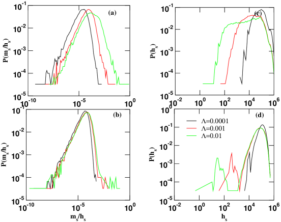
Figure 1: Distribution of the fields $m_{s}/h_{s}$ and of the fields $h_{s}$ for a the real degree distribution of the metabolic network of Saccharomyces cerevisiae (graphs (a) and (c))and for a graph with the same number of metabolites and reactions and the same number of nodes that the real metabolic network of Saccharomyces cerevisiae but with two delta peaks for the degree distribution (graphs (b) and (d)).

5 Conclusions

In this paper we have proposed a statistical mechanics approach for the study of flux-balance-analysis in a particular ensemble of metabolic networks. We have studied the impact of the topology of the networks on the distribution of the fluxes. We observe that the role of the real topological structure is to allow for larger variation of the fluxes, a fact that should have implications for the robustness of the system. In particular we found that the topology of real metabolites has an impact on the fat tail of the $m_{s}/h_{s}$ distribution and on the small $h$ field of the network, Further work is under consideration for the implementation of a message-passing algorithm able to predict the fluxes taking into account the full complexity of the real metabolic network.

6 Acknowledgments

We acknowledge E. Almaas, A. De Martino, R. Mulet and G. Semerjian for stimulating discussions.

References

- (1) R. Albert and A.-L. Barabási, Rev. Mod. Phys. 74, 47 (2002)
- (2) S. N. Dorogovtsev and J. F. F. Mendes, Evolution of Networks (Oxford University Press,Oxford,2003)
- (3) M. E. J. Newman, SIAM Rev. 45,167 (2003)
- (4) R. Pastor-Satorras and A. Vespignani, Evolution and Structure of the Internet (Cambridge University Press, Cambridge, 2004)
- (5) S. N. Dorogovtsev, A. V. Goltsev and J. F. F. Mendes arXiv:0705.0010 (2007)
- (6) S. N. Dorogovtsev, A. V. Goltsev and J. F. F. Mendes, Phys. Rev. E 66, 016104 (2002)
- (7) M. Leone, A. Vazquez, A. Vespignani and R. Zecchina, Eur. Phys. Jour. B 28, 191 (2002)
- (8) G. Bianconi, Phys. Lett. A 86, 5632 (2002)
- (9) R. Pastor-Satorras and A. Vespignani, Phys. Rev. Lett. 86, 3200 (2001)
- (10) A. E. Motter, C. Zhou, and J. Kurths Europhys. Lett. 69, 334 (2005)
- (11) Y. Moreno and A. F. Pacheco, Europhys. Lett. 68,603 (2004)
- (12) B. Kolman and R. Beck: Elementary linear programming with applications , 2nd edn (Academic Press, New York 1980)
- (13) Reconstructed metabolic networks of several model organisms can be found in the BIGG database at http://www.bigg.ucsd.edu.
- (14) H. Jeong, B. Tombor, R. Albert, Z. N. Oltvai, and A.-L. Barabasi, Nature 407, 651-654 (2000)
- (15) E. Ravasz, A. L. Somera, D. A. Mongru, Z. N. Oltvai and A. L. Barabási, Science 297,1551 (2002)
- (16) R. Tanaka, Phys. Rev. Lett. 94,168101 (2005)
- (17) J. S. Edwards and B. O. Palsson, PNAS 97 5528 (2000)
- (18) J. S., Edwards, R. U. Ibarra and B. O. Palsson, Nature Biotech.19, 125-130 (2001)
- (19) R. U., Ibarra, J. S. Edwards, and B. O. Palsson, Nature 420, 186-189 (2002)
- (20) D. Segre D. Vitkup and G. M. Church, PNAS 99 15112 (2002)
- (21) T Sholmi, O. Berkman and E. Ruppin, PNAS 24, 7695 (2005)
- (22) M. Emmerling et al. Journ. Bacteriology 184,152 (2002)
- (23) E. Almaas, B. Kovacs, T. Vicsek, Z.N. Oltvai and A.-L. Barab si Nature 427, 839-843 (2004)
- (24) F. Chung and L. Lu, PNAS 99, 15879 (2002)
- (25) G. Caldarelli, A. Capocci, P. De Los Rios and M. A. Muñoz Phys. Rev. Lett. 89, 258702 (2002)
- (26) K.-L. Goh, B. Kahng and D. Kim, Phys. Rev. Lett. 87 278701 (2001)
- (27) M. Molloy and B. Reed, Random Structures and Algorithms 6, 161 (1995)
- (28) G. Biroli and R. Monasson, J. Phys. A 32, L255 (1999)
- (29) G. Semerjian and L. F. Cugliandolo, Jour. Phys. A 35, 4837 (2002)
- (30) A. De Martino, C. Martelli, R. Monasson, I. Perez Castillo arXiv:cond-mat/0703343
- (31) R. Monasson, J. Phys. A 31,513 (1998).