Stability of the splay state in pulse–coupled networks

Abstract

The stability of the dynamical states characterized by a uniform firing rate (splay states) is analyzed in a network of globally coupled leaky integrate-and-fire neurons. This is done by reducing the set of differential equations to a map that is investigated in the limit of large network size. We show that the stability of the splay state depends crucially on the ratio between the pulse–width and the inter-spike interval. More precisely, the spectrum of Floquet exponents turns out to consist of three components: (i) one that coincides with the predictions of the mean-field analysis [Abbott-van Vreesvijk, 1993]; (ii) a component measuring the instability of “finite-frequency” modes; (iii) a number of “isolated” eigenvalues that are connected to the characteristics of the single pulse and may give rise to strong instabilities (the Floquet exponent being proportional to the network size). Finally, as a side result, we find that the splay state can be stable even for inhibitory coupling.

I Introduction

Understanding the mechanisms of information processing in the brain can be tackled by analyzing the dynamical properties of neural network models. Nonetheless, approaching the problem in full generality is a formidable task, since it requires taking into account, (i) the role of the topology of the connections, (ii) the dynamics of the connection themselves as a representation of the synaptic plasticity, (iii) the internal dynamics of the model neurons, which can depend on the number of ionic channels and other variables and parameters, (iv) the diversity among neurons and connections, (v) the unavoidable presence of noise. On the other hand, we can conjecture that at least some basic mechanisms are quite robust and may depend on a few ingredients, only. In fact, even simple models made of globally coupled identical units exhibit interesting dynamical properties, far from being completely interpreted. For instance, the stability of their steady states is still a debated problem. In fact, one can find claims that the splay state nicols , characterized by a uniform spiking rate of the neurons, is stable only in the presence of excitatory coupling abbott , and yet stable splay states have been found also in networks with fully inhibitory coupling zillmer . The standard approach for determining the stability properties of such simple models is based on the mean field approximation. This allows to obtain the spectrum of eigenvalues associated with the stability matrix in the thermodynamic limit $N\to\infty$, $N$ denoting the number of neurons. It is far from obvious if and how such results can be extended to the stability problem of large but finite networks. This is all more important if we consider that in the thermodynamic limit the splay state has been shown to be marginally stable for finite pulse–width, while it has been found to be strictly stable for $\delta$-like pulses Zumdieck-Timme:2004 ; zillmer . Moreover, we have discovered that in the limit of vanishing pulse–width, the formula derived in abbott does not coincide with the result of direct simulations.

We want to point out that assessing the linear stability of the splay state is just a preliminary step towards a complete undertanding of the dynamical properties of neural networks. Nonetheless, even the accomplishment of this “simple” task is going to reveal unexpected subtleties, which should be taken into account for pursuing further progresses. In particular, in this paper we introduce a specific formalism for determining the stability of the splay state in (in)finite ensembles of neurons. The approach is not entirely new, as it is based on the introduction of a Poincaré section, which transforms the original dynamical system into a map connecting dynamical configurations of the neural network after consecutive neural pulses (spikes) . A similar technique was used in Jin:2002 for obtaining analytic upper bounds of the maximum stability exponent of disordered neural networks with global inhibition. In bressloff such a technique was exploited to setup a general approach for the investigation of various dynamical regimes, including the splay state. The analysis was performed by considering the dynamical transformation describing consecutive spikes of the same neuron: due to its complicacy such a transformation does not allow to proceed much beyond formal statements. In this paper we have taken advantage from the idea of constructing a map between consecutive spikes of whatever neurons, combined with a suibtale shift of the neuron labels. In this way the computational complexity is significantly reduced with respect to bressloff and we are able to obtain analytic expressions also for large finite values of $N$.

One important consequence of our analysis is that one must be extremely careful when dealing with the stability problem genereated by finite pulse–width in large networks. Actually, even if the leading correction to the mean–field approximation is found to be ${\mathcal{O}}(1/N)$, we show that higher order corrections, up to ${\mathcal{O}}(1/N^{3})$ , have to be taken into account for determining the correct stability properties, even for arbitrarily large values of $N$.

Another important result of our study is that the thermodynamic limit does not commute with the zero pulse–width limit. In order to clarify this issue we consider the stability problem in the presence of pulses, whose width is inversely proportional to $N$. Although this recipe may appear a mathematical trick, it allows to point out a crucial aspect of the problem at hand: when both $N$ and the spiking rate are large, their ratio is the only relevant stability parameter. This implies also that the stability of a network subject to fixed small pulse-widths may qualitatively change when $N$ is increased, precisely because the above mentioned ratio varies.

In this paper we also clarify the basic question whether a given network of pulse–coupled neurons exhibits a finite stability or if it is “marginally” stable. A general formula obtained in abbott indicates that the amplitude of the eigenvalues of the stability spectrum of the splay state converges to zero from below as $1/N^{2}$. This implies that infinitely large networks exhibit an arbitrarily large number of eigenvalues arbitrarily close to zero. Accordingly, one should conclude that marginal stability is a generic feature of infinite networks. This seems to contrast with the result of Ref. zillmer , where numerical evidence of stability in the thermodynamic limit was found for $\delta$-like pulses. Our analysis clarifies that the Abbott-Van Vreeswijk’s formula abbott applies to the case of finite pulse–width, while in the case of vanishing pulse–width, stability is maintained also in the thermodynamic limit. The following argument provides a heuristic explanation of the mechanism generating such different stability conditions. In networks of pulse–coupled oscillators the same pulse acts differently on the various oscillators, because they can be located in different regions of their phase space, when the pulse is received. If the states of two neurons are close to each other in phase space (e.g., the neurons exhibit almost equal values of their membrane potentials), they will experience only slightly different effects from the same pulse of finite width. This amounts to say that the two neurons are very weakly coupled, thus yielding very small values of the Floquet stability exponent. The same is no longer true when very small (infinitesimal) pulse–widths are considered, since the coupling field strongly oscillates also over “microscopic” time scales, even for large values of $N$ . In other words, the “roughness” of the coupling is able to strongly lock the neurons, thereby yielding a finite stability of the splay state.

By this argument one can also understand the limitations of the mean-field approach proposed in abbott . In fact, once the neurons are ordered according to their instantaneous potential, we have verified that in many cases the stability of the state is controlled by the stability of “high-frequency” modes. A typical example of such a mode is the perturbations associated with the forward (backward) shift of the even (odd) neurons (see Section IV). These modes are by definition neglected in the mean–field approach abbott .

In Sec. II we describe the model of leaky integrate-and-fire neurons considered in this paper and we reduce it in full generality to an event-driven map. Moreover, also the formalism for the linear stability analysis is introduced. In Sec. III, we discuss the stability of the splay state in the case of finite pulse-width. Sec. IV is devoted to the analsysis of vanishing ($1/N$) pulse-widths. A brief summary of the results and future perspectives are reported in Sec. V.

II The model

We consider a simple model of a network of identical leaky integrate-and-fire neurons, whose interaction is mediated by a field $E(t)$ . This field can be viewed as the result of the linear superposition of single–neuron pulses $E_{s}(t)$, emitted when the membrane potential reaches a given threshold value. In agreement with Ref. abbott , we assume that the time dependence of a single pulse is given by the relation $E_{s}(t)=\alpha^{2}te^{-\alpha t}\,$, where $1/\alpha$ is the pulse–width. Accordingly, in between consecutive spikes, the field evolution is described by the differential equation,

$$\ddot{E}(t)+2\alpha\dot{E}(t)+\alpha^{2}E(t)=0\ .$$ (1)

Moreover, the effect of the pulse emitted at time $t_{0}$ amounts to a discontinuous change of the derivative,

$$\dot{E}(t_{0}^{+})=\dot{E}(t_{0}^{-})+\alpha^{2}/N\ .$$

The dynamics of the membrane potential $x_{i}(t)$ of the $i$–th neuron is determined by the differential equation

$$\dot{x}_{i}=a-\eta x_{i}+gE(t)\,,\ x_{i}\in(-\infty,1)\ ,\\$$ (2)

where the parameter $g$ gauges the strength of the coupling with the pulse field $E(t)$. The membrane potential evolves according to (2) until it reaches its threshold value $x_{i}=1\,$, when it is instantaneously reset to the value $x_{i}=0$ . Such a condition amounts to representing the discharge mechanism in neurons as a strong nonlinear effect associated with a discontinuity in the membrane potential. One should point out that this model is written from the very beginning in adimensional rescaled units (for a comparison with physical scales see the discussion in ref. zillmer  ) . Without prejudice of generality one can further simplify the equations by fixing the scale of time in units of the parameter $\eta^{-1}=1$. Consistently, one should formally rescale also the parameter $\alpha$ to $\alpha/\eta$.

II.1 Event-driven map

By integrating Eq. (1) between successive pulses, one can reduce the continous–time evolution of the interaction field $E(t)$ to the discrete map,

$$E(n+1)=E(n)e^{-\alpha\tau}+NQ(n)\tau e^{-\alpha\tau}$$ (3a)

$$Q(n+1)=Q(n)e^{-\alpha\tau}+\frac{\alpha^{2}}{N^{2}}\ ,$$ (3b)

where $\tau$ is the interspike time interval and we have introduced the new variable $Q:=(\alpha E+\dot{E})/N\,$ .

Accordingly, also the differential equations (2) can be integrated by taking into account this map-like representation of the field evolution and reduced to an event–driven map for the membrane potential $x_{i}\,$,

$$x_{i}(n+1)=x_{i}(n)e^{-\tau}+a\left(1-e^{-\tau}\right)+gF(n)\ \qquad i=1,\dots,N\enskip.$$ (4)

where $F$ is

$$F(n)=\frac{{\rm e}^{-\tau}-e^{-\alpha\tau}}{\alpha-1}\left(E(n)+\frac{NQ(n)}{\alpha-1}\right)-\frac{\tau e^{-\alpha\tau}}{(\alpha-1)}NQ(n)~{}.$$ (5)

If the integer $m$ labels of the closest–to–threshold neuron, the interspike time interval $\tau$ is obtained by imposing the condition, $x_{m}(n+1)=1\,$,

$$\tau(n)=\ln\left[\frac{x_{m}(n)-a}{1-gF(n)-a}\right]\ .$$ (6)

Since in networks of identical neurons the order of the potentials $x_{i}$ is preserved, it is convenient to introduce a comoving spatial index frame, $j(n+1)=j(n)-1\,$, where the next firing neuron is always labelled by $j(n)=1$ and reset to $j(n+1)=N\,$ after the firing event. Accordingly, the map for the membrane potentials transforms into

$$x_{j-1}(n+1)=x_{j}(n)e^{-\tau}+1-x_{1}(n)e^{-\tau}\ \qquad j=1,\dots,N-1\enskip,$$ (7)

with the boundary condition $x_{N}=0$. The set of Eqs. (3,6,7) defines a discrete-time mapping (notice that in the comoving frame the label $m$ in Eq. (6) is always set equal to 1) , that is fully equivalent to the original set of ordinary differential equations. Altogether, it turns out that a network of $N$ identical neurons is described by $N+1$ equations: Two of them account for the dynamics of $E(n)$, while the remaining $N-1$ equations describe the evolution of the neurons ($x_{N}$ is no longer a variable being, by definition, equal to 0). Accordingly we see that, at variance with Ref. bressloff   where no field dynamics was explicitely introduced, the model has a finite dimension.

In this framework, the periodic splay state reduces to a fixed point that satisfies the following conditions,

$$\tau(n)\equiv\frac{T}{N}\ ,$$ (8a)

$$E(n)\equiv\tilde{E}\,,\ Q(n)\equiv\tilde{Q}\ ,$$ (8b)

$$\tilde{x}_{j-1}=\tilde{x}_{j}e^{-T/N}+1-\tilde{x}_{1}e^{-T/N}\ ,$$ (8c)

where $T$ is the time elapsed between two consecutive spike emissions of the same neuron. A simple calculation yields,

$$\tilde{Q}=\frac{\alpha^{2}}{N^{2}}\left(1-e^{-\alpha T/N}\right)^{-1}\,,\ \tilde{E}=T\tilde{Q}\left(e^{\alpha T/N}-1\right)^{-1}\ .$$

The solution of Eq. (8c) involves a geometric series that, together with the boundary condition $\tilde{x}_{N}=0\,$, leads to a transcendental equation for the period $T\,$. Not surprisingly, the result turns out to be independent of the pulse–width $\alpha\,$. For simplicity, we report only the leading terms for $N\gg 1\,$,

$$\tilde{x}_{N-j}=\frac{aT+g}{T}\left(1-e^{-j\,T/N}\right)\ ,$$ (9a)

$$T=\ln\left[\frac{aT+g}{(a-1)T+g}\right]\ .$$ (9b)

By assuming that the uncoupled neurons are in the repetitive firing regime, i.e. by taking $a>1$, the period $T$ is well defined in the excitatory case ($g>0$) only for $g<1$ ($T\to 0$, when $g$ approaches 1), while in the inhibitory case ($g<0$), a meaningful solution exists for any coupling strength ($T\to\infty$ for $g\to-\infty$).

II.2 Linear stability

The main complication of the linear stability analysis stems from the implicit dependence of $\tau$ on the relevant variables (see Eq. (6), where $m=1$ in the comoving frame we have adopted). By linearizing Eq. (6), we obtain

$$\delta\tau(n)=\tau_{x}\delta x_{1}(n)+\tau_{E}\delta E(n)+\tau_{Q}\delta Q(n)\ ;$$

where $\tau_{x}:=\partial\tau/\partial x_{1}$ and analogous definitions hold for $\tau_{E}$ and $\tau_{Q}$. The linear stability of the splay state is thus determined by the dynamics of the perturbations $\delta x_{j}$, $\delta E$, and $\delta Q$. This is expressed by the following set of linear equations

$$\delta x_{j-1}(n+1)=e^{-T/N}[\delta x_{j}(n)-\delta x_{1}(n)]+e^{-T/N}(\tilde{x}_{1}-\tilde{x}_{j})\delta\tau(n)\,,$$ (10a)

$$\delta E(n+1)=e^{-\alpha T/N}\delta E(n)+Te^{-\alpha T/N}\delta Q(n)-\left(\alpha\tilde{E}-N\tilde{Q}e^{-\alpha T/N}\right)\delta\tau(n)\,,$$ (10b)

$$\delta Q(n+1)=e^{-\alpha T/N}\delta Q(n)-\alpha\tilde{Q}e^{-\alpha T/N}\delta\tau(n)\,,$$ (10c)

which have been linearized around the fixed point (8) . The boundary conditon $x_{N}\equiv 0\,$ imposed by the comoving frame yields $\delta x_{N}=0\,$. In practice, the stability problem is solved by computing the Floquet spectrum of multipliers $\{\mu_{k}\}\,$, $k=1,\ldots,N+1\,$ associated with the eigenvalue problem of the set of linear equations (10) . In general the explicit computation has to be performed numerically.

For the sake of clarity, it is first convenient to discuss the trivial case of vanishing interaction, i.e. $g=0\,$. After simple calculations the eigenvalues turn out to be $\mu_{k}=\exp(i\varphi_{k})$, where $\varphi_{k}=\frac{2\pi k}{N}$, $k=1,\ldots,N-1$, and $\mu_{N}=\mu_{N+1}=\exp(-\alpha T/N)\,$. The last two exponents concern the dynamics of the coupling field $E(t)$, whose decay is ruled by the time scale $\alpha^{-1}\,$.

As soon as the coupling is on, small amplitude fluctuations $\sim{\mathcal{O}}(g/N)$ affect the neuron dynamics and the spectrum of Floquet multipliers takes the general form

$$\mu_{k}=e^{i\varphi_{k}}e^{T(\lambda_{k}+i\omega_{k})/N}\,,\ \varphi_{k}=\frac{2\pi k}{N}\,,\ k=1,\ldots,N-1\,,$$ (11)

$$\mu_{N}=e^{T(\lambda_{N}+i\omega_{N})/N}\,,\ \mu_{N+1}=e^{T(\lambda_{N+1}+i\omega_{N+1})/N}\,.$$

where, $\lambda_{k}$ and $\omega_{k}$ are the real and imaginary parts of the Floquet exponents. As an example, in Fig. 1 we show the spectrum of the Floquet multipliers of the splay state for excitatory coupling ($g>0$)  and finite values of $N$ . The multipliers with $k=1,\ldots,N-1$ are very close to the unit circle, while the two isolated multipliers $\mu_{N}$ and $\mu_{N+1}$ lay very close to the real axis inside the unit circle. We want to point out that already for $g/N\approx{\mathcal{O}}(10^{-2})$ the multipliers of the coupled case can be viewed as small “perturbations” of the uncoupled one. This observation supports the perturbative approach that we are going to discuss in the following sections.

Before accomplishing this task, it remains to comment that the variable $\varphi_{k}$ plays the same role of the wavenumber in the linear stability analysis of spatially extended systems, so that we can say that $\lambda_{k}$ characterizes the stability of the $k$–th mode. In the following analysis it is convenient to distinguish between modes characterized by $\varphi_{k}\approx 0,\mod(2\pi)+{\mathcal{O}}(1/N)$, and the other modes. Actually they identify two spectral components, that require a different mathematical treatment. The first component corresponds to the condition $||\mu_{k}-1||\sim N^{-1}$ and is referred to as long wavelengths (LWs), while the second one corresponds to $||\mu_{k}-1||\sim{\mathcal{O}}(1)$ and is referred to as, short wavelengths (SWs).

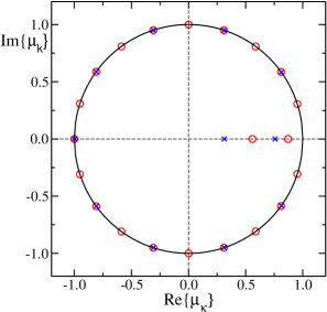
Figure 1: (Color online) Unitary circle and exact Floquet multipliers spectra for the complete maps for $N=20$ (red circles) and $N=10$ (blue crosses) for excitatory coupling. The parameters are $a=3.0$, $g=0.4$, and $\alpha=30.0$.

III Finite pulse–width

In this section we investigate the stability problem of the splay state for networks subject to pulses with finite $\alpha$ (i.e. independent of the system-size) for large values of $N$. This is also the setup studied in abbott by a mean field analysis. By retaining all the terms up to the order $1/N$, the event–driven map (see Eqs.(3) and (4) ) simplifies to the set of $N+1$ equations

$$E(n+1)=(1-\alpha\tau)E(n)+NQ(n)\tau\ ,$$ (12a)

$$Q(n+1)=(1-\alpha\tau)Q(n)+\frac{\alpha^{2}}{N^{2}}\ ,$$ (12b)

$$x_{j-1}(n+1)=(1-\tau)x_{j}(n)+1-x_{1}(n)+\tau\ ,$$ (12c)

where $j=1,\ldots,N-1$. Here the expression of interspike interval (6) simplifies to

$$\tau(n)=\frac{1-x_{1}(n)}{a-1+gE(n)}\ .$$ (13)

The periodic solution for the pulse–field becomes $\tilde{E}=T^{-1}\,$, and $\tilde{Q}=\alpha/NT\,$, while $\tilde{x}_{j}$ and the period $T$ are still given by Eq. (9). The Floquet eigenvalue spectrum $\mu_{k}\,$, $k=1,\ldots,N+1\,$, can be obtained by solving the set of $N+1$ linear equations

$$\mu_{k}\delta x_{j-1} = (1-T/N)\delta x_{j}-\delta x_{1}+(1-\tilde{x}_{j})\delta\tau\,,$$ (14a)

$$\mu_{k}\delta E = (1-\alpha T/N)\delta E+T\delta Q\,,$$ (14b)

$$\mu_{k}\delta Q = (1-\alpha T/N)\delta Q-\frac{\alpha^{2}}{NT}\delta\tau\,.$$ (14c)

An explicit expression for $\delta\tau$ is obtained by evaluating the derivatives of Eq. (13)

$$\delta\tau=-\frac{T^{2}}{N}\,\delta E-\frac{T}{g}\,\delta x_{1}\ .$$

With this substitution in Eqs.(14) we conclude that the eigenvalue problem amounts to finding the $N+1$ roots $\mu_{k}$ of the associated polynomial. A partial simplification of the problem can be obtained by extracting from Eqs.(14 b,c) the dependence of $\delta\tau$ directly in terms of the perturbation of the potential of the next–to–threshold neuron $\delta x_{1}$,

$$\delta\tau=K\delta x_{1}\,$$

where

$$K=\left[-(a-1+g/T)+\frac{\alpha^{2}gT}{N^{2}(\mu_{k}-1+\alpha T/N)^{2}}\right]^{-1}\,.$$ (15)

Finally, by substituting this expression into into Eq. (14a), we obtain a closed set of equations for the perturbations of the membrane potentials,

$$\mu_{k}\delta x_{j-1}=(1-T/N)\delta x_{j}+(K-1)\delta x_{1}-K\tilde{x}_{j}\delta x_{1}\ .$$ (16)

After imposing the boundary condition, $\delta x_{N}=0\,$, Eq. (16) reduces to the following eigenvalue equation,

$$\mu_{k}^{N-1}e^{T}=K(a+g/T)\frac{1-\mu_{k}^{N-1}}{1-\mu_{k}}-[K(a-1+g/T)+1]\frac{1-\mu_{k}^{N-1}e^{T}}{1-\mu_{k}e^{T/N}}\ ,$$ (17)

where $K$ is a function of $\mu_{k}\,$ (see Eq. (15)) .

In order to solve analytically the above equation, it is necessary to distinguish between long and short wavelengths.

III.1 Long wavelengths

Let us consider the modes for which $||\mu_{k}-1||\sim N^{-1}\,$, or, equivalently, $\varphi_{k}\approx 0,\mod(2\pi)+{\mathcal{O}}(1/N)$ . In order to simplify the notation we define

$$\Lambda_{k}:=\frac{N}{T}\ln\mu_{k}\,.$$

At leading order, $K$ writes

$$K=\left[-(a-1+g/T)+\frac{\alpha^{2}g}{T(\Lambda_{k}+\alpha)^{2}}\right]^{-1}\ .$$

Moreover, making use of the relation $\tilde{E}=T^{-1}$, the eigenvalue equation (17) can be approximated as

$$\frac{aT+g}{\alpha^{2}g}\left(1-e^{-\Lambda_{k}T}\right)(\Lambda_{k}+\alpha)^{2}(\Lambda_{k}+1)=\Lambda_{k}\left(e^{T}-e^{-\Lambda_{k}T}\right)\,,\ ||\Lambda_{k}||\neq 0\,.$$ (18)

This equation coincides with that one derived from the mean field analysis abbott , except for the missing $||\Lambda_{k}||=0\,$, which corresponds to the trivial zero Floquet exponent of the continuous time evolution (2) and disappears in the discrete-time dynamics. We want to stress again that, despite Eq. (18) yields $N+1$ roots, it provides a suitable approximation only for those eigenvalues which satisy the relation $||\mu_{k}-1||\sim N^{-1}\,$.

III.2 Short wavelengths

The second component of the spectrum (11) is obtained for $||\mu_{k}-1||\sim{\mathcal{O}}(1)$. In this case $K$ has the simple form

$$K=-(a-1+g/T)^{-1}\ .$$

Upon introducing into Eq. (17) the explicit form of the periodic solution (9b), the spectrum simplifies considerably, namely

$$\mu_{k}^{N}=e^{-T}\frac{a+g/T}{a-1+g/T}=1\ ,$$ (19)

i.e., it coincides with a fully degenerate Floquet spectrum,

$$\omega_{k}\equiv 0\,,\ \lambda_{k}\equiv 0\,$$ (20)

Notice that this approximation holds only for those eigenvalues such that $||\mu_{k}-1||\sim{\mathcal{O}}(1)$, i.e. those representing the large maiority of the spectrum, except those laying close to the point (1,0), where the unit circle intercepts the real axis (see Fig. 1)  .

For what concerns the isolated eigenvalues $\mu_{N}$ and $\mu_{N+1}$ one can easily argue that for finite $N$ and finite pulse–widths they are always contained inside the unit circle close to the real axis and they approch the point $(1,0)$ from the left as $N\to\infty$  . Accordingly, they can at most contribute to the marginal stability of the dynamics.

III.3 Phase diagram and finite-size corrections

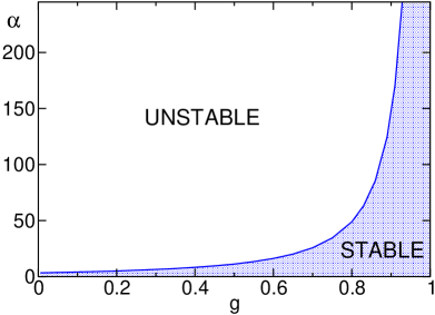
Figure 2: Phase diagram for the stability of the splay state in a neural network with excitatory coupling acting through finite pulse–width. The solid line separating the stable from the unstable regions in the $(g,\alpha)$-plane has been derived from the analytic formula of the Floquet spectrum (18) with $a=1.3\,$. Please notice that in this context stable refers to finite $N$, for infinite systems the stability will become marginal.

According to the above results one can conclude that in the limit $N\to\infty$ the onset of instabilities is determined by the Floquet exponents associated with LCs (see Eq. (18)). It is, therefore, not surprising to discover that our result coincides with the predictions of the mean–field analysis reported in abbott . We also confirm that the splay state is always unstable for inhibitory coupling ($g<0\,$). In the case of excitatory coupling the mean–field analysis predicts stability of the the splay state for $\alpha\leq\alpha_{c}(g,a)\,$, where the $\alpha_{c}(g,a)$ is the critical line separating the stable from the unstable region (see Fig. 2)) . By including the role of SWs we can conclude that in the limit $N\to\infty$ the splay state can be at most marginally stable for $\alpha\leq\alpha_{c}(g,a)\,$. In particular, $\alpha_{c}$ diverges to $+\infty$ for $g\to 1$ (see Fig. 2). Our analysis confirms also that the splay state becomes always unstable via a Hopf-bifurcation, that gives rise to collective periodic states vvres ; mohanty . For $g>1$ no splay state can exist and this can be viewed as a drawback of the model: for too strong excitatory coupling, no stationary regime can be sustained, since the evolution steadily accelerates.

The perfect degeneracy of the zero Floquet exponents associated to SWs sheds doubts on the effective stability properties of large but finite networks, since such modes turn out to be marginally stable. Therefore, we have decided to solve numerically the eigenvalue equations (10) for different system sizes and for values of the parameters $g$ and $\alpha$, which correspond to marginally stable splay states in the limit $N\to\infty$. The results plotted in Fig. 3) show that the splay state is strictly stable in finite lattices and that the maximum Floquet exponent approaches zero from below as $1/N^{2}$. This implies that a $1/N$ perturbation theory, like the one developed in this section, cannot account for such deviations and even a second-order approximation scheme cannot capture the instabilities of the original model. This is confirmed in Fig. 4, where the Floquet spectra obtained from first- and second-order approximations are seen to yield an unstable splay state, even though the numerical solution of the stability problem indicates that the finite–$N$ model is stable.

As the event-driven map is the standard approach adopted to simulate this type of networks, an important consequence of our analysis is that one should be careful enough to consider at least third order approximations in the $1/N$ perturbative expansion, otherwise the resulting approximate equations may fail to reproduce the correct asymptotic dynamics.

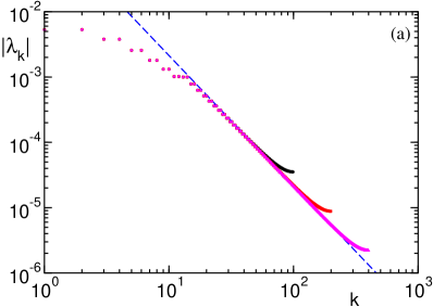
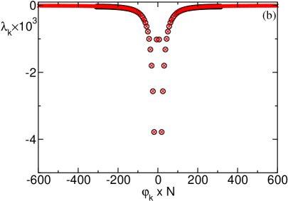
Figure 3: (Color online) (a) Log-log plot of the absolute values of the the Floquet exponents $\lambda_{k}$, ordered from the largest to the smallest as a function of the index $k=1,...,N$ for $N=100,200,400$. The dashed line has slope -2. (b) The Floquet exponent as a function of the rescaled phase $\varphi N$, for $N=100$ (black circles) and $N=200$ (red crosses). In both pictures the parameter values are $a=3.0$, $g=0.4$, and $\alpha=30.0$.

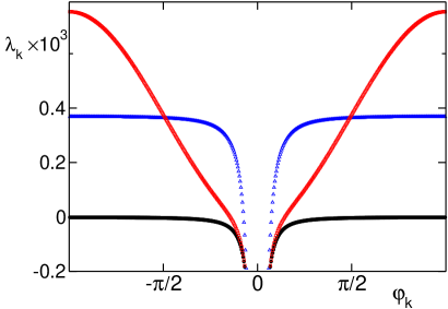
Figure 4: (Color online) Floquet exponents $\lambda_{k}(\varphi)$ as a function of the phase $\varphi_{k}$ for finite pulse–width $\alpha=3.0$ and finite neuron numbers $N=500$ in the case of excitatory coupling $g=0.4$. The filled circles represent the exact result for finite $N$, while the red empty squares and the blue empty triangles refer to approximated results correct up to the first or second order in $1/N$, respectively. The parameters here are $a=0.3$, $\eta=0.1$.

IV Vanishing pulse–width

In zillmer , we have investigated the synchronization properties of a network of leaky integrate-and-fire neurons in the case of $\delta$-like pulses. One might expect that the stability properties of such a network can be determined by taking the limit of vanishing pulse–width in the formulae obtained in Ref. abbott . However, the lack of agreement with numerics suggests that the $N\to\infty$ limit does not commute with the zero pulse–width limit. In order to clarify this issue, we introduce a new setup, where the pulse-width is rescaled with the network size $N$ as $N^{-1}\,$. This amounts to impose a decay rate proportional to $N$

$$\alpha:=\beta N.$$

It is important to notice that in this context we have to deal with two time scales: (i) a scale of order ${\mathcal{O}}(1)$ that corresponds to the evolution of the the membrane potential $x_{j}$; (ii) a scale of order $\alpha^{-1}\sim N^{-1}\,$ that corresponds to the field relaxation.

At leading order, the expression (5) for the auxiliary quantity $F(n)$ simplifies to

$$F(n)=\frac{1}{N\beta^{2}}\left[\beta E(n)\left(1-e^{-N\beta\tau}\right)+Q(n)\left(1-e^{-N\beta\tau}-N\beta\tau\,e^{-N\beta\tau}\right)\right]\ .$$

The splay state corresponds to the fixed–point

$$\tilde{Q}=\beta^{2}\left(1-e^{-\beta T}\right)^{-1}\,,\ \tilde{E}=T\tilde{Q}\left(e^{\beta T}-1\right)^{-1}\ ,$$

while the derivatives of the interspike interval (6) now read

$$\tau_{x}=\frac{N}{1-a-g\tilde{E}}\,,\ \tau_{E}=\frac{g}{N\beta}\left(1-e^{-\beta T}\right)\tau_{x}\,,\ \tau_{Q}=\frac{g}{N\beta^{2}}\left(1-e^{-\beta T}-\beta Te^{-\beta T}\right)\tau_{x}\ .$$

Finally, the eigenvalue spectrum is defined by the set of linear equations

$$\mu_{k}\delta x_{j-1} = (1-TN^{-1})\delta x_{j}-\delta x_{1}+N^{-1}(1-\tilde{x}_{j})\delta\tau\,,$$ (21a)

$$\mu_{k}\delta E = e^{-\beta T}\delta E+Te^{-\beta T}\delta Q-N\left(\beta\tilde{E}-\tilde{Q}e^{-\beta T}\right)\delta\tau\,,$$ (21b)

$$\mu_{k}\delta Q = e^{-\beta T}\delta Q-N\beta\tilde{Q}e^{-\beta T}\delta\tau\,.$$ (21c)

We repeat the same formal analysis illustrated in Sec. III, by first solving the eigenvalue equations for the field perturbations $\delta x_{j}$  . After some tedious calculations we obtain $\delta\tau=K\delta x_{1}\,$, where

$$K=\frac{(\mu_{k}e^{\beta T}-1)^{2}}{(\mu_{k}e^{\beta T}-1)^{2}(1-a-g\tilde{E})+\mu_{k}\beta^{2}Tg\,e^{\beta T}}\ .$$ (22)

By substituting this expression into Eq. (21) and by imposing the boundary condition $\delta x_{N}=0$, we obtain a closed equation for the spectrum $\{\mu_{k}\}\,$, $k=1,\ldots,N+1\,$,

$$\mu_{k}^{N-1}e^{T}=KC\frac{1-\mu_{k}^{N-1}}{1-\mu_{k}}-[K(C-1)+1]\frac{1-\mu_{k}^{N-1}e^{T}}{1-\mu_{k}e^{T/N}}\ ;$$ (23)

where $C:=(g+aT)/T\,$ and $K$ is still a function of $\mu_{k}$. Proceeding along the previous guidelines, it is necessary to separately discuss the behaviour of long and short wavelengths.

IV.1 Long wavelengths

As well as in Sec. III.1, we consider the spectral component characterized by $||\mu_{k}-1||\sim N^{-1}\,$. In this case $K$ assumes the simple expression

$$K=-\frac{1}{a-1}.$$

By neglecting $1/N$ terms, the spectrum satisfies the equation,

$$\left(1-e^{T\Lambda_{k}}\right)(1+\Lambda_{k}^{-1})=\left(1-e^{T(\Lambda_{k}+1)}\right)\frac{g}{aT+g}\ ,$$ (24)

where $\Lambda_{k}:=NT^{-1}\ln\mu_{k}\,$. This result agrees again with the mean field analysis abbott in the limit $\alpha\sim N\gg 1\,$. Let us remark that, despite Eq. (24) yields $N+1$ eigenvalues, it provides a good approximation only for those such that $||\mu_{k}-1||\sim N^{-1}\,$.

IV.2 Short wavelengths

For $||\mu_{k}-1||\sim{\mathcal{O}}(1)$ we can replace the term $(\mu_{k}e^{\beta T}-1)$ with $(e^{i\varphi_{k}+\beta T}-1)$, in Eq. (22), thus obtaining $K=K(\varphi_{k})\,$, for $k=1,\ldots,N-1\,$. Moreover, by using the expression (9b) for the period $T$, one can simplify Eq. (23) to the following form

$$\mu_{k}^{N}=e^{-T}(1-K)\,.$$ (25)

Accordingly, the Floquet spectrum writes

$$\lambda_{k}+i\omega_{k}=-1+\frac{1}{T}\ln[1-K(\varphi_{k})]-\frac{i\varphi_{k}N}{T}\,.$$ (26)

For even values of $N$ and for the maximal phase $\varphi_{1+N/2}=\pi\,$, an explicit solution for the Floquet exponent can be obtained:

$$\lambda_{\pi}:=\lambda_{1+N/2}=-1+\frac{1}{T}\ln\left[1+\frac{1}{a-1+2\beta^{2}Tg\left(1+e^{2\beta T}\right)\left(e^{3\beta T}-2e^{\beta T}+e^{-\beta T}\right)^{-1}}\right]\,.$$ (27)

IV.3 Isolated eigenvalues

The main consequence of the stability analysis discussed at the beginning of this section is that there exist also eigenvalues whose time scale is of the order $\alpha^{-1}\sim N^{-1}$. These exponents are those labelled with the indices $N$ and $N+1$ in Eq. (11). The analysis of these two exponents becomes particularly relevant when they approach and cross the unitary circle; their analytical expression can be easily derived by investigating the case $||\mu_{N,N+1}-1||\sim 1\,$, which leads to a divergence of the maximal Floquet exponent, $\lambda_{m}\sim N\,$. The two corresponding eigenvalues turn out to satisfy the equation

$$\frac{\lambda_{N,N+1}}{N}=-\beta+\frac{1}{T}\ln\left|1-\frac{\beta^{2}Tg}{2(1-a-g\tilde{E})}\left(1\pm\sqrt{1-\frac{4(1-a-g\tilde{E})}{\beta^{2}Tg}}\right)\right|$$ (28)

Whenever one of such solutions become positive, this will give a leading Floquet exponent $\lambda_{m}\sim N\,$.

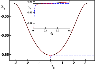
Figure 5: (Color online) Floquet spectrum $\lambda(\varphi)$ as a function of the phase $\varphi$ in the case of vanishing pulse–width. Red circles indicate the numerical results obtained for the linear stability analysis without any approximation for $N=1,000$, the black line refers to the first-order approximate expression (26) and the dashed blue line to the approximation (24). In the inset we magnify the region of small values of $\varphi$. The parameters are $a=1.3$, $g=-1.2$, and $\beta=1.0$.

IV.4 Phase diagram

The main difference with respect to the case of finite pulse–width is that the spectral component associated with SWs does not reduce to a fully degenerate zero Floquet exponent. On the contrary, it actively contributes to determining the stability properties of the network. While the splay state is found to be unstable for finite values of $\beta$ and excitatory coupling ($g>0$), a more interesting scenario is found for the inhibitory case ($g<0$)  .

Let us illustrate such situations by analyzing the stability spectrum obtained for $a=1.3$, $\beta=1.0$ and $g=-1.2$. In Fig. 5 we show that the theoretical expression (26) reproduces most of the spectrum obtained by the numerical diagonalization of the exact Jacobian for a network of 1000 neurons. In particular, the agreement is very good around the top part of the Floquet spectrum, which accounts for the stability of the network. More precisely, the least stable mode is that one characterized by the highest frequency (the $\pi$-mode), i.e. it corresponds to an up-down behavior of the perturbation, when passing from one to the next neuron. As this condition holds true for arbitrary values of $N$, we are led to conclude that one cannot perfom the continuum limit straightforwardly, since this would remove those fluctuations that are most relevant for the stability of the network.

Notice also that the only region where Eq. (26) fails to reproduce the true spectrum is close to vanishing values of the frequency $\varphi$. Analogously to the previous case, in this region (see the inset in Fig. 5) one has to invoke Eq. (24) to account for the dip centered around $\varphi\sim 0$.

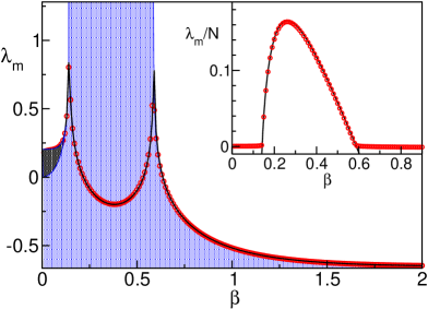
Figure 6: (Color online) Maximal Floquet exponent $\lambda_{m}$ as a function of $\beta$ for $a=1.3$ and $g=-1.2$. The line bordering the shaded region corresponds to the numerically obtained maximum in a network of $N=500$ neurons; red circles correspond to the second eigenvalue in the same network, while the solid line corresponds to the analytical expression (27) for $\lambda_{\pi}$. In particular, the lower border of the dark shaded region corresponds to $\lambda_{\pi}$. In the inset, the numerically computed Floquet exponent (open red circles) is compared to the analytical expression (28) for $\lambda_{N,N+1}$.

If one has to determine the entire spectrum of a finite network, the two components arising from Eqs. (24,26) have to be properly matched. After selecting equispaced modes according to the system size (the spacing being $2\pi/N$), one has to identify the value of $k$ where the distance between the two spectral components is minimal. Below this value the component to be considered is that of LWs (see Eq. (24)), while above such a value the spectrum is well approximated by Eq. (26)  .

It is also instructive to investigate the dependence of the spectrum on the parameter $\beta$. In Fig. 6 we have plotted the maximum Floquet exponent $\lambda_{m}$ as a function of $\beta$. The maximum has been determined by diagonalizing numerically the Jacobian for a network of $N=500$ neurons: it corresponds to the border of the shaded region (for the sake of clarity, the peak has been cut out). The comparison with the results obtained from Eq. (26) confirms that SW modes account for the stability of the entire network in a quite wide range of $\beta$ values, except for an intermediate region, where the maximum Floquet exponent is well reproduced by Eq. (28) (as it can be appreciated by looking at the inset of Fig. 6).

Outside this region, $\lambda_{m}$ is well reproduced by the analytical expression Eq. (27), except for $\beta<0.125$. Indeed, for small $\beta$, the maximum of the spectrum occurs for $|\varphi|<\pi$, as it can be seen in Fig. 7. Moreover, the maximal Floquet exponent $\lambda_{m}$ remains finite even for $\beta\to 0$. Finally, inside the intermediate region dominated by $\lambda_{N,N+1}$, the analytical prediction (27) is extremely close to the 2nd (numerically computed) exponent. Therefore, the theory exposed in this section predicts correctly the stability of the network, although one must carefully identify the spectral component that is responsible for the relevant contribution.

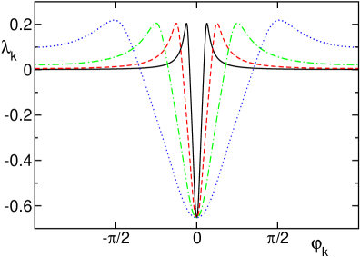
Figure 7: (Color online) Finite-frequency Floquet spectra $\lambda(\varphi)$ for $\beta=0.01$ (black solid line), 0.02 (red dashed line), 0.04 (green dot-dashed line) and 0.08 (blue dotted line) and $a=1.3$, $g=-1.2$.

There is another important conclusion that can be drawn from Fig. 6, by comparing two limit cases. On the one hand, the limit $\beta\to\infty$ corresponds to $\delta$-like pulse. In fact, one can see that the maximum Floquet exponent coincides with the expression derived in Ref. zillmer . On the other hand, for $\beta=0$, the model converges to the $\alpha\to\infty$ limit of the model considered in abbott . In the two limits,

$$\lambda_{\pi}=-\frac{g\beta^{2}T^{2}}{6[(a-1)T+g](aT+g)}$$ (29)

Altogether, the $\beta$-dependence resolves the contradiction mentioned in the beginning of this section, as we can conclude that the pulse–width does not only affect the quantitative value of the Floquet exponent, but contributes also to determining the qualitative stability properties. It is therefore useful to think about the meaning of $\beta$. It expresses the pulse bandwidth $1/\alpha$ in terms of “$1/N$” units. By remembering that the interspike interval is $T/N$, it is convenient to introduce the adimensional parameter

$$r=\frac{T/N}{1/\alpha}=\beta T\,.$$

This parameter, being the ratio between the interspike interval and the pulse–width, is susceptible of being determined in general contexts that go beyond the specific pulse-shape choice and model adopted in the present paper.

Actually, the phase diagram reported in Fig. 8, confirms that $r=\beta T$ is a meaningful parameter, since stable and unstable phases are separated by a critical line, where $r$ is constant independently of $g$. By solving $\lambda_{\pi}=0$, we find that the critical value of $r$ discriminating between stable and unstable phase is given by the following implicit equation

$${\rm e}^{4r}-2(r^{2}+1){\rm e}^{3r}-2r^{2}{\rm e}^{r}+1=0\quad.$$ (30)

Moreover, we see that the strongly unstable regime seen in Fig. 6 arises only for a sufficiently strong inhibitory coupling ($g<-1$).

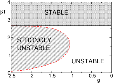
Figure 8: (color online) Phase diagram for the stability of the splay state for $a=1.3$ and inhibitory coupling in the sharp spike limit. The solid black horizontal line divides the stable from the unstable region, while the dashed red line encircle the strongly unstable phase where the maximum Floquet exponent is proportional to $N$.

We conclude this section by coming back to the possible reasons for the failure of the mean field approach. In the upper panel of Fig. 9, we show the time evolution of the field $E(t)$ for increasing values of $N$ and fixed $\alpha=120$. The oscillations around the mean value tend to decrease and this indeed suggests that it is meaningful to introduce a sort of average flux of spiking neurons as done in the mean field approach. One can also see that since $E(t)$ is increasingly flat (for increasing $N$), it is natural to expect that the stability of the splay state is very weak: The neuron-neuron interactions are in fact mediated by the common field $E$. It might be tempting to reduce the stability of the splay state to that of the single neuron exposed to a given field dynamics $E(t)$, but this would amount to no more than a crude approximation. In other words, there is no shortcut for performing the analysis carried out in this paper.

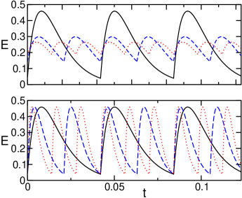
Figure 9: (Color online) Time evolution of the field $E(t)$ associated to a splay state for increasing $N$ values: $N=100$ (black solid lines), 200 (blue dashed lines), 300 (red dotted lines). The upper panel refers to a fixed value of $\alpha=120$, while the lower panel to a constant $\beta=0.14$. The other parameters are $a=1.3$ and $g=-1.2$

In the lower panel, of Fig. 9, the field evolution is reported for the same values of $N$ and $\beta=0.14$. In this case, field oscillations become faster but their size does not decrease upon increasing $N$. We consider this as the major reason for the failure of the mean field approach. Furthermore the finite amplitude of the oscillations is also responsible for mantaining a finite stability even in the limit $N\to\infty$  .

V Conclusions and perspectives

In this paper we have shown that the stability of splay states can be addressed by reducing a model of globally coupled differential equations to suitable event-driven maps which relate the internal configuration at two consecutive spike-emissions. The analytical investigation of the Jacobian in the large $N$ limit reveals that the spectrum of eigenvalues is made of three components: i) long wavelengths eigenmodes that emerge also from a mean-field approach abbott ; ii) short wavelengths; iii) isolated eigenvalues, which signal the existence of strong instabilities, i.e. eigenvalues that are proportional to the network size. Altogether, we find that drastically different results can be found for different values of the ratio $r$ between the interspike interval and the pulse–width. This leads us to conclude that the stability of large networks of neurons coupled via narrow pulses, crucially depends on the parameter $r$, thus suggesting that the dynamycal stability of these models demands a more refined treatment than mean–field. It will be interesting to investigate the role of $r$ in more general contexts, e.g., by considering different pulse shapes (possibly adding the effect of delay) and different force fields (possibly including further degrees of freedom, as it naturally appears in the Hodgkin-Huxley model).

Another issue that it will be worth analyzing concerns the exact stability in large but finite networks in the presence of finite pulse-widths. Our analysis has revealed that the first order approximations fails to reproduce even the sign of the maximum Floquet exponent. That is a consequence of the $1/N^{2}$ decay of the spectrum which, in turn, requires developing a third-order perturbation theory. Our numerics shows that the splay state is always stable towards SW perturbations in networks of LIF neurons with excitatory coupling, while a 1st and 2nd order approximation theories may give rise to unstable states. Is this an indication of a systematic drawback of discrete-time models, or an indication that qualitatively different stability properties may be found for different force fields? The analysis of nonlinear force fields is definitely needed for obtaining a convincing answer to this question.

References

- (1) S. Nichols and K. Wiesenfeld, Phys. Rev. A45, 8430 (1992); S.H. Strogatz and R.E. Mirollo, Phys. Rev. E47, 220 (1993).
- (2) L.F. Abbott and C. van Vreeswijk, Phys. Rev. E 48, 1483 (1993).
- (3) R. Zillmer, R. Livi, A. Politi, and A. Torcini, Phys. Rev. E 74 036203 (2006)
- (4) A. Zumdieck, M. Timme,T. Geisel, and F. Wolf, Phys. Rev. Lett. 93, 244103 (2004).
- (5) D. Z. Jin, Phys. Rev. Lett. 89, 208102 (2002).
- (6) P.C. Bressloff and S. Coombes, SIAM J. Appl. Math, 60, 820 (2000).
- (7) C. van Vreeswijk, Phys. Rev. E 54, 5522 (1996).
- (8) P.K. Mohanty and A. Politi, J. Phys. A:Math. Gen., 39, L415 (2006).