Results are presented on the discovery potential for MSSM neutral Higgs bosons in the $m_{\mathrm{h}}-{max}$ scenario. The region of large $\mathrm{tan\beta}$, between 15 and 50, and mass between $\approx$ 95 and 130 $\mathrm{Ge\kern-1.00006ptV}$  is considered in the framework of the ATLAS experiment at the Large Hadron Collider (LHC), for a centre-of-mass energy $\sqrt{s}$ = 14 TeV. This parameter region is not fully covered by the present data either from LEP or from Tevatron.

The h/A bosons, supposed to be very close in mass in that region, are studied in the channel h/A $\ra\mathrm{\mu^{+}\mu^{-}}$ accompanied by two b-jets. The study includes a method to control the most copious background, $\mathrm{Z}\ra\mathrm{\mu^{+}\mu^{-}}$ accompanied by two b-jets. A possible contribution of the H boson to the signal is also considered.

1 Introduction

The Minimal Supersymmetric Standard Model (MSSM) is the most investigated extension of the Standard Model (SM).

The theory requires two Higgs doublets giving origin to five Higgs bosons: two CP-even neutral scalars, h and H (h is the lighter of the two), one CP-odd neutral scalar, A, and one pair of charged Higgs bosons, $\mathrm{H^{\pm}}$  [1, 2, 3]. The discovery of any one of these particles is a crucial element for the confirmation of the model. This is a key point in the physics program of future accelerators and in particular of the LHC.

After the conclusion of the LEP program in the year 2000, the experimental limit on the mass of the Standard Model Higgs boson $\mathrm{H}$  was established at 114.4 GeV with 95% CL [4]. Limits were also set on the mass of neutral [5] and charged [6] MSSM Higgs bosons for most of the representative sets of model parameters.

The motivation of this study is to explore the potential of the ATLAS detector for the discovery of neutral MSSM Higgs bosons in the parameter region not excluded by the LEP and Tevatron data. We shall focus on the search for $\mathrm{h}$, the lightest of the neutral Higgs bosons. Its mass, taking account of radiative corrections, is predicted to be smaller than 140 $\mathrm{Ge\kern-1.00006ptV}$, see [5] and references therein. The search for a mass close to the mass of the Z boson, $m_{\mathrm{Z}}$, will be a challenging test of detector performance and of the analysis method of disentangling the signal from the background.

In the first part of this paper we review the MSSM framework, the production mechanism in hadron collisions, the present experimental situation and the discovery potential at the LHC.

In the second part, after describing the Monte Carlo generator and the software tools used, we discuss the detector performance relevant for this search of h, A and H, the analysis strategy and the results of the scan over the MSSM ($m_{\mathrm{A}}$, $\mathrm{tan\beta}$) plane. Details of this analysis are given in Ref. [7] and Ref. [8].

In the conclusion, results are presented on the neutral MSSM Higgs bosons discovery potential at the LHC based on the ATLAS detector.

2 Minimal Supersymmetric Standard Model

We discuss a few points of the model, useful for the present analysis. For a complete review see Refs. [9, 2]. At tree level, the masses of the five Higgs bosons of the MSSM are related by the following equations:

$$m_{H,h}^{2}=\frac{1}{2}[m_{A}^{2}+m_{Z}^{2}\pm\root \of{(m_{A}^{2}+m_{Z}^{2})^{2}-4m_{A}^{2}m_{Z}^{2}\cos^{2}2\beta}],$$ (1)

$$m_{H^{\pm}}^{2}=m_{\mathrm{W}}^{2}+m_{\mathrm{A}}^{2},$$

where $m_{\mathrm{W}}$ and $m_{\mathrm{Z}}$ are the W and Z masses, respectively, and $\mathrm{tan\beta}$ is the ratio of the vacuum expectation values of the two Higgs fields.

The MSSM model may be constrained by the assumption that the sfermions (scalar fermions) masses, the gaugino masses and the trilinear Higgs-fermion couplings must unify at the Grand Unification scale (GUT). In one of the possible constrained models the parameters chosen are:

• $M_{\mathrm{SUSY}}$, a common mass for all sfermions at the electroweak scale.

• $M_{\mathrm{2}}$, a common $\mathrm{S}U(2)_{L}$ gaugino mass at the electroweak scale.

• $\mu$, the strength of the supersymmetric Higgs mixing.

• $\mathrm{tan\beta}$, the ratio of the vacuum expectation values of the two Higgs fields .

• A = $\rm{A_{t}}$= $\rm{A_{b}}$ a common trilinear Higgs-squarks coupling at the electroweak scale. It is assumed to be the same for up-type squarks and for down-type squarks.

• $m_{\mathrm{A}}$, the mass of the CP-odd Higgs boson.

• $m_{\tilde{\mathrm{g}}}$, the gluino mass.

Three of these parameters define the stop and sbottom mixing parameters $\rm{X_{t}}=\rm{A_{t}}-\mu~{}\rm{cot}\beta$ and $\rm{X_{b}}=\rm{A_{b}}-\mu~{}\rm{cot}\beta$.

Whereas the particle spectrum depends on all the parameters mentioned above, the Higgs sector depends, at tree level, on only two parameters which can be taken to be $\mathrm{tan\beta}$ and $m_{\mathrm{A}}$, as in Eq. (1). The other parameters only enter through radiative corrections, but change the mass prediction of Eq. (1) (where it is limited to $m_{\mathrm{h}}<m_{\mathrm{Z}}$), allowing the mass of h to reach higher values ($\approx 130$ GeV in some scenarios, see Sec. 4.1).

Among all possible CP-conserving benchmark scenarios the so-called $m_{\mathrm{h}}-{max}$ scenario (Table 1) has been considered [5]. This scenario corresponds to the maximum value of the stop mixing parameter $\rm{X_{t}}$=A - $\mu~{}\rm{cot}\beta$ = 2$M_{\mathrm{SUSY}}$. Here the theoretical bound on the mass of the h is highest (hence the scenario’s name) and experimental limits are less constraining. Also, the range of excluded $\mathrm{tan\beta}$ values for given values of $m_{\mathrm{t}}$ (the top mass) and $M_{\mathrm{SUSY}}$ is the most conservative one.

Parameter	$m_{\mathrm{h}}-{max}$
$M_{\mathrm{SUSY}}$[$\mathrm{Ge\kern-1.00006ptV}$]	1000
$\mu$ [$\mathrm{Ge\kern-1.00006ptV}$]	-200
$M_{\mathrm{2}}$[$\mathrm{Ge\kern-1.00006ptV}$]	200
$\rm{X_{t}}$=A - $\mu~{}\rm{cot}\beta$	2$M_{\mathrm{SUSY}}$
$m_{\tilde{\mathrm{g}}}$[$\mathrm{Ge\kern-1.00006ptV}$]	0.8$M_{\mathrm{SUSY}}$
$m_{\mathrm{A}}$[$\mathrm{Ge\kern-1.00006ptV}$]	0.1-1000
$\mathrm{tan\beta}$	0.4-50

Table 1: CP-conserving benchmark $m_{\mathrm{h}}-{max}$ scenario .

We shall focus on the $m_{\mathrm{h}}-{max}$ scenario as the most promising for the search of the $\mathrm{h}$ boson, referring to it hereafter as MSSM.

At tree level the MSSM Higgs boson couplings to fermions and massive gauge bosons are obtained from the SM Higgs boson couplings via correction factors [10]. They depend on the parameters $\beta$ (already introduced) and $\alpha$, the mixing angle which diagonalizes the CP-even Higgs boson mass matrix. The two parameters are related by the following expression:

$$\cos 2\alpha=-\cos 2\beta\ \frac{m_{A}^{2}-m_{Z}^{2}}{m_{H}^{2}-m_{h}^{2}}$$ (2)

At high $\mathrm{tan\beta}$ the MSSM correction factors to the SM Higgs bosons couplings to fermions and massive gauge bosons are larger for down-type quarks (b) and leptons ($\tau$ and $\mu$) than for up type-quarks. Thus, the associated $\mathrm{b\bar{b}}$h production is enhanced and becomes the dominant process in the production of h bosons in the high $\mathrm{tan\beta}$ region.

The Feynman diagrams contributing to the process $\mathrm{gg}$$\to$ $\mathrm{b\bar{b}}\mathrm{h}\rightarrow\mathrm{\mathrm{b\bar{b}}\mathrm{\mu^{+}\mu^{-}}}$and $\mathrm{q\bar{q}}$$\to$ $\mathrm{b\bar{b}}\mathrm{h}\rightarrow\mathrm{\mathrm{b\bar{b}}\mathrm{\mu^{+}\mu^{-}}}$ are shown in Fig. 1.

Figure 1: Typical diagrams contributing at “tree level” to the process $\mathrm{gg}$$\to$ $\mathrm{b\bar{b}}\mathrm{h}\rightarrow\mathrm{\mathrm{b\bar{b}}\mathrm{\mu^{+}\mu^{-}}}$and $\mathrm{q\bar{q}}$$\to$ $\mathrm{b\bar{b}}\mathrm{h}\rightarrow\mathrm{\mathrm{b\bar{b}}\mathrm{\mu^{+}\mu^{-}}}$.

We shall consider mainly the decays to $\mathrm{\mu^{+}\mu^{-}}$. Indeed, although the Higgs boson couplings are proportional to the fermion mass, thus resulting in a branching ratio to $\mathrm{\tau^{+}\tau^{-}}$ higher than to $\mathrm{\mu^{+}\mu^{-}}$  by a factor $(\frac{m_{\tau}}{m_{\mu}})^{2}$, the experimental conditions favor the $\mathrm{\mu^{+}\mu^{-}}$ channel.

In the region of high $\mathrm{tan\beta}$  and $m_{\mathrm{h}}\approx 100$ $\mathrm{Ge\kern-1.00006ptV}$ the CP-odd neutral Higgs boson A has a mass only slightly higher than the CP-even h and a competitive branching ratio for the $\mathrm{\mu^{+}\mu^{-}}$ decay channel [10]. Also, cross-sections and widths, which are functions of the parameters $\mathrm{tan\beta}$  and $m_{\mathrm{A}}$, are close in some regions of the parameter space (Sec. 4.1 ). Thus, in these regions the h and A bosons are indistinguishable from an experimental point of view, and it is more correct to think in terms of a h/A search. In the following we refer to the boson sought as the h/A boson (however its mass is noted $m_{\mathrm{h}}$ or $m_{\mathrm{A}}$, accordingly) . The degeneracy between h and A is less pronounced near the higher mass limit of h .

3 Experimental search for Minimal Supersymmetric Standard Model Higgs

3.1 LEP and Tevatron results

High precision tests of the Standard Model have been performed at LEP setting a combined limit of $m_{\mathrm{H}}$$>$ 114.4 $\mathrm{Ge\kern-1.00006ptV}$ for the mass of the SM Higgs boson [4].

Again at LEP, the validity of the Minimal Supersymmetric Standard Model has been investigated within the constrained framework of Sec. 2. For the mass of the charged MSSM Higgs bosons a combined limit $m_{\mathrm{H_{\pm}}}$$>$ 78.6 $\mathrm{Ge\kern-1.00006ptV}$ was obtained [6]. Searching for neutral CP-even and CP-odd MSSM Higgs bosons, no indication of signal was found up to a center-of-mass energy of 209 $\mathrm{Ge\kern-1.00006ptV}$ [5]. The corresponding lower limits on the masses were set as a function of $\mathrm{tan\beta}$ for several scenarios. In the $m_{\mathrm{h}}$-max scenario (Fig. 2) with a top mass $m_{\mathrm{t}}$=174.3 $\mathrm{Ge\kern-1.00006ptV}$  the limits for $\mathrm{tan\beta}>10$ at 95% CL are approximately :

$$m_{\mathrm{h}},m_{\mathrm{A}}\geq 93~{}\mathrm{Ge\kern-1.00006ptV}$$

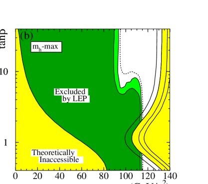
Figure 2: The combined LEP results for the search for the MSSM neutral Higgs bosons (from Ref. [5]). The figure shows the theoretically inaccessible regions (light-grey/yellow) and the regions experimentally excluded by LEP searches, at 95% C.L. (medium-grey/light-green) and 99.7% C.L. (dark-grey/dark-green), for the $m_{\mathrm{h}}$-max scenario with the top mass $m_{\mathrm{t}}$= 174.3 $\mathrm{Ge\kern-1.00006ptV}$, in two projections of the MSSM parameters ($m_{\mathrm{h}}$, $m_{\mathrm{A}}$), ($m_{\mathrm{h}}$, $\mathrm{tan\beta}$). The dashed lines indicate the boundaries of the regions which are expected to be excluded, at 95% C.L., on the basis of Monte Carlo simulations with no signal. In the ($m_{\mathrm{h}}$, $\mathrm{tan\beta}$) projection, the upper boundary of the parameter space is indicated for four values of the top mass; from left to right: $m_{\mathrm{t}}$= 169.3, 174.3, 179.3 and 183.0 $\mathrm{Ge\kern-1.00006ptV}$.

A complementary search, providing sensitivity in the region $\mathrm{tan\beta}>50$ has been performed at the Tevatron Collider at $\sqrt{s}$= 1.96 $\mathrm{Te\kern-1.00006ptV}$. In the MSSM scenario, a significant portion of the parameter space has been excluded by the D0 Collaboration, down to $\mathrm{tan\beta}$ = 50 as a function of $m_{\mathrm{A}}$, by studying the associated production with two b quarks of h/A/H bosons and their decay into $\mathrm{b\bar{b}}$ [11]. Comparable results have been obtained by the CDF Collaboration exploring the h/A/H decays to $\mathrm{\tau^{+}\tau^{-}}$, but extending the excluded region to higher values of $m_{\mathrm{A}}$ [12].

3.2 LHC discovery perspectives

The LEP and Tevatron data don’t exclude the parameter space defined by $\mathrm{tan\beta}$ larger than 10 and smaller than 50. Therefore, a natural continuation of the LEP and Tevatron physics is the investigation of the possible existence of MSSM Higgs bosons in this region of $\mathrm{tan\beta}$. The ATLAS [13] and CMS [14] experiments starting in the near future at the Large Hadron Collider (LHC), at CERN, constitute an excellent laboratory for such search.

The prospect for the detection of MSSM Higgs bosons at LHC was evaluated for benchmark sets preventing Higgs boson decays to SUSY particles [10, 13] and focusing on the discovery potential of decay modes common to MSSM and SM Higgs bosons [13]. It was concluded that the complete region of parameter space $m_{\mathrm{A}}$ = 50 – 500 $\mathrm{Ge\kern-1.00006ptV}$ and $\mathrm{tan\beta}$  = 1 – 50 is open to Higgs boson discovery by the ATLAS experiment, already with an integrated luminosity of $\int\!{\cal L}\,\mathrm{d}t$ = 30 $\mathrm{fb^{-1}}$, and that over a large part of this region more than one Higgs boson and more than one decay mode could be observed – the detection of a signal in more than one decay channel would constitute strong evidence for the MSSM model. It was also found that the region in the ($m_{\mathrm{A}}$, $\mathrm{tan\beta}$) plane which corresponds to $m_{\mathrm{h}}$ $\approx$ 100 $\mathrm{Ge\kern-1.00006ptV}$ and $\mathrm{tan\beta}\ >10$ is only accessible by a neutral h/A boson decaying to $\mathrm{\mu^{+}\mu^{-}}$ or $\mathrm{\tau^{+}\tau^{-}}$ [10, 13], and by a charged $\mathrm{H^{\pm}}$ boson decaying to $\tau\nu$ [15].

More recently the h boson discovery potential in the MSSM scenario has been investigated [16] at two luminosities, $\int\!{\cal L}\,\mathrm{d}t$= 30 $\mathrm{fb^{-1}}$ and $\int\!{\cal L}\,\mathrm{d}t$= 300 $\mathrm{fb^{-1}}$ . At low luminosity the $\mathrm{h}\ra\mathrm{\tau^{+}\tau^{-}}$ decay mode represents the main contribution to the discovery potential and covers most of the parameter space not yet explored. However the contribution of $\mathrm{b\bar{b}}$$\mathrm{h}\ra\mathrm{\mu^{+}\mu^{-}}$ appears to be crucial in the region of moderate $\mathrm{tan\beta}$ and mass close to $m_{\mathrm{Z}}$. The channel $\mathrm{b\bar{b}}\mathrm{h}\ra\mathrm{\mu^{+}\mu^{-}}$ which requires an excellent performance in $\mu$ detection and b-tagging is well suited to the ATLAS experiment thanks to a design giving high performance from the muon spectrometer and the inner detector.

At high luminosity channels such as: $\mathrm{h}\ra\gamma\gamma$, $\mathrm{h}\ra\mathrm{Z}\mathrm{Z}\ra 4\ell$ and $\mathrm{h}\ra\mathrm{b\bar{b}}$ in associated production with $\mathrm{t\bar{t}}$  give a significant contribution. The channel $\mathrm{h}\ra\gamma\gamma$, which requires an excellent $M_{\gamma\gamma}$ mass resolution and jet/$\gamma$ separation, corresponds to MSSM rates suppressed with respect to the SM case but for a limited region of the parameter space where they could even be slightly enhanced. As for the channel $\mathrm{h}\ra\mathrm{b\bar{b}}$, only the $\mathrm{t\bar{t}}$h production followed by the $\mathrm{h}\ra\mathrm{b\bar{b}}$ decay can be observed clearly above the background, thus the extraction of the signal requires the identification of four b-jets and an excellent b-tagging performance. In the MSSM case the rates could be enhanced by 10-20% over the SM rates.

3.3 Background processes

The prospects for the detection of MSSM Higgs bosons at LHC depend heavily on the suppression of the background sources:

• $\mathrm{Z}/\gamma^{*}$ production with two b-jets and a subsequent decay into a $\mathrm{\mu^{+}\mu^{-}}$ pair. The cross section for this process is a few orders of magnitude larger than for the signal. As an example, we quote for the $\mathrm{Z}$ boson $\sigma_{\mathrm{b\bar{b}}\mathrm{Z}}\cdot\rm{Br_{\mathrm{Z}\ra\mathrm{\mu^{+}\mu^{-}}}}\approx$ 22.8 $\mathrm{pb}$  and for each of the h and A bosons $\sigma_{\mathrm{h}/\mathrm{A}\mathrm{b\bar{b}}}\cdot\rm{Br}_{\mathrm{h}/\mathrm{A}\ra\mathrm{\mu^{+}\mu^{-}}}\approx\ 0.24$ $\mathrm{pb}$ (at $\mathrm{tan\beta}$ = 45 and $m_{\mathrm{h}}$ = 110 $\mathrm{Ge\kern-1.00006ptV}$).

  

  

  Figure 3: Typical diagrams contributing at “tree level” to the process $\mathrm{gg}$$\to\mathrm{Z}/\gamma^{*}\mathrm{b\bar{b}}\to\mathrm{\mu^{+}\mu^{-}}\mathrm{b\bar{b}}$ and $\mathrm{q\bar{q}}~{}\to~{}\mathrm{Z}/\gamma^{*}\mathrm{b\bar{b}}~{}\to~{}\mathrm{\mu^{+}\mu^{-}}\mathrm{b\bar{b}}$.

  The corresponding diagrams are shown in Fig. 3 and Fig. 1, respectively. It is clear that they differ only in the kind of boson produced, h (or A) in the signal and $\mathrm{Z}/\gamma^{*}$ in the background. The distinction between the signal and the background when $m_{\mathrm{h}}$ is approaching $m_{\mathrm{Z}}$ becomes then an extremely hard task due to the similar topology of the decays [7], although angular distributions differ somewhat due to the fact the boson is a scalar in one case and a vector in the other.

• $\mathrm{Z}$  production with two jets not originating from b-quarks. The cross section is $\approx 24$ times that for Z with two b-jets and can contribute to the background in case of jet misidentification. An estimate of a possible impact on the significance of this analysis is reported in Sec. 7.2.

• $\mathrm{Z}$$\mathrm{Z}$ associated production, when one $\mathrm{Z}$ decays into $\mathrm{b\bar{b}}$ and the second one decays into $\mathrm{\mu^{+}\mu^{-}}$. This process has a cross section of the same order of magnitude as the signal, $\sigma_{\mathrm{Z}\mathrm{Z}}\cdot\rm{Br_{\mathrm{Z}\ra\mathrm{\mu^{+}\mu^{-}}}}\cdot\rm{Br_{\mathrm{Z}\ra\mathrm{b\bar{b}}}}\approx\ 0.13~{}\mathrm{pb}$ , but can be easily suppressed using the kinematic characteristics of the events, see following sections.

• $\mathrm{t\bar{t}}$ associated production followed by a top-quark decay into a b-quark and a W boson and a subsequent W decay in $\mu\nu$. The cross section of this process is $\sigma_{\mathrm{t\bar{t}}}\cdot{\rm Br_{t\ra b\W}}\cdot{\rm Br_{W\ra\mu\nu}}\cdot{\rm Br_{t\ra b\W}}\cdot{\rm Br_{W\ra\mu\nu}}\approx\ 5.71~{}\mathrm{pb}$ . The presence of two neutrinos implies missing transverse energy in the event (see following sections) thus allowing this background to be strongly reduced. One would want to discriminate the signal from the background on the basis of the different b-jets characteristics (the two background b-jets are usually more energetic than those accompanying the signal and the probability of their identification is higher), but the requirement that the two b-jets be identified will suppress the signal more than the background.

4 Monte Carlo simulation

We improve on the analyses reported in Sec. 3.2 with a full Monte Carlo simulation of the experiment (data generation, reconstruction and analysis). The exploration of the unexcluded MSSM parameter space, with a view to either discovering a supersymmetric Higgs boson or excluding the model considered, constitutes the motivation of the analysis described in this paper.

The considerations of Sec. 2 and Sec. 3 suggested a search for $\mathrm{h}/\mathrm{A}\ra\mathrm{\mu^{+}\mu^{-}}$ decays accompanied by two b-jets. The extraction of the h/A boson signal from the competing enormous background of Z decays in the mass region close to $m_{\mathrm{Z}}$ constitutes a challenging search, where all performances of the experimental setup have to be exploited.

To this purpose we have generated signal and background Monte Carlo events using the PYTHIA program (v.6.226) [18] as specified below, for a center-of-mass energy $\sqrt{s}$= 14 $\mathrm{Te\kern-1.00006ptV}$. The efficiency of the selection criteria, the detector acceptance and the purity of the data sample are estimated from these events and the ATLAS detector response [13]. The latter is simulated using the GEANT program [20, 21] which takes into account the effects of energy loss, multiple scattering and showering in the detector through an interface called ATHENA (v.10.0.1).

The number of events used in this analysis corresponds to an integrated luminosity $\int\!{\cal L}\,\mathrm{d}t=300~{}\mathrm{fb^{-1}}$ with the exception of the channel $\mathrm{b\bar{b}}\mathrm{Z}\rightarrow\mathrm{\mathrm{b\bar{b}}\mathrm{\mu^{+}\mu^{-}}}$. In this latter case, for practical reasons, a number of events corresponding to half the mentioned luminosity has been generated. We note that $\int\!{\cal L}\,\mathrm{d}t=300~{}\mathrm{fb^{-1}}$ corresponds to the integrated luminosity expected after three years of data taking.

4.1 Signal

The MSSM neutral Higgs bosons h, A and H were generated in associated production with two b-quarks using the PYTHIA program (v.6.226) through the ATHENA interface (v.9.0.4). The parameters of the model were given the values [22] shown in Table 2 (for $\mathrm{tan\beta}$ and $m_{\mathrm{A}}$ the range of values scanned is shown). In this parameter region, as mentioned in Sec. 2, the cross section, mass and width of h and A bosons are close while the H cross section is one order of magnitude lower than the h/A cross section.

As is done in the Pythia code, we have taken $m_{\mathrm{A}}$ as input parameter. The values of $m_{\mathrm{h}}$ and $m_{\mathrm{H}}$ are then derived from PYTHIA as a function of $m_{\mathrm{A}}$.

Parameter		value
common gaugino mass	$M_{\mathrm{2}}$$\equiv m_{1/2}$ [$\mathrm{Ge\kern-1.00006ptV}$]	200
gluino mass	$m_{\tilde{\mathrm{g}}}$ [$\mathrm{Ge\kern-1.00006ptV}$]	800
strength of supersymmetric Higgs	$\mu$ [$\mathrm{Ge\kern-1.00006ptV}$]	- 200
ratio of Higgs fields	$\mathrm{tan\beta}$	15-50
common scalar mass	$m_{0}$ [$\mathrm{Ge\kern-1.00006ptV}$]	1000
squark left 3 gen	$M_{\tilde{\rm qL}}$ [$\mathrm{Ge\kern-1.00006ptV}$]	1000
sbottom mass	$M_{\tilde{\rm bR}}$ [$\mathrm{Ge\kern-1.00006ptV}$]	1000
stop mass	$M_{\tilde{\rm tR}}$ [$\mathrm{Ge\kern-1.00006ptV}$]	1000
stop-trilinear coupling	A	2440
mass of CP-odd boson	$m_{\mathrm{A}}$  [$\mathrm{Ge\kern-1.00006ptV}$]	95-135

Table 2: Parameters for A, h and H generation in PYTHIA (v.6.226) [18].

The signal $\mathrm{b\bar{b}}\mathrm{h}\rightarrow\mathrm{\mathrm{b\bar{b}}\mathrm{\mu^{+}\mu^{-}}}$ has been simulated in 104 points of the parameter space ($m_{\mathrm{A}}$, $\mathrm{tan\beta}$), corresponding to eight steps in $\mathrm{tan\beta}$, chosen equally spaced between 15 and 50 and thirteen steps of 2.5 $\mathrm{Ge\kern-1.00006ptV}$  in $m_{\mathrm{h}}$  between 95 $\mathrm{Ge\kern-1.00006ptV}$ and 125 $\mathrm{Ge\kern-1.00006ptV}$ (the largest value allowed by PYTHIA (v.6.226)). These are also the points where the decay $\mathrm{b\bar{b}}\mathrm{A}\rightarrow\mathrm{\mathrm{b\bar{b}}\mathrm{\mu^{+}\mu^{-}}}$ has been simulated.

The values of the mass, cross section and width of the A/h and H neutral bosons are reported in Ref. [7] for all the points analyzed of the ($m_{\mathrm{A}}$, $\mathrm{tan\beta}$) plane. For the following discussion a reference point has been chosen at $\mathrm{tan\beta}$ = 45, $m_{\mathrm{A}}$=110.31  $\mathrm{Ge\kern-1.00006ptV}$ ($m_{\mathrm{h}}$= 110 $\mathrm{Ge\kern-1.00006ptV}$, $m_{\mathrm{H}}$= 127.46 $\mathrm{Ge\kern-1.00006ptV}$). The corresponding width is $\Gamma_{\mathrm{A}}$= 4.28 $\mathrm{Ge\kern-1.00006ptV}$ ($\Gamma_{\mathrm{h}}$= 4.20 $\mathrm{Ge\kern-1.00006ptV}$, $\Gamma_{\mathrm{H}}$= 0.05 $\mathrm{Ge\kern-1.00006ptV}$), while the production cross section times the branching ratio for the decay to $\mathrm{\mu^{+}\mu^{-}}$ is $\sigma_{\mathrm{b\bar{b}}\mathrm{A}\rightarrow\mathrm{\mathrm{b\bar{b}}\mathrm{\mu^{+}\mu^{-}}}}=0.243$ pb ($\sigma_{\mathrm{b\bar{b}}\mathrm{h}\rightarrow\mathrm{\mathrm{b\bar{b}}\mathrm{\mu^{+}\mu^{-}}}}=0.245$ pb, $\sigma_{\mathrm{b\bar{b}}\mathrm{A}\rightarrow\mathrm{\mathrm{b\bar{b}}\mathrm{\mu^{+}\mu^{-}}}}=0.0016$ pb).

4.2 Background

For convenience we list again below the sources of background considered in Sec. 3.3 which were fully simulated. The Z production associated with two jets not originating from b as yet has not been implemented in the AcerMC2.3 code and has been ignored at this level (see however end of Sec. 7.2).

• $\mathrm{b\bar{b}}\mathrm{Z}\rightarrow\mathrm{\mathrm{b\bar{b}}\mathrm{\mu^{+}\mu^{-}}}$. The events are generated by AcerMC(2.3) [17] with the hadronization process of PYTHIA (v.6.226) . At the generator level a cut-off is applied to the $\mathrm{\mu^{+}\mu^{-}}$ invariant mass, $M^{\mathrm{inv}}_{\mu\mu}>60~{}\mathrm{Ge\kern-1.00006ptV}$ .

• $\mathrm{t\bar{t}}\rightarrow\mathrm{\mathrm{b\bar{b}}\mathrm{\mu^{+}\mu^{-}}\mathrm{\nu\bar{\nu}}}$. The events are fully generated with PYTHIA (v.6.226).

• $\mathrm{Z}\mathrm{Z}\rightarrow\mathrm{\mathrm{b\bar{b}}\mathrm{\mu^{+}\mu^{-}}}$. The events are fully generated with PYTHIA (v.6.226).

process	$\sigma_{\mathrm{b\bar{b}}\mathrm{\mu^{+}\mu^{-}}}$	$\rm N^{\rm exp_{300}}$	$\rm N^{\rm MC}$	${\rm w}$
(background)	[pb]
$\mathrm{b\bar{b}}\mathrm{Z}\rightarrow\mathrm{\mathrm{b\bar{b}}\mathrm{\mu^{+}\mu^{-}}}$	22.789	6836700	3314000	2.06
$\mathrm{t\bar{t}}\rightarrow\mathrm{\mathrm{b\bar{b}}\mathrm{\mu^{+}\mu^{-}}\mathrm{\nu\bar{\nu}}}$	5.71	1713420	1806437	0.95
$\mathrm{Z}\mathrm{Z}\rightarrow\mathrm{\mathrm{b\bar{b}}\mathrm{\mu^{+}\mu^{-}}}$	0.1273	33819	97244	0.35

Table 3: Background cross section times branching ratios, $\sigma_{\mathrm{b\bar{b}}\mathrm{\mu^{+}\mu^{-}}}$, number of expected events for $\int\!{\cal L}\,\mathrm{d}t=300~{}\mathrm{fb^{-1}}$, $\rm N^{\rm exp_{300}}$, number of Monte Carlo generated events, $\rm N^{\rm MC}$, and their weight in the analysis, w, for the three processes considered.

The cross section times branching ratios, together with the number of expected events for $\int\!{\cal L}\,\mathrm{d}t=300~{}\mathrm{fb^{-1}}$, the number of Monte Carlo generated events and their weight, is reported in Table 3 for the three background processes.

Among these the main contribution comes from $\mathrm{b\bar{b}}\mathrm{Z}\rightarrow\mathrm{\mathrm{b\bar{b}}\mathrm{\mu^{+}\mu^{-}}}$, and is affected by a cross section uncertainty arising from uncertainties on QCD, QED couplings ($\approx 10\%$ [17]) and from higher order corrections ($\approx 25\%$ [23]). As we intend to account for this large uncertainty with a data-driven method (Sec. 6.3), a sample of $\mathrm{b\bar{b}}\mathrm{Z}\ra\ee$ events, $\approx$ 600000 events, corresponding to an integrated luminosity $\int\!{\cal L}\,\mathrm{d}t=30~{}\mathrm{fb^{-1}}$ with a cross section $\sigma\approx 22.8~{}\mathrm{pb}$, has also been simulated. Owing to the large number of events simulated, there is only a minor statistical uncertainty associated with the evaluation of the tails of $\mathrm{Z}\ra\mathrm{\mu^{+}\mu^{-}}$ background.

5 The ATLAS detector

Here we shall summarize the main features of the ATLAS detector  [24] which are relevant for the present analysis. For a more detailed information we refer to [25] :

• Magnet System: This consists of a solenoid providing a 2 T$\cdot$m bending power in the inner detector, and a barrel air toroid completed by two end-cap toroids, with a typical bending power of 6 T$\cdot$m and 3 T$\cdot$m respectively.

• Inner Tracking System: It has been designed to measure as precisely as possible and with high efficiency the charged particles emerging from primary interactions in a pseudorapidity range $\left|\eta\right|<2.5$. It is installed inside in the solenoid magnetic field and consists of Si pixels and silicon strip detectors near the interaction point, and strawtubes. The expected transverse momentum resolution of the inner tracker for a 100 $\mathrm{Ge\kern-1.00006ptV}$  charged particle at $\left|\eta\right|=0$ is $\approx 3.8\%$.

• Electromagnetic Calorimeter System: The excellent energy resolution and particle identification for electron, photons and jets demanded from physics is realized from a liquid argon-lead sampling calorimeter with accordion shape in the barrel and end-cap regions. The energy resolution expected is $\frac{\sigma}{\rm{E}}=\frac{10-12\%}{\sqrt{\rm{E}}}\oplus 0.35$.

• Hadronic Calorimeter: It is a copper-liquid argon calorimeter in the end-cap region and a Fe-scintillator calorimeter scintillators in barrel region. The liquid argon tungsten forward calorimeters extend the coverage to $\left|\eta\right|$ =4.9. The expected hadronic jet energy resolution is $\frac{\sigma}{\rm{E}}=\frac{4.7}{E}\oplus\frac{55\%}{\sqrt{\rm{E}}}\oplus 0.013$.

• Muon spectrometer. The reconstruction of muons at highest luminosity is one of the most important point in ATLAS design. The ATLAS toroidal magnet field provides a muon momentum resolution that is independent of pseudorapidity. The spectrometer is constitued by: a) The precision tracking chambers made of Monitored Drift Tubes (MDT) covering the rapidity range $\left|\eta\right|<2.7$, b) The Cathode Strip Chambers (CSC) and transverse coordinate strips cover the most forward rapidity region ( $\left|\eta\right|=2.0-2.7$) in the inner most stations of the muon system. c) Resistive Plate Chambers (RPC) in the barrel region ( $\left|\eta\right|<1$) and Thin Gap Chambers (TGC) in the end-cap region provide muon triggers and measure the second coordinate of the muon tracks. The expected momentum resolution ranges from about 1.4% for 10 GeV muons to 2.6% for 100 GeV muons at$\left|\eta\right|=0$

6 Preliminaries to Monte Carlo data analysis

Two points are crucial for our analysis:

• The muon reconstruction efficiency in the analysis acceptance and the $\mathrm{\mu^{+}\mu^{-}}$ invariant mass resolution.

• The b-jet identification.

6.1 Efficiency and resolution studies with ${\boldsymbol{\mathrm{b\bar{b}}\mathrm{Z}\rightarrow\mathrm{\mathrm{b\bar{b}}\mathrm{\mu^{+}\mu^{-}}}}}$ events

The $\mu$ reconstruction performance of the apparatus was studied with a sample of $\mathrm{b\bar{b}}\mathrm{Z}\rightarrow\mathrm{\mathrm{b\bar{b}}\mathrm{\mu^{+}\mu^{-}}}$ events [26]. For this purpose only events with two reconstructed muons of opposite charge found within the $|\eta|~{}\leq~{}2.5$ acceptance were considered. The contribution of tracks mimicking muons at reconstruction level was found to be negligible in a $\mathrm{Z}$$\mathrm{\mu^{+}\mu^{-}}$ sample [27]. The pileup effect seems to be also negligible based on the information presently available [28].

The distributions of the transverse momentum, $P_{\mathrm{T\mu}}$, pseudorapidity, $\eta_{\mathrm{\mu}}$, and polar angle, $\phi_{\mathrm{\mu}}$, of reconstructed muons (see Fig. 4, green histograms) reproduce with good efficiency the generated data (see Fig. 4, brown histograms).

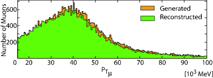
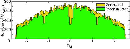
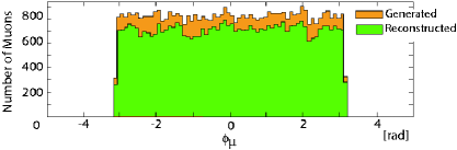
Figure 4: Distributions of the transverse momentum $P_{\mathrm{T\mu}}$, pseudorapidity $\eta_{\mu}$ and polar angle $\phi_{\mu}$ for muons from $\mathrm{b\bar{b}}$$\mathrm{Z}$($\ra$ $\mathrm{\mu^{+}\mu^{-}}$) Monte Carlo events, generated (brown) and both reconstructed (green) within the $|\eta|~{}\leq~{}2.5$ acceptance.

The distribution of the reconstructed dimuon invariant mass is shown in Fig. 5 (top) together with the result of a Gaussian fit. The solid line corresponds to the following values for the fit parameters:

$$<M^{\mathrm{inv}}_{\mu\mu}>=90.47\pm 0.05~{}\mathrm{Ge\kern-1.00006ptV}~{}~{}~{}~{}~{}\sigma(M^{\mathrm{inv}}_{\mu\mu})=3.02\pm 0.06~{}\mathrm{Ge\kern-1.00006ptV}\\$$ (3)

The fit mean is smaller than the nominal value of $m_{\mathrm{Z}}$ [29]. The $\mathrm{Z}$ natural width contributes to $\sigma(M^{\mathrm{inv}}_{\mu\mu})$ for approximately 1.9 $\mathrm{Ge\kern-1.00006ptV}$  thus implying a measurement accuracy $\sigma_{\rm res}=2.3~{}\mathrm{Ge\kern-1.00006ptV}$. This is just the value obtained unfolding the reconstructed distribution with the distribution of the $\mathrm{Z}$ generated mass, $M_{\rm gen}^{\mathrm{Z}}$. When the difference between reconstructed and generated mass $M^{\mathrm{inv}}_{\mu\mu}\ -M_{\rm gen}^{\mathrm{Z}}$ is plotted, Fig. 5 (bottom), the Gaussian fit of the distribution gives the following results for the fit parameters:

$$<M^{\mathrm{inv}}_{\mu\mu}-M_{\rm gen}^{\mathrm{Z}}>=-0.82~{}\pm~{}0.03~{}\mathrm{Ge\kern-1.00006ptV}~{}~{}~{}~{}\sigma_{\rm res}=2.35~{}\pm~{}0.03~{}\mathrm{Ge\kern-1.00006ptV}\\$$ (4)

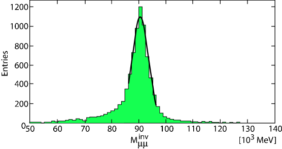
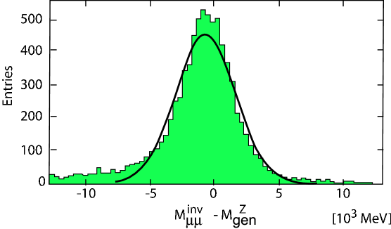
Figure 5: (top) Distribution of the invariant mass $M^{\mathrm{inv}}_{\mu\mu}$ reconstructed in $\mathrm{b\bar{b}}$$\mathrm{Z}$($\ra$ $\mathrm{\mu^{+}\mu^{-}}$) events. (bottom) Distribution of the difference between reconstructed and generated mass $M^{\mathrm{inv}}_{\mu\mu}-M^{\mathrm{Z}}_{\rm gen}$ for the same sample of events.

From this study we conclude that in the $m_{\mathrm{Z}}$  region the reconstructed $\mathrm{\mu^{+}\mu^{-}}$ invariant mass distribution shows a mean value shifted by 820 $\mathrm{Me\kern-1.00006ptV}$ with respect to the nominal value, towards the low mass region, and a resolution of $\sim$ 2.6 %. These results will be used later in Sec. 7.2.

6.2 b-tagging studies

The two b-tagging algorithms called 3D and SV2, which are in use within the ATLAS Collaboration [30], were studied with a subsample of $\mathrm{b\bar{b}}\mathrm{h}\rightarrow\mathrm{\mathrm{b\bar{b}}\mathrm{\mu^{+}\mu^{-}}}$ events.

Starting from the impact parameters (transverse and longitudinal) and their significances, both algorithms assign a weight to each track of the jet, that is to each track within a cone of opening angle $\Delta{\mathrm{R}}=\sqrt{\Delta\eta^{2}+\Delta\phi^{2}}$, with at least one track reconstructed in the tracker. The track weight is the ratio between the likelihood functions for a b-jet track and for a track of a light jet (from a light quark, u, d, s, c or a gluon). In turn the jet weight $\mathrm{w_{jet}}$ is defined as the sum of the logarithms of the tracks weights. This allows b-jets $(\rm w_{jet}>\rm w_{cut})$ to be discriminated against light jets ($\rm w_{jet}<\rm w_{cut}$) – the value $\rm w_{cut}$ is chosen, depending on the physics under study, such as to have a high efficiency $\epsilon_{\rm b}$ for b-jet identification and a high rejection factor $\rm{R_{j}}$ for light jets.

The SV2 algorithm improves on the 3D algorithm by using additional information on other variables not too strongly correlated with the impact parameters (as e.g. fraction of the jet energy and invariant mass of all particles at the secondary vertices, number of two-track secondary vertices).

In Table 4, the results of a study of a $\mathrm{b\bar{b}}\mathrm{h}\rightarrow\mathrm{\mathrm{b\bar{b}}\mathrm{\mu^{+}\mu^{-}}}$ sample are reported. Similar results have been obtained from a $\mathrm{b\bar{b}}\mathrm{Z}\rightarrow\mathrm{\mathrm{b\bar{b}}\mathrm{\mu^{+}\mu^{-}}}$ sample. For both samples, a selection cut, $P_{\mathrm{Tjet}}>15~{}\mathrm{Ge\kern-1.00006ptV}$, is applied, since below this value the efficiency of b-identification drops. The study is limited to the inner detector acceptance $|\eta|\leq 2.5$ and to two values of the jet opening angle, $\Delta{\mathrm{R}}=0.7$ and $\Delta{\mathrm{R}}=0.4$

Algorithm	$\Delta{\mathrm{R}}$	$\epsilon_{\rm b}$	$\rm{R_{j}}$	$\rm w_{cut}$	$\Delta{\mathrm{R}}$	$\epsilon_{\rm b}$	$\rm{R_{j}}$	$\rm w_{cut}$
SV2	0.7	49%	71	1	0.4	50%	58	1
3D	0.7	55%	27	1	0.4	54%	26	1
SV2	0.7	46%	219	2	0.4	46%	200	2
3D	0.7	49%	52	2	0.4	49%	50	2

Table 4: b-tag performance. The table shows, for the two algorithms used, the jet opening angle $\Delta{\mathrm{R}}$, the efficiency on b-jet identification $\epsilon_{\rm b}$, the rejection of light jets $\rm{R_{j}}$ and the value of $\rm w_{cut}$ (see text).

As results of this study, it is possible to conclude that:

• The SV2 algorithm, which uses more information on b decays products, provides a higher rejection rate with little loss in efficiency.

• No relevant improvement is obtained by shrinking the jet cone opening angle, $\Delta{\mathrm{R}}$, from 0.7 to 0.4. Therefore the ATHENA (v. 10.0.1) default value, $\Delta{\mathrm{R}}$=0.7, will be used in the following analysis.

• The cut value $\rm w_{cut}$ = 1 turns out to be a good compromise with a b-jet identification efficiency of $\approx$ 50% and a rejection of light jets by a factor of $\approx$ 70.

In case of high luminosity, possible track pileup doesn’t have a significant influence on b-tagging efficiency for this class of events. Their topology with two muons emerging from the primary vertex facilitates the selection of the correct primary vertex out of many interaction vertices.

6.3 Method for ${\boldsymbol{\mathrm{b\bar{b}}\mathrm{Z}\rightarrow\mathrm{\mathrm{b\bar{b}}\mathrm{\mu^{+}\mu^{-}}}}}$ background subtraction

The method proposed in [8] exploits the two following points (at the level of particle generation):
a) the rate of h/A $\ra\ee$ is expected to be suppressed with respect to the signal h/A $\ra\mathrm{\mu^{+}\mu^{-}}$ by a factor $\Big{(}\frac{m_{\mu}}{m_{e}}\Big{)}^{2}$,
b) the rate of the background $\mathrm{b\bar{b}}\mathrm{Z}\ra\mathrm{b\bar{b}}\mathrm{\mu^{+}\mu^{-}}$ is equal to the rate of $\mathrm{b\bar{b}}\mathrm{Z}\ra\mathrm{b\bar{b}}\ee$ because of the production diagrams which are the same, and of the lepton coupling universality in the Z decay.
In this context the associated $\mathrm{Z}$ production and decay in the channel $\mathrm{b\bar{b}}\mathrm{Z}\ra\mathrm{\mu^{+}\mu^{-}}$ has been studied using a control sample of $\mathrm{b\bar{b}}\mathrm{Z}\ra\ee$ events. The effect of inner bremsstrahlung (IB) radiation has been investigated and corrected for; the impact in the event reconstruction is not large. The ratio of the number of reconstructed events from the two samples in the region of mass higher than $m_{\mathrm{Z}}$, interesting for new physics search, is stable and implies correction factors close to one [8] .

As a result, barring corrections for different inner bremsstrahlung and detector response, the number of $\mathrm{b\bar{b}}\mathrm{Z}\ra\mathrm{b\bar{b}}\ee$ gives directly the number of background events $\mathrm{b\bar{b}}\mathrm{Z}\ra\mathrm{b\bar{b}}\mathrm{\mu^{+}\mu^{-}}$. Details of the method are given in Appendix A.

6.4 Significance of the search

Statistical methods used in Higgs boson searches are discussed in Ref. [31]. Here the significance of a search is given using $\frac{S}{\sqrt{B}}$ as a statistical estimator, where S is the number of signal events (h/A or h/A/H), and B the number of background events. Discovery means that the signal is larger than 5 times the background statistical error ($\frac{S}{\sqrt{B}}\geq 5$). The probability of a background fluctuation of this size is less than $\approx 2.87\cdot 10^{-7}$. A search resulting in $\frac{S}{\sqrt{B}}~{}\geq 3$ is interpreted as an indication of new physics.

7 Monte Carlo data analysis

7.1 ${\boldsymbol{\mathrm{b\bar{b}}\mathrm{A}\rightarrow\mathrm{\mathrm{b\bar{b}}\mathrm{\mu^{+}\mu^{-}}}},~{}\boldsymbol{\mathrm{b\bar{b}}\mathrm{h}\rightarrow\mathrm{\mathrm{b\bar{b}}\mathrm{\mu^{+}\mu^{-}}}},~{}\boldsymbol{\mathrm{b\bar{b}}\mathrm{H}\rightarrow\mathrm{\mathrm{b\bar{b}}\mathrm{\mu^{+}\mu^{-}}}}}$

The signature of the h/A channel is a pair of well isolated high-energy muons with opposite charge and two hadronic jets containing b quarks. The invariant mass of the reconstructed muons is supposed to originate from a h or A boson and must be compatible, within the mass resolution, with the corresponding mass, $m_{\mathrm{h}}$ or $m_{\mathrm{A}}$.

No simulation of the trigger is implemented; however two muons of transverse momentum above trigger experimental threshold are required and the detector acceptance considered is $|\eta|\leq 2.5$. The event selection is divided in three steps: preselection, tt veto selection, final selection.

The preselection, cuts 1-2-3 in Table 5, requires at least two well identified opposite charge muons with $P_{\mathrm{T\mu}}~{}\geq~{}10~{}\mathrm{Ge\kern-1.00006ptV}$ in the pseudo-rapidity range $|~{}\eta_{\mathrm{\mu}}|\leq~{}2.5$ (cut 1), thus satisfying the trigger requirement. The presence of a jet pair with $P_{\mathrm{Tjet}}\geq 10~{}\mathrm{Ge\kern-1.00006ptV}$ and $|~{}\eta_{\mathrm{jet}}|\leq~{}2.5$ is as well demanded, without any b-identification requirement (cut 2).

A further requirement (cut 3) is that at least one of these jets be identified as originating from a b-quark with $P_{\mathrm{Tjet}}>15$ $\mathrm{Ge\kern-1.00006ptV}$, that is the energy lower limit for a reliable b-jet identification [30] (Sec. 6.2). These cuts are designed to select events fulfilling the minimum conditions to be analyzed later. The events excluded are in any case not suitable to undergo any further analysis.

The tt veto selection  is designed to suppress this background, characterized by a large missing transverse energy due to the presence of neutrinos. $E^{\mathrm{miss}}_{\mathrm{T}}$ is required to be less than 45 GeV (cut 4). Other cuts (cut 5-6) are applied on the first and second most large muon transverse momentum, $P_{\mathrm{T\mu 1}}$ and $P_{\mathrm{T\mu 2}}$, and (cut 7-8) on the first and second most large jet transverse momentum, $P_{\mathrm{Tjet1}}$  and $P_{\mathrm{Tjet2}}$ . At least one of these jets was previously identified as originating from a b-quark (cut 3).

The final selection criteria are designed mainly to disentangle the signal events from the irreducible $\mathrm{Z}$ background. The main requirement is that the $\mathrm{\mu^{+}\mu^{-}}$ invariant mass has to lie inside a window around h/A mass, determined by the natural width of the bosons and by the experimental resolution of the $\mathrm{\mu^{+}\mu^{-}}$ invariant mass, Sec. 6.

The muons originating from b decays in bbbb events, with a cross section of $\approx 500$ pb [32], can mimic the signal events. To avoid this possible contamination a low hadronic activity near both muons is required. The isolation criteria demands that the sum of the charged track momenta in a cone ($\Delta{\mathrm{R}}<0.2$) around the muon direction be less than 5 $\mathrm{Ge\kern-1.00006ptV}$. These selection cuts are summarized in Table 5.

Cut Number	Variable
1	$N_{\mathrm{\mu}}~{}\geq~{}2,~{}P_{\mathrm{T\mu}}~{}\geq~{}10~{}\mathrm{Ge\kern-1.00006ptV},~{}|\eta_{\mathrm{\mu}}|~{}<2.5$
2	$N_{\mathrm{jet}}~{}\geq~{}2,~{}P_{\mathrm{Tjet}}~{}\geq~{}10~{}\mathrm{Ge\kern-1.00006ptV},~{}|\eta_{\mathrm{jet}}|~{}<2.5$
3	$N_{\mathrm{bjet}}~{}\geq~{}1,P_{\mathrm{Tjet}}~{}\geq~{}15~{}\mathrm{Ge\kern-1.00006ptV},~{}\mathrm{w_{btag}}~{}>1$
4	$E^{\mathrm{miss}}_{\mathrm{T}}~{}<45~{}\mathrm{Ge\kern-1.00006ptV}$
5	$25~{}\mathrm{Ge\kern-1.00006ptV}~{}<~{}P_{\mathrm{T\mu 1}}~{}<~{}95~{}\mathrm{Ge\kern-1.00006ptV}$
6	$20~{}\mathrm{Ge\kern-1.00006ptV}~{}<~{}P_{\mathrm{T\mu 2}}~{}<~{}60~{}\mathrm{Ge\kern-1.00006ptV}$
7	$P_{\mathrm{Tjet2}}~{}<40~{}\mathrm{Ge\kern-1.00006ptV}$
8	$P_{\mathrm{Tjet1}}~{}<70~{}\mathrm{Ge\kern-1.00006ptV}$
9	$|M^{\mathrm{inv}}_{\mu\mu}-m_{\mathrm{A}}|~{}\mathrm{or}~{}|M^{\mathrm{inv}}_{\mu\mu}-m_{\mathrm{h}}|<2\sigma$
10	$\Sigma|P_{\mathrm{Ttracks}}|~{}<~{}5~{}\mathrm{Ge\kern-1.00006ptV}~{}\mathrm{in~{}cone}~{}\Delta{\mathrm{R}}~{}<~{}0.2$

Table 5: Selection criteria for h/A $\ra\mathrm{\mu^{+}\mu^{-}}$ with two b-quarks final state.

A key point of the selection is the determination of the mass window used (cut 9). Its value is determined as a function of $\Gamma_{\mathrm{h}}$ ($\Gamma_{\mathrm{A}}$), the total width of the h (A) Higgs boson, and the experimental mass resolution $\sigma_{\rm m}$ = 2.6% (Sec. 6.1). The mass window is centered on the h (A) mass corrected for the bias k in the muon reconstruction, $m_{\mathrm{h},\rm{A}}^{\rm corr}=m_{\mathrm{h},\rm{A}}-\rm{k}$ with k= $-820$ $\mathrm{Me\kern-1.00006ptV}$ (Sec. 6.1). Its limits, $\xi_{\mathrm{h},\rm A}^{\pm}$, are defined by:

$$\xi_{\mathrm{h},\rm A}^{\pm}=m_{\mathrm{h},\rm{A}}^{\rm corr}\pm\rm{f}\cdot\Bigg{(}\bigg{(}\frac{\Gamma_{\mathrm{h},\rm{A}}}{2.36}\bigg{)}^{2}+\sigma^{2}_{\rm m}\Bigg{)}^{\frac{1}{2}},$$ (5)

where f is the standard deviation factor corresponding to a chosen probability. In our analysis f = 2, which corresponds to including 97.7% of the signal. The event is selected if the $\mathrm{\mu^{+}\mu^{-}}$ invariant mass is inside the window limits (5) either for the A or the h mass.

For the $\mathrm{b\bar{b}}\mathrm{H}\rightarrow\mathrm{\mathrm{b\bar{b}}\mathrm{\mu^{+}\mu^{-}}}$ channel the procedure is the same as for the h/A search, but for the selection window. The window limits are obtained from Eq. 5 with $m_{\mathrm{H}}$ (the H mass) replacing $m_{\mathrm{h},\rm{A}}$ in $m_{\mathrm{h},\rm{A}}^{\rm corr}$.

7.2 Reference point

The analysis procedure is first discussed for the reference point $m_{\mathrm{A}}$ = 110.31 $\mathrm{Ge\kern-1.00006ptV}$, $\mathrm{tan\beta}$ = 45 ($m_{\mathrm{h}}$ = 110.00 $\mathrm{Ge\kern-1.00006ptV}$, $m_{\mathrm{H}}$ = 127.46 $\mathrm{Ge\kern-1.00006ptV}$). For a given MSSM neutral Higgs boson (h, A, H) at this point, Table 6 shows the production cross section times the $\mathrm{\mu^{+}\mu^{-}}$ decay branching ratio, $\sigma_{\mathrm{b\bar{b}}\mathrm{\mu^{+}\mu^{-}}}$, the expected number of signal events at $\int\!{\cal L}\,\mathrm{d}t=300$ $\mathrm{fb^{-1}}$, $\rm N^{\rm exp_{300}}$, the number of Monte Carlo generated events $\rm N^{\rm MC}$ and their weight ${\rm w}$. The weight of the signal events is close to one as it is for all ($m_{\mathrm{A}}$, $\mathrm{tan\beta}$) points[7]. The background weights (Table 3) are also close to one.
We shall justify the cuts by showing examples of distributions obtained for the $\mathrm{b\bar{b}}\mathrm{h}\rightarrow\mathrm{\mathrm{b\bar{b}}\mathrm{\mu^{+}\mu^{-}}}$ signal and the $\mathrm{b\bar{b}}\mathrm{Z}\rightarrow\mathrm{\mathrm{b\bar{b}}\mathrm{\mu^{+}\mu^{-}}}$ background, and refer otherwise to [7] either for variables different from the ones displayed or for a different signal ($\mathrm{b\bar{b}}\mathrm{A}\rightarrow\mathrm{\mathrm{b\bar{b}}\mathrm{\mu^{+}\mu^{-}}}$ or $\mathrm{b\bar{b}}\mathrm{H}\rightarrow\mathrm{\mathrm{b\bar{b}}\mathrm{\mu^{+}\mu^{-}}}$) or for a different background ($\mathrm{t\bar{t}}\rightarrow\mathrm{\mathrm{b\bar{b}}\mathrm{\mu^{+}\mu^{-}}\mathrm{\nu\bar{\nu}}}$ or $\mathrm{Z}\mathrm{Z}\rightarrow\mathrm{\mathrm{b\bar{b}}\mathrm{\mu^{+}\mu^{-}}}$). In all cases the reconstructed distributions without cuts compare to the generated distributions as expected.

process	$\sigma_{\mathrm{b\bar{b}}\mathrm{\mu^{+}\mu^{-}}}$	$\rm N^{\rm exp_{300}}$	$\rm N^{\rm MC}$	${\rm w}$
(signal)	[pb]
$\mathrm{b\bar{b}}\mathrm{h}\rightarrow\mathrm{\mathrm{b\bar{b}}\mathrm{\mu^{+}\mu^{-}}}$	0.245	73500	76517	0.96
$\mathrm{b\bar{b}}\mathrm{A}\rightarrow\mathrm{\mathrm{b\bar{b}}\mathrm{\mu^{+}\mu^{-}}}$	0.2433	72900	74965	0.97
$\mathrm{b\bar{b}}\mathrm{H}\rightarrow\mathrm{\mathrm{b\bar{b}}\mathrm{\mu^{+}\mu^{-}}}$	0.001619	486	600	0.88

Table 6: h, A, H production at the reference point $\mathrm{tan\beta}$ = 45, $m_{\mathrm{A}}$ = 110.31 $\mathrm{Ge\kern-1.00006ptV}$($m_{\mathrm{h}}$ = 110.00 $\mathrm{Ge\kern-1.00006ptV}$, $m_{\mathrm{H}}$ = 127.46 $\mathrm{Ge\kern-1.00006ptV}$): process, cross section times $\mathrm{\mu^{+}\mu^{-}}$ decay branching ratio, $\sigma_{\mathrm{b\bar{b}}\mathrm{\mu^{+}\mu^{-}}}$, number of events expected for $\int\!{\cal L}\,\mathrm{d}t=300$ $\mathrm{fb^{-1}}$, ${\rm N^{\rm exp_{300}}}$, number of Monte Carlo generated events, ${\rm N^{\rm MC}}$, their weight w.

The distributions of the number of muons $N_{\mathrm{\mu}}$  and of the muon transverse momentum $P_{\mathrm{T\mu}}$ in the processes $\mathrm{b\bar{b}}\mathrm{h}\rightarrow\mathrm{\mathrm{b\bar{b}}\mathrm{\mu^{+}\mu^{-}}}$ and $\mathrm{b\bar{b}}\mathrm{Z}\rightarrow\mathrm{\mathrm{b\bar{b}}\mathrm{\mu^{+}\mu^{-}}}$ are displayed in Fig. 6 for the generated (hatched) and reconstructed (full color) events without any cut applied .

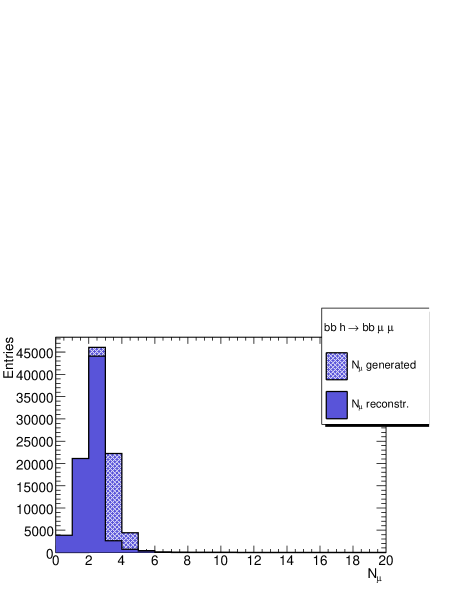
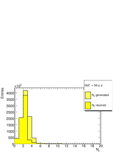
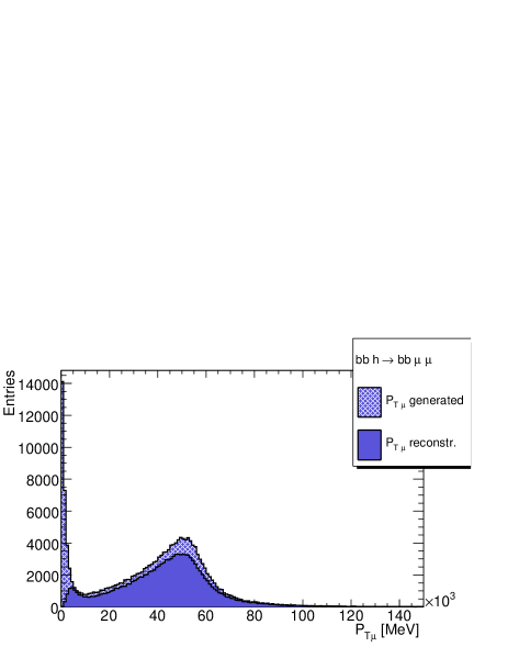
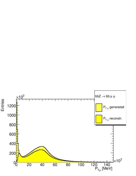
Figure 6: Without cut. Distributions of the number of muons $N_{\mathrm{\mu}}$ (top) and of the transverse momentum $P_{\mathrm{T\mu}}$ (bottom) for generated (hatched) and reconstructed (full color) events are plotted without cuts applied:
a) $\mathrm{b\bar{b}}\mathrm{h}\rightarrow\mathrm{\mathrm{b\bar{b}}\mathrm{\mu^{+}\mu^{-}}}$  events at the reference point ($\mathrm{tan\beta}$ = 45, $m_{\mathrm{h}}$ = 110.00 $\mathrm{Ge\kern-1.00006ptV}$)(left, dark blue); b) $\mathrm{b\bar{b}}\mathrm{Z}\rightarrow\mathrm{\mathrm{b\bar{b}}\mathrm{\mu^{+}\mu^{-}}}$ events (right, yellow). All distributions are normalized at $\int\!{\cal L}\,\mathrm{d}t$ = 300 $\mathrm{fb^{-1}}$. Entries are per bin width of 1 (top plots) and of $10^{3}$ MeV (bottom plots).

The preselection requirement on muon pair (cut 1, Table 5) reduces approximately to same fraction of signal ($\sim$ 62%) and background ($\mathrm{Z}$$\sim$ 59%, $\mathrm{t\bar{t}}$  $\sim$ 67%) events. The requirement on jet pair (cut 2) leaves almost untouched $\mathrm{t\bar{t}}$  ($\sim$ 63%) reducing $\mathrm{Z}$  to $\sim$ 54%, because of the more energetic $P_{\mathrm{Tjet}}$  spectra of the top decay [7]. Unfortunately for the same reason this cut reduces the signal sample significantly to $\sim$ 30% , see Table 7.

The mean jet transverse momentum $<P_{\mathrm{Tjet}}>$ is $\sim$ 26 $\mathrm{Ge\kern-1.00006ptV}$  for the h boson, and $\sim$ 36 $\mathrm{Ge\kern-1.00006ptV}$ for $\mathrm{Z}$  decays, see Fig. 7 [7]. Then, as stated in Sec. 3.3, the requirement that two b-jets be identified will not enhance the signal over this specific background. This requirement will suppress more the signal than the $\mathrm{Z}$ background, since the two b-jets of this background events are usually more energetic than those accompanying the signal. According to the study in Sec. 6.2, only one jet is required to be tagged as a b-jet.

After the three preselection cuts (1-2-3) the signal sample of h or A is reduced to $\sim$ 10%. The backgrounds are reduced to $\sim$ 17% for the $\mathrm{Z}$, $\sim$ 53% for $\mathrm{t\bar{t}}$, and $\sim$ 28% for $\mathrm{Z}$$\mathrm{Z}$.

The tt veto selection is designed to exploit features of t decays. The $\mathrm{t\bar{t}}$  sample is characterized by a transverse missing energy $E^{\mathrm{miss}}_{\mathrm{T}}$, which, due to neutrinos, is larger than in the h/A sample, as shown in Fig. 8. The $E^{\mathrm{miss}}_{\mathrm{T}}$ cut (cut 4, Table 5) is extremely effective, reducing $\mathrm{t\bar{t}}$  to $\sim$ 14 % of the original sample while keeping the signal at $\sim$ 9 % almost unchanged and the $\mathrm{Z}$ background at $\sim$ 14 %. The two cuts (5-6), related to $P_{\mathrm{T\mu}}$ distributions, reduce the $\mathrm{t\bar{t}}$ original sample to $\sim$ 8 %, but are little effective on the $\mathrm{Z}$ sample (to $\sim$ 10%) and the signal samples of h and A (to $\sim$ 8 %). A further reduction of the $\mathrm{t\bar{t}}$  background to 1.4 % is obtained by applying cuts (7-8) on $P_{\mathrm{Tjet}}$. At this stage, the $\mathrm{Z}$  sample is reduced to $\sim$ 5.8 % while the h signal as well as the A signal is reduced to 6.0 %, see Fig. 9.

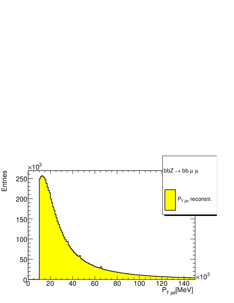
Figure 7: After 1-2 cuts. Distributions of the reconstructed jet transverse momentum $P_{\mathrm{Tjet}}$ are plotted after cuts 1 and 2 (Table 5) for :
a) $\mathrm{b\bar{b}}\mathrm{h}\rightarrow\mathrm{\mathrm{b\bar{b}}\mathrm{\mu^{+}\mu^{-}}}$ events at the reference point ($\mathrm{tan\beta}$  = 45, $m_{\mathrm{h}}$  = 110.00 $\mathrm{Ge\kern-1.00006ptV}$), (left, dark blue); b) $\mathrm{b\bar{b}}\mathrm{Z}\rightarrow\mathrm{\mathrm{b\bar{b}}\mathrm{\mu^{+}\mu^{-}}}$  events (right, yellow). All distributions are normalized at $\int\!{\cal L}\,\mathrm{d}t$ = 300 $\mathrm{fb^{-1}}$. Entries are per bin width of $10^{3}$ MeV.

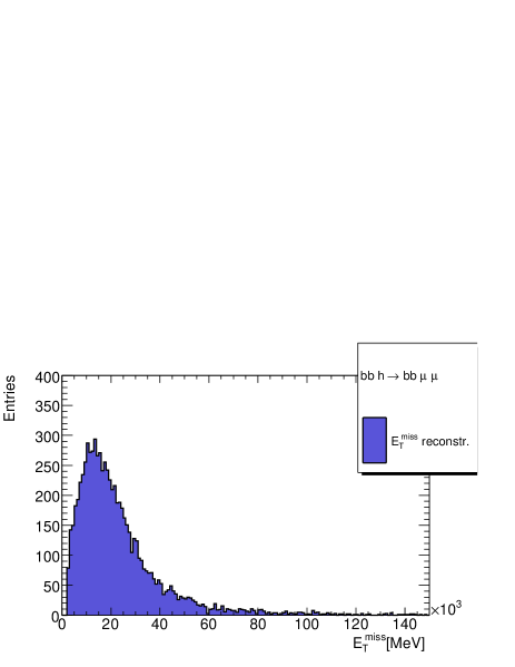
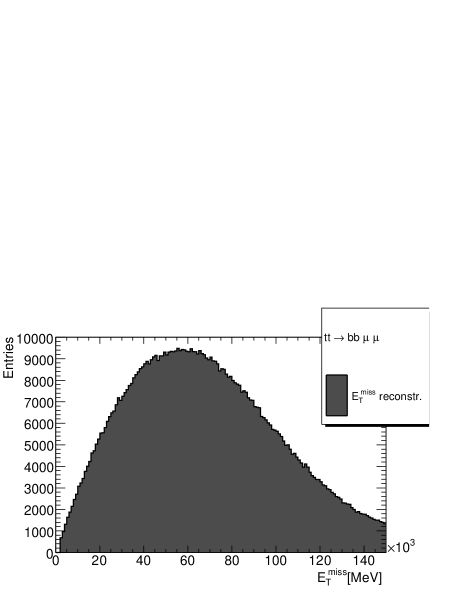
Figure 8: After 1-2-3 cuts. Distributions of the reconstructed transverse missing energy $E^{\mathrm{miss}}_{\mathrm{T}}$  are plotted after cuts 1, 2 and 3 (Table 5) for :
a) $\mathrm{b\bar{b}}\mathrm{h}\rightarrow\mathrm{\mathrm{b\bar{b}}\mathrm{\mu^{+}\mu^{-}}}$ events at the reference point ($\mathrm{tan\beta}$  = 45, $m_{\mathrm{h}}$  = 110.00 $\mathrm{Ge\kern-1.00006ptV}$), (left, dark blue); b) $\mathrm{t\bar{t}}\rightarrow\mathrm{\mathrm{b\bar{b}}\mathrm{\mu^{+}\mu^{-}}\mathrm{\nu\bar{\nu}}}$ events (right, gray). All distributions are normalized at $\int\!{\cal L}\,\mathrm{d}t$ = 300 $\mathrm{fb^{-1}}$. Entries are per bin width of $10^{3}$ MeV.

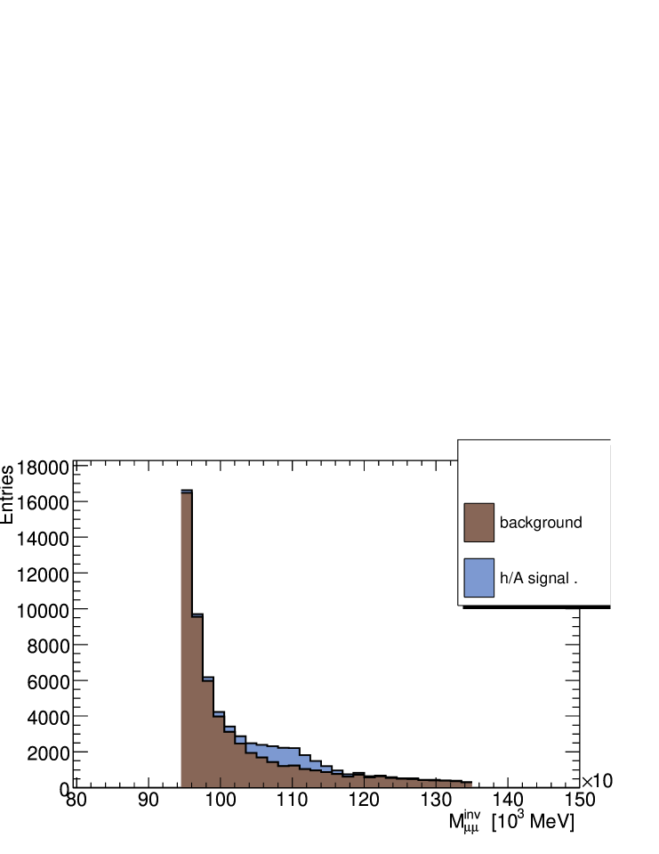
Figure 10: Distributions of the reconstructed $\mathrm{\mu^{+}\mu^{-}}$ invariant mass, $M^{\mathrm{inv}}_{\mu\mu}$, for signal and backgrounds events, after the selection cuts 1-8 (Table 5) at the reference point ($\mathrm{tan\beta}$ = 45, $m_{\mathrm{A}}$ = 110.31 $\mathrm{Ge\kern-1.00006ptV}$, $m_{\mathrm{h}}$ = 110.00 $\mathrm{Ge\kern-1.00006ptV}$). The two distributions are normalized at $\int\!{\cal L}\,\mathrm{d}t$= 300 $\mathrm{fb^{-1}}$. The h/A signal (light blue) emerge over the background ($\mathrm{Z}$, $\mathrm{t\bar{t}}$ and $\mathrm{Z}$$\mathrm{Z}$) (dark brown). Entries are per bin width of $1.5\cdot 10^{3}$ MeV.

The effect of cuts (1-8) is summarized in Fig. 10 which shows the distributions of the reconstructed $\mathrm{\mu^{+}\mu^{-}}$ invariant mass for signal (h and A) and (weighted) background (Z, $\mathrm{t\bar{t}}$ and ZZ added up) events. The h/A signal (light blue) is clearly visible on top of the remaining background events ($\mathrm{Z}$, $\mathrm{t\bar{t}}$ and $\mathrm{Z}$$\mathrm{Z}$ added up, dark brown).

To evaluate the significance of observation of a signal, the mass window (Eq. 5) is then selected, final selection (cut 9, Table 5). At the reference point ($m_{\mathrm{A}}$ = 110.31 $\mathrm{Ge\kern-1.00006ptV}$, $\Gamma_{\mathrm{A}}$ = 4.28 $\mathrm{Ge\kern-1.00006ptV}$ and $m_{\mathrm{h}}$ = 110.00 $\mathrm{Ge\kern-1.00006ptV}$, $\Gamma_{\mathrm{h}}$ = 4.20 $\mathrm{Ge\kern-1.00006ptV}$), Eq. 5 implies to look for the A signal in a window, $\xi_{\rm A}$, of 3.394 $\mathrm{Ge\kern-1.00006ptV}$ around a corrected mass value, $m_{\mathrm{A}}^{\rm corr}$, of 109.490 $\mathrm{Ge\kern-1.00006ptV}$, and for the h signal in a window, $\xi_{\mathrm{h}}$, of 3.369 $\mathrm{Ge\kern-1.00006ptV}$ around $m_{\mathrm{h}}^{\rm corr}$ = 109.180 $\mathrm{Ge\kern-1.00006ptV}$ (see [7] for the others values of $\mathrm{tan\beta}$, $m_{\mathrm{A}}$ and $m_{\mathrm{h}}$). As for the probability requirement f = 2, the windows $\xi_{\mathrm{h}}$ and $\xi_{\rm A}$ are increased by a factor 2 to obtain the effective selection window used in Table 9.

This selection reduces drastically the background samples, the $\mathrm{Z}$ to less than 0.13%, the $\mathrm{t\bar{t}}$ to 0.17 % and the $\mathrm{Z}$$\mathrm{Z}$ to a negligible 0.24 %. The event signal surviving in both A and h channels is $\approx$ 4.2 %.

The last reduction (cut 10) on muon isolation does not change significantly the previous results. Indeed this cut is expected to be effective in the data against the heavy flavour QCD background, and cannot be tested properly in Monte Carlo.

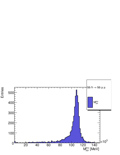
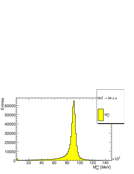
Figure 9: After 1-8 cuts. Distributions of the reconstructed $\mathrm{\mu^{+}\mu^{-}}$ invariant mass $M^{\mathrm{inv}}_{\mu\mu}$ are plotted after cuts 1 – 8 (Table 5) for:
a) $\mathrm{b\bar{b}}\mathrm{h}\rightarrow\mathrm{\mathrm{b\bar{b}}\mathrm{\mu^{+}\mu^{-}}}$ events at the reference point ($\mathrm{tan\beta}$  = 45, $m_{\mathrm{h}}$ = 110.00 $\mathrm{Ge\kern-1.00006ptV}$) (left, dark blue); b) $\mathrm{b\bar{b}}\mathrm{Z}\rightarrow\mathrm{\mathrm{b\bar{b}}\mathrm{\mu^{+}\mu^{-}}}$ events (right, yellow). All distributions are normalized at $\int\!{\cal L}\,\mathrm{d}t$ = 300 $\mathrm{fb^{-1}}$. Entries are per bin width of $1.5\cdot 10^{3}$ MeV.

Process	$\rm N^{\rm exp_{300}}$	$\rm N^{\rm MC}$	$\rm{N_{\rm 1cut}}$	$\rm{N_{\rm 2cut}}$	$\rm{N_{\rm 3cut}}$
$\mathrm{b\bar{b}}\mathrm{h}\rightarrow\mathrm{\mathrm{b\bar{b}}\mathrm{\mu^{+}\mu^{-}}}$	73500	76517	47099	22969	7907
$\mathrm{b\bar{b}}\mathrm{A}\rightarrow\mathrm{\mathrm{b\bar{b}}\mathrm{\mu^{+}\mu^{-}}}$	72900	74965	46247	22693	7919
$\mathrm{b\bar{b}}\mathrm{H}\rightarrow\mathrm{\mathrm{b\bar{b}}\mathrm{\mu^{+}\mu^{-}}}$	486	600	394	222	95
$\mathrm{b\bar{b}}\mathrm{Z}\rightarrow\mathrm{\mathrm{b\bar{b}}\mathrm{\mu^{+}\mu^{-}}}$	6836700	3314000	1945387	1178864	579751
$\mathrm{t\bar{t}}\rightarrow\mathrm{\mathrm{b\bar{b}}\mathrm{\mu^{+}\mu^{-}}\mathrm{\nu\bar{\nu}}}$	1713420	1806437	1217706	1137780	953928
$\mathrm{Z}\mathrm{Z}\rightarrow\mathrm{\mathrm{b\bar{b}}\mathrm{\mu^{+}\mu^{-}}}$	33819	97244	46487	38600	27744

Table 7: Preselection. Signal/Background process, number of events expected at $\int\!{\cal L}\,\mathrm{d}t=300~{}\mathrm{fb^{-1}}$, $\rm N^{\rm exp_{300}}$, number of Monte Carlo events generated, $\rm N^{\rm MC}$, and after three preselection steps, $\rm{N_{\rm 1cut}}$, $\rm{N_{\rm 2cut}}$ and $\rm{N_{\rm 3cut}}$ (Table 5). The signal is evaluated at the reference point ($\mathrm{tan\beta}$=45 , $m_{\mathrm{A}}$ = 110.31 $\mathrm{Ge\kern-1.00006ptV}$, $m_{\mathrm{h}}$ = 110.00 $\mathrm{Ge\kern-1.00006ptV}$). Cuts 1 to 3 are described in Table 5

Process	$\rm{N_{\rm 3cut}}$	$\rm{N_{\rm 4cut}}$	$\rm{N_{\rm 5cut}}$	$\rm{N_{\rm 6cut}}$	$\rm{N_{\rm 7cut}}$	$\rm{N_{\rm 8cut}}$
$\mathrm{b\bar{b}}\mathrm{h}\rightarrow\mathrm{\mathrm{b\bar{b}}\mathrm{\mu^{+}\mu^{-}}}$	7907	7099	6234	5575	5085	4636
$\mathrm{b\bar{b}}\mathrm{A}\rightarrow\mathrm{\mathrm{b\bar{b}}\mathrm{\mu^{+}\mu^{-}}}$	7919	7096	6183	5575	5118	4595
$\mathrm{b\bar{b}}\mathrm{H}\rightarrow\mathrm{\mathrm{b\bar{b}}\mathrm{\mu^{+}\mu^{-}}}$	95	78	66	54	50	44
$\mathrm{b\bar{b}}\mathrm{Z}\rightarrow\mathrm{\mathrm{b\bar{b}}\mathrm{\mu^{+}\mu^{-}}}$	579751	478106	397030	334609	226414	193334
$\mathrm{t\bar{t}}\rightarrow\mathrm{\mathrm{b\bar{b}}\mathrm{\mu^{+}\mu^{-}}\mathrm{\nu\bar{\nu}}}$	953928	256662	190672	143746	41954	25567
$\mathrm{Z}\mathrm{Z}\rightarrow\mathrm{\mathrm{b\bar{b}}\mathrm{\mu^{+}\mu^{-}}}$	27744	24516	19102	15957	10926	8574

Table 8: tt veto selection. Signal/Background process, number of Monte Carlo generated events after the preselection cut 3 and cuts 4 to 8. The signal is evaluated at the reference point ($\mathrm{tan\beta}$=45 , $m_{\mathrm{A}}$ = 110.31 $\mathrm{Ge\kern-1.00006ptV}$, $m_{\mathrm{h}}$ = 110.00 $\mathrm{Ge\kern-1.00006ptV}$). Cuts 3 to 8 are described in Table 5.

Process	$\rm{N_{\rm 8cut}}$	$\rm{N_{\rm 9cut}}$	$\rm{N_{\rm 10cut}}$
$\mathrm{b\bar{b}}\mathrm{h}\rightarrow\mathrm{\mathrm{b\bar{b}}\mathrm{\mu^{+}\mu^{-}}}$	4636	3212	3165
$\mathrm{b\bar{b}}\mathrm{A}\rightarrow\mathrm{\mathrm{b\bar{b}}\mathrm{\mu^{+}\mu^{-}}}$	4595	3151	3110
$\mathrm{b\bar{b}}\mathrm{H}\rightarrow\mathrm{\mathrm{b\bar{b}}\mathrm{\mu^{+}\mu^{-}}}$	44
$\mathrm{b\bar{b}}\mathrm{Z}\rightarrow\mathrm{\mathrm{b\bar{b}}\mathrm{\mu^{+}\mu^{-}}}$	193334	4496	4206
$\mathrm{t\bar{t}}\rightarrow\mathrm{\mathrm{b\bar{b}}\mathrm{\mu^{+}\mu^{-}}\mathrm{\nu\bar{\nu}}}$	25567	3148	2969
$\mathrm{Z}\mathrm{Z}\rightarrow\mathrm{\mathrm{b\bar{b}}\mathrm{\mu^{+}\mu^{-}}}$	8574	260	234

Table 9: Final selection. Signal/Background process, number of Monte Carlo generated events, after cut 8 and successive cuts 9 and 10. The signal is evaluated at the reference point ($\mathrm{tan\beta}$ = 45, $m_{\mathrm{A}}$ = 110.31 $\mathrm{Ge\kern-1.00006ptV}$, $m_{\mathrm{h}}$ = 110.00 $\mathrm{Ge\kern-1.00006ptV}$). Cuts 8 to 10 are described in Table 5 (see text for cut 9 window).

We calculate that the significance $\frac{S}{\sqrt{B}}$  at $\int\!{\cal L}\,\mathrm{d}t=300$ $\mathrm{fb^{-1}}$ is $\approx$ 56, scaling down to $\approx$ 18 at $\int\!{\cal L}\,\mathrm{d}t=30$ $\mathrm{fb^{-1}}$ and $\approx$ 10 at $\int\!{\cal L}\,\mathrm{d}t=10$ $\mathrm{fb^{-1}}$. As discussed in Sec. 3.3, the process of Z production accompanied by two light jets, which has not been simulated, can be an additional significant background. Its importance has been estimated from the relative cross-section and fake b-tagging probability. When this background is taken into account, we have estimated that the significance is lowered by $\approx$ 25%.

We conclude that if $m_{\mathrm{h}}$ = 110.00 $\mathrm{Ge\kern-1.00006ptV}$ and consequently $m_{\mathrm{A}}$ = 110.31 $\mathrm{Ge\kern-1.00006ptV}$ there is a high probability for these bosons to be discovered at the beginning of data taking.

8 Search in the MSSM plane

8.1 ${\boldsymbol{\mathrm{b\bar{b}}\mathrm{A}\rightarrow\mathrm{\mathrm{b\bar{b}}\mathrm{\mu^{+}\mu^{-}}}}}$, ${\boldsymbol{\mathrm{b\bar{b}}\mathrm{h}\rightarrow\mathrm{\mathrm{b\bar{b}}\mathrm{\mu^{+}\mu^{-}}}}}$

A search for neutral Higgs bosons h/A has been performed in the ($m_{\mathrm{A}}$, $\mathrm{tan\beta}$) plane, varying $\mathrm{tan\beta}$ between 15 and 50, in steps of 5, and $m_{\mathrm{h}}$ between 95 $\mathrm{Ge\kern-1.00006ptV}$ and 125 $\mathrm{Ge\kern-1.00006ptV}$, in steps of 2.5 GeV. For each point the statistics reached leads to weight factors for h and A boson close to unity.

The analysis described in Sec. 7 has been repeated for all 104 simulated points and the results are reported in Ref. [7].
The use of an asymmetric selection window, centered at $m_{\mathrm{h},\rm{A}}^{\rm corr}$ (see Sec. 7.1), has been tested for masses below 100 $\mathrm{Ge\kern-1.00006ptV}$, with a view to exclude the $\mathrm{Z}$ events, however without obtaining a significantly improved result ($\sim$ 10%). A symmetric window as described in Sec. 7.1 was thus applied to all masses.

The search significance for the h/A neutral boson is shown as a function of $m_{\mathrm{A}}$ up to highest allowed value of $m_{\mathrm{h}}$, in Fig. 11 for all scanned values of $\mathrm{tan\beta}$ and three luminosity, $\int\!{\cal L}\,\mathrm{d}t=300$ $\mathrm{fb^{-1}}$ ($S^{\mathrm{300}}_{\mathrm{h},~{}\mathrm{A}}$), 30 $\mathrm{fb^{-1}}$ ($S^{\mathrm{30}}_{\mathrm{h},~{}\mathrm{A}}$) and 10 $\mathrm{fb^{-1}}$ ($S^{\mathrm{10}}_{\mathrm{h},~{}\mathrm{A}}$)[7]. The values for the two lower luminosities were derived from the first one, which corresponds to the highest statistics..

One should note that large h/A masses are penalized by a small cross section, thus implying a lower significance, while the masses near to $m_{\mathrm{Z}}$  suffer from the difficulty in disentangling the neutral Higgs boson signal from the $\mathrm{Z}$ background.

The best mass range for an early discovery of h is between 100 and 120 $\mathrm{Ge\kern-1.00006ptV}$ at any given $\mathrm{tan\beta}$. If $\mathrm{tan\beta}>30$ a large range of masses is accessible to discovery even after the first year of data taking. More integrated luminosity, between $\approx$ 30 and 50 $\mathrm{fb^{-1}}$, is needed for $\mathrm{tan\beta}$  between 30 and 20. The discovery at $\mathrm{tan\beta}$ = 15 demands a luminosity of $\approx$ 150 $\mathrm{fb^{-1}}$, making the exploration of this region possible only after a few years of data taking.

These considerations are summarized in Fig. 12, where the minimum integrated luminosity $\int\!{\cal L}\,\mathrm{d}t$, demanded for a 5 $\sigma$ discovery of the h/A neutral Higgs boson, is plotted as a function of $m_{\mathrm{A}}$ up to highest allowed value of $m_{\mathrm{h}}$, at given $\mathrm{tan\beta}$ values. With a $\int\!{\cal L}\,\mathrm{d}t\approx 10$ $\mathrm{fb^{-1}}$, corresponding to one year of data taking, most of the masses are accessible if $\mathrm{tan\beta}>30$. More integrated luminosity is needed for $\mathrm{tan\beta}$  = 20 and $\mathrm{tan\beta}$  = 15. Low masses need as well more luminosity in order to extract the evidence of a signal from the most copious $\mathrm{Z}$ background.

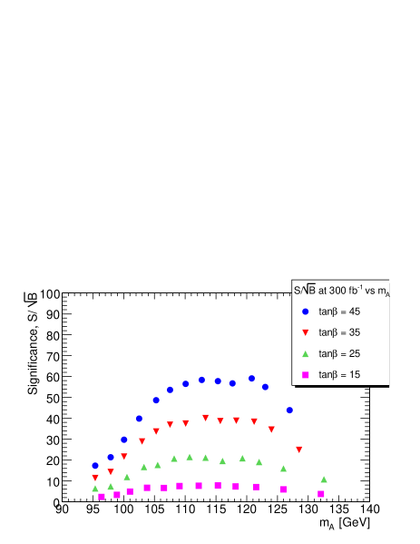
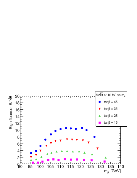
Figure 11: Search significance $\frac{S}{\sqrt{B}}$ for a h/A neutral Higgs boson, as a function of $m_{\mathrm{A}}$ up to the largest allowed value of $m_{\mathrm{h}}$  in three different data taking scenarios, $\int\!{\cal L}\,\mathrm{d}t$ = 300, 30 and 10 $\mathrm{fb^{-1}}$ (S is the number of h/A signal events, B is the number of background events). On the left the results for $\mathrm{tan\beta}$ = 50, 40, 30, 20, and on the right the results for $\mathrm{tan\beta}$ = 45, 35, 25, 15. The data are listed in Ref.[7].

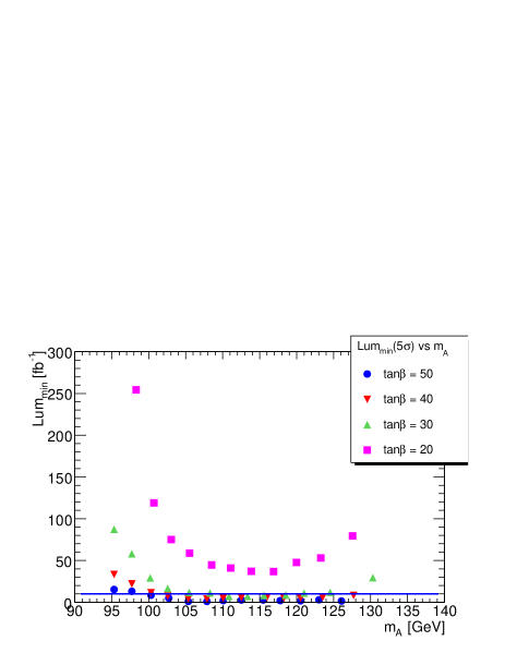
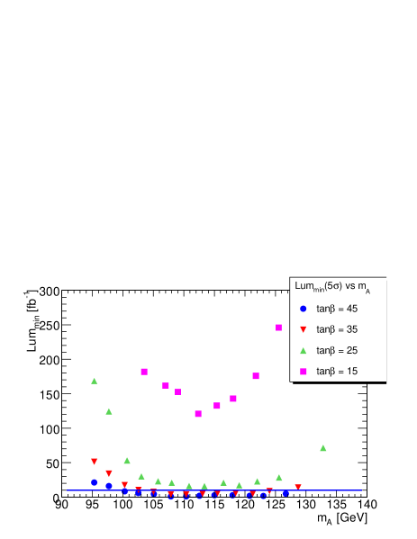
Figure 12: Minimum integrated luminosity $\int\!{\cal L}\,\mathrm{d}t$ demanded for a 5 $\sigma$ discovery of the h/A neutral Higgs boson as a function of $m_{\mathrm{A}}$ up to largest allowed value of $m_{\mathrm{h}}$. On the left the results for $\mathrm{tan\beta}$  = 50, 40, 30, 20, and on the right the results for $\mathrm{tan\beta}$  = 45, 35, 25, 15. The blue horizontal line is $\int\!{\cal L}\,\mathrm{d}t$ = 10 $\mathrm{fb^{-1}}$. The data are listed in Ref.[7] .

Discovery contours in the ($\mathrm{tan\beta}$, $m_{\mathrm{A}}$) plane are shown, in Fig. 13, in different $\int\!{\cal L}\,\mathrm{d}t$ scenarios for a significance of 5 (discovery, on the left) and of 3 (on the right). The latter can interpreted as the contour region for an early indication of a signal or, in case of negative search, for its exclusion.

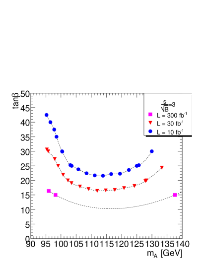
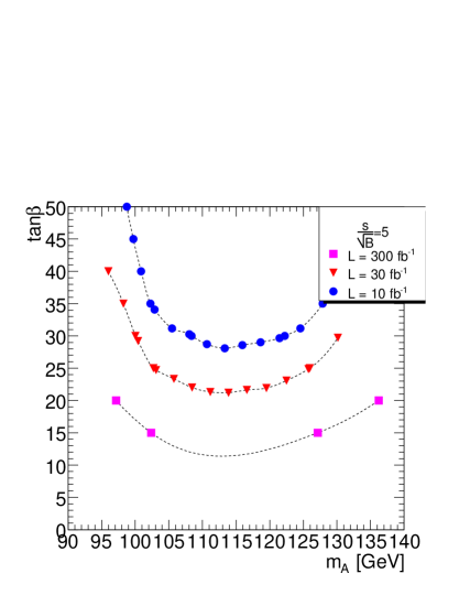
Figure 13: Discovery potential for a neutral Higgs boson h/A of mass $m_{\mathrm{A}}$ decaying to $\mathrm{\mu^{+}\mu^{-}}$, accompanied by two b-jets, in the $m_{\mathrm{h}}-{max}$ scenario (Sec. 2), as a function of $m_{\mathrm{A}}$: contours are drawn for a search significance $\frac{S}{\sqrt{B}}$  = 5 (left) and $\frac{S}{\sqrt{B}}$  = 3 (right), with an integrated luminosity of $\int\!{\cal L}\,\mathrm{d}t$ = 300 (top), 30 (center) and 10 (bottom) $\mathrm{fb^{-1}}$.

8.2 ${\boldsymbol{\mathrm{b\bar{b}}\mathrm{H}\rightarrow\mathrm{\mathrm{b\bar{b}}\mathrm{\mu^{+}\mu^{-}}}}}$

To increase the discovery potential for a neutral Higgs boson discovery in the region up 139 $\mathrm{Ge\kern-1.00006ptV}$ a search for the neutral Higgs boson H has been performed in the ($\mathrm{tan\beta}$, $m_{\mathrm{A}}$) plane inside the limits used for the h/A search (Sec. 8.1). This search required a separate analysis due to the higher mass region involved.

Due to the extremely low cross section of the H in this mass region, for a few masses with a cross section times $\mathrm{\mu^{+}\mu^{-}}$ branching ratio $\sigma_{\mathrm{H}}$$\cdot\rm{Br}_{\mathrm{\mu^{+}\mu^{-}}}$ smaller than 0.01 $\mathrm{pb}$, common values of center and selection window were chosen, corresponding to the mean values in that mass region. This procedure doesn’t affect any result due the narrow spread of values for the mass $m_{\mathrm{H}}$ and the natural width $\Gamma_{\mathrm{H}}$, implying that the window value is essentially dominated by the experimental resolution.

The discovery of the boson H demands a high integrated luminosity, $\int\!{\cal L}\,\mathrm{d}t\approx 300$ $\mathrm{fb^{-1}}$, and it would be possible at masses corresponding to $m_{\mathrm{h}}$ = 122.50 $\mathrm{Ge\kern-1.00006ptV}$ and 125 $\mathrm{Ge\kern-1.00006ptV}$ for values of $\mathrm{tan\beta}$ $\geq 30$. At $\mathrm{tan\beta}$ = 25, only a narrow range of $m_{\mathrm{H}}$ masses around 134 $\mathrm{Ge\kern-1.00006ptV}$ (corresponding to $m_{\mathrm{h}}$ = 125 $\mathrm{Ge\kern-1.00006ptV}$) is accessible. Lower values of $\mathrm{tan\beta}$ are excluded even at high masses.

In conclusion, a discovery of H boson is possible only in a few points of the parameter space, for a value of $m_{\mathrm{A}}$ around the maximum value of $m_{\mathrm{h}}$, at the ultimate luminosity expected at the LHC.

8.3 Combined search for ${\boldsymbol{\mathrm{b\bar{b}}\mathrm{A}\rightarrow\mathrm{\mathrm{b\bar{b}}\mathrm{\mu^{+}\mu^{-}}}}}$,
${\boldsymbol{\mathrm{b\bar{b}}\mathrm{h}\rightarrow\mathrm{\mathrm{b\bar{b}}\mathrm{\mu^{+}\mu^{-}}}}}$, ${\boldsymbol{\mathrm{b\bar{b}}\mathrm{H}\rightarrow\mathrm{\mathrm{b\bar{b}}\mathrm{\mu^{+}\mu^{-}}}}~{}}$

The results of Sec. 8.2 on the H boson search were combined with the results from the h/A search (Sec. 8.1). To this purpose, the H analysis was repeated with a window not overlapping with the h/A window, thus avoiding the double counting of background events. This work was performed only for high $m_{\mathrm{h}}$ values, where the cross section times the $\mathrm{\mu^{+}\mu^{-}}$ branching ratio (Sec. 8.2) has values $\geq$ 0.01 $\mathrm{pb}$ [7].

In Table 10 the significance of the exclusive search for the h/A boson ($S^{\mathrm{300}}_{\mathrm{h},~{}\mathrm{A}}$, $S^{\mathrm{30}}_{\mathrm{h},~{}\mathrm{A}}$, $S^{\mathrm{10}}_{\mathrm{h},~{}\mathrm{A}}$) and the corresponding significance including the H search ($S^{\mathrm{300}}_{\mathrm{h},~{}\mathrm{A},~{}\mathrm{H}}$, $S^{\mathrm{30}}_{\mathrm{h},~{}\mathrm{A},~{}\mathrm{H}}$  and $S^{\mathrm{10}}_{\mathrm{h},~{}\mathrm{A},~{}\mathrm{H}}$) at $\int\!{\cal L}\,\mathrm{d}t$ = 300, 30, 10 $\mathrm{fb^{-1}}$are shown.

The additional H search contributes to the MSSM Higgs sector discovery for $\mathrm{tan\beta}>15$ at the ultimate luminosity. Otherwise the contribution of this search is negligible, for a value of $m_{\mathrm{A}}$ around the maximum value of $m_{\mathrm{h}}$, as expected from the low cross section, and the large number of background events (being $m_{\mathrm{H}}$ close to $m_{\mathrm{Z}}$).

$\mathrm{tan\beta}$	$\bf{m_{\mathrm{h}}^{\rm nom}}$	$m_{\mathrm{H}}$	$S^{\mathrm{300}}_{\mathrm{h},~{}\mathrm{A}}$	$S^{\mathrm{30}}_{\mathrm{h},~{}\mathrm{A}}$	$S^{\mathrm{10}}_{\mathrm{h},~{}\mathrm{A}}$	$S^{\mathrm{300}}_{\mathrm{h},~{}\mathrm{A},~{}\mathrm{H}}$	$S^{\mathrm{30}}_{\mathrm{h},~{}\mathrm{A},~{}\mathrm{H}}$	$S^{\mathrm{10}}_{\mathrm{h},~{}\mathrm{A},~{}\mathrm{H}}$
	[$10^{\mathrm{3}}\mathrm{Me\kern-0.90005ptV}$]	[$\mathrm{Me\kern-0.90005ptV}$]
15	122.50	136180	3.86	1.22	0.70	5.09	1.64	0.93
15	125.00	152610	1.51	0.48	0.28	2.27	0.73	0.19
20	122.50	131870	9.76	3.08	1.78	11.69	3.77	2.14
20	125.00	139490	4.63	1.47	0.85	7.25	2.34	0.76
25	122.50	130020	15.98	5.05	2.92	17.51	5.65	3.2
25	125.00	134420	10.27	3.25	1.88	15.20	4.9	2.78
30	122.50	129090	25.13	7.95	4.59	27.01	8.71	4.94
30	125.00	131890	16.13	5.10	2.95	22.88	7.36	4.18
35	122.50	128560	34.71	10.97	6.34	35.29	11.38	6.45
35	125.00	130470	24.18	7.65	4.41	32.66	10.54	5.09
40	122.50	128260	43.68	13.81	7.98	43.95	14.18	8.03
40	125.00	129610	34.02	10.76	6.21	43.56	14.05	7.96
45	120.00	127790	59.03	18.67	10.78	54.16	17.47	9.90
45	122.50	128090	54.70	17.30	9.99	54.61	17.62	9.98
45	125.00	129090	43.54	13.77	7.95	53.90	17.38	9.85
50	120.00	127780	67.10	21.22	12.25	60.72	19.59	11.10
50	122.50	128020	65.55	20.73	11.97	65.27	21.10	11.93
50	125.00	128760	56.16	17.76	10.25	66.70	21.52	12.19

Table 10: Significance of A/h and A/h/H searches. The significance values for the two searches, $S^{\mathrm{300}}_{\mathrm{h},~{}\mathrm{A}}$, $S^{\mathrm{30}}_{\mathrm{h},~{}\mathrm{A}}$, $S^{\mathrm{10}}_{\mathrm{h},~{}\mathrm{A}}$and $S^{\mathrm{300}}_{\mathrm{h},~{}\mathrm{A},~{}\mathrm{H}}$, $S^{\mathrm{30}}_{\mathrm{h},~{}\mathrm{A},~{}\mathrm{H}}$, $S^{\mathrm{10}}_{\mathrm{h},~{}\mathrm{A},~{}\mathrm{H}}$, at $\int\!{\cal L}\,\mathrm{d}t$ = 300, 30, 10 $\mathrm{fb^{-1}}$, respectively, are given for a set of $\mathrm{tan\beta}$ values and two values of the mass of the lightest neutral Higgs boson, $m_{\mathrm{h}}^{\rm nom}$. The mass $m_{\mathrm{H}}$ of the corresponding H Higgs boson is also noted.

9 Conclusions

The possibility of the discovery of the MSSM h/A bosons in the region of high $\mathrm{tan\beta}$ ( larger than 15) and mass close to 100 $\mathrm{Ge\kern-1.00006ptV}$ has been investigated by exploiting the decay of the neutral h/A boson into two muons, $\mathrm{h}$$\ra\mathrm{\mu^{+}\mu^{-}}$ and $\mathrm{A}$$\ra\mathrm{\mu^{+}\mu^{-}}$ , accompanied by two b-jets. This region is also accessible by charged MSSM Higgs boson $\mathrm{H^{\pm}}$ decays.

For this purpose an analysis using full detector simulation has been performed. Monte Carlo events have been generated for a center-of-mass energy $\sqrt{s}$= 14 $\mathrm{Te\kern-1.00006ptV}$ through the ATHENA interface (v.9.0.4), while the ATLAS detector response has been simulated using the GEANT program through the ATHENA interface (v.10.0.1).

The results described in this paper show a well defined possibility for the discovery of a neutral Higgs boson in a region traditionally difficult due to the presence of the $\mathrm{Z}$ resonance.

This is achieved thanks to the high resolution performance of the ATLAS detector, namely of the muon spectrometer and the inner detector, together with the high b-tagging capability. For completeness the search of H$\ra\mathrm{\mu^{+}\mu^{-}}$ has been explored in the same mass region.

The discovery of a neutral MSSM boson looks possible in a mass range of 100 to 120 GeV at $\mathrm{tan\beta}>15$, with an integrated luminosity $\int\!{\cal L}\,\mathrm{d}t$ = 10 $\mathrm{fb^{-1}}$, which corresponds to one year of data taking. A warning should be made however because of unaccounted uncertainties in background and other systematic errors that cannot be evaluated precisely at this time.

With a view to perform this analysis on real data a method to subtract the main contributing background of Z boson decays Z $\mathrm{\mu^{+}\mu^{-}}$ has been suggested by us [8]. This method mainly relies on experimental data with limited Monte Carlo corrections. The procedure is based on the use of a control sample of Z bosons decaying to electrons, and does not depend on complex theoretical calculations nor on their implementation in Monte Carlo.

10 Acknowledgments

This work has been performed withins ATLAS Collaboration and we thank collaboration members for helpful discussions. We have made use of physics analysis framework and tools which are the result of collaboration-wide efforts.

Appendix A Appendix:
subtraction of the ${\boldsymbol{\mathrm{b\bar{b}}\mathrm{Z}\rightarrow\mathrm{\mathrm{b\bar{b}}\mathrm{\mu^{+}\mu^{-}}}}}$ background

Following the method outlined in Sec. 6.3 and based on the universality of the lepton coupling, the number of background events $\mathrm{b\bar{b}}\mathrm{Z}\rightarrow\mathrm{\mathrm{b\bar{b}}\mathrm{\mu^{+}\mu^{-}}}$, $N_{\mathrm{Z}\ra\mathrm{\mu^{+}\mu^{-}}}$, is given by the number, $N_{\mathrm{Z}\ra\ee}$, of $\mathrm{b\bar{b}}$$\mathrm{Z}$ events collected in the same real data sample. In both cases the number of events is the one counted within a window of the two-lepton invariant mass distribution. The method has been fully proved with the simulation described in [8].

The ratio $N_{\mathrm{Z}\ra\mathrm{\mu^{+}\mu^{-}}}/N_{\mathrm{Z}\ra\ee}$ has been shown to be a regular function of the dilepton invariant mass in the region of interest between 97.5 $\mathrm{Ge\kern-1.00006ptV}$ and 140 $\mathrm{Ge\kern-1.00006ptV}$ once possible sources of differences between  and $\mathrm{\mu^{+}\mu^{-}}$ data have been taken into account, and to be close to one. We like to recall here these differences and their impact on the above ratio.

Clearly, depending on whether the final state contains electrons or muons, one has to provide for the differences in the detector response that is for the acceptance and resolution of the electromagnetic calorimeter and the muon spectrometer.

Since our samples are $\mathrm{b\bar{b}}\mathrm{Z}\ra\mathrm{\mu^{+}\mu^{-}}$ or $\mathrm{b\bar{b}}\mathrm{Z}\ra\ee$, in those events where a semileptonic b decay occurs with the same flavour as one of the $\mathrm{Z}$ decay products, more than one invariant mass combination is possible, namely three (only opposite charge lepton pairs are considered for invariant mass combinations). Often, the value of the invariant mass associated to this combination of one lepton originating from $\mathrm{Z}$ and another one from b decay sits far from $m_{\mathrm{Z}}$ (and thus has no effect in the interested region). However the higher efficiency in muon detection increases the number of fake combinations in the muon sample.

Less obvious are the corrections required by the different inner bremsstrahlung in the two samples. The inner bremsstrahlung (IB) is the emission of photons, $\gamma_{\mathrm{brem}}$, near the Z or Z$\mathrm{\mu^{+}\mu^{-}}$ vertex. The presence of such photons changes the kinematic configuration of the decay, in particular the lepton 4-momenta. The impact of this effect on the Higgs mass resolution with the ATLAS detector has been studied in Ref.[33]. Here we discuss its impact on the number of detected events as a function of the dilepton reconstructed invariant mass in the region of our search.

At the generator level in the electron (muon) sample 85.2% (91.6%) of the events are without IB photons, 13.7% (8%) have 1 $\gamma_{\mathrm{brem}}$, 0.94% (0.2%) have 2 $\gamma_{\mathrm{brem}}$. The corresponding average transverse momentum of the radiated photons, without any cut except those mentioned in Sec. 4, is close in the two samples, $<P_{\mathrm{T}}^{\gamma_{\mathrm{brem}}}>=16.18~{}\mathrm{Ge\kern-1.00006ptV}$ for the  sample and $<P_{\mathrm{T}}^{\gamma_{\mathrm{brem}}}>=16.43~{}\mathrm{Ge\kern-1.00006ptV}$ for the $\mathrm{\mu^{+}\mu^{-}}$ sample. These IB photons are mainly contained in a cone with an opening $\Delta{\mathrm{R}}=0.15$ around a muon track and $\Delta{\mathrm{R}}=0.25$ around an electron track. By summing up the IB photon 4-momentum to the close lepton 4-momentum one obtains that the ratio $N_{\mathrm{Z}\ra\mathrm{\mu^{+}\mu^{-}}}/N_{\mathrm{Z}\ra\ee}$ stays the same within $\pm 12\%$ for dilepton invariant masses between 100 and 140 $\mathrm{Ge\kern-1.00006ptV}$. It would otherwise show a spread of $\approx\pm 30\%$.

At the detector level muons, electrons and photons involve different detectors (muon spectrometer and electromagnetic calorimeter) implying different momentum resolution, angular acceptance and efficiency. In this analysis we used identification criteria as follows.

A muon is reconstructed as a track, in both the inner detector and the muon spectrometer (so named combined reconstruction), and enters the analysis if $P_{\mathrm{T}}>10~{}\mathrm{Ge\kern-1.00006ptV}$ and $|\eta|<2.5$. The average momentum reconstructed is $<P_{\mathrm{T}}>=37.83~{}\mathrm{Ge\kern-1.00006ptV}$. The reconstruction efficiency is higher for muons than for electrons.

An electron is reconstructed as a cluster in the electromagnetic calorimeter associated with a track inside $\Delta\eta=0.025$ and $\Delta\phi=0.05$, and enters the analysis if $P_{\mathrm{T}}>10~{}\mathrm{Ge\kern-1.00006ptV}$ and $|\eta|<2.5$. The best performance is achieved when the energy is measured in the electromagnetic calorimeter (with a cluster size of $5\times 5$ cells) and the angles ($\theta,\phi$) in the tracker. The average momentum reconstructed is $<P_{\mathrm{T}}>=42.61~{}\mathrm{Ge\kern-1.00006ptV}$.

A photon is reconstructed as a cluster in the electromagnetic calorimeter not associated to any track inside $\Delta\eta=0.025$ and $\Delta\phi=0.05$, and enters the analysis if $E_{{\rm T}}>10~{}\mathrm{Ge\kern-1.00006ptV}$ and $|\eta|<2.5$. A cluster size of 5$\times$5 cells is used to measure the energy. The value chosen for the $E_{{\rm T}}$ threshold ensures a good photon reconstruction efficiency.

In this analysis however a photon’s 4-momentum is summed with that of the lepton if the photon is reconstructed inside a cone $\Delta{\mathrm{R}}<0.15$ around an electron ( sample) or $\Delta{\mathrm{R}}<0.25$ around a muon ($\mathrm{\mu^{+}\mu^{-}}$ sample). As a result, although the number of photons of any origin is more important in the  than in the $\mathrm{\mu^{+}\mu^{-}}$ sample, the number of photons reconstructed separately is equal ($\sim 1\%$) in the two samples. The effect of summing the photon and lepton 4-momenta shows up in the distribution of the ratio $N_{\mathrm{\mu^{+}\mu^{-}}}/N_{\ee}$ as a function of the dilepton invariant mass when only events containing an IB photon at the generator level are considered. It consists in a shift from the low-mass tail towards the $\mathrm{Z}$ mass.

Based on the whole simulation we could conclude [8] that the ratio $N_{\mathrm{\mu^{+}\mu^{-}}}/N_{\ee}$ is $\approx 1.2$ and does not depend, in the region of our search and within the simulation statistics, on the two-lepton invariant mass.

References

- [1] H.-P. Nilles, Phys. Rep. 110 (1984) 1.
- [2] H. E. Haber and G. L. Kane, Phys. Rep. 117 (1985) 75.
- [3] R. Barbieri, Riv. Nuovo Cim. 11 (1988) n. 4.
- [4] ALEPH Collaboration, DELPHI Collaboration, L3 Collaboration, OPAL Collaboration and LEP Working Group for Higgs boson searches, Phys. Lett. B565 (2003) 61.
- [5] The LEP Collaborations ALEPH, DELPHI, L3 and OPAL, and LEP Working Group for Higgs boson searches, Eur. Phys. J. C47 (2006) 547.
- [6] ALEPH, DELPHI, L3, OPAL Collaboration and LEP Working Group for Higgs boson searches, Search for charged Higgs bosons: Preliminary combined results using LEP data collected at energies up to 209 GeV, 2001, hep-ex/0107031.
- [7] S. Gentile, H. Bilokon, V. Chiarella, G. Nicoletti, Search for MSSM neutral Higgs bosons decaying to a muon pair in the mass range up to 130 GeV, 2007, Università La Sapienza, Sez. I.N.F.N., Roma, Laboratori Nazionali di Frascati, I.N.F.N, Frascati Italy, ATL-PHYS-PUB-2007-001.
- [8] S. Gentile, H. Bilokon, V. Chiarella, G. Nicoletti, Data based method for background subtraction in ATLAS detector at LHC, 2006, Università La Sapienza, Sez. I.N.F.N., Roma, Laboratori Nazionali di Frascati, I.N.F.N, Frascati Italy, ATL-PHYS-PUB-2006-019.
- [9] Stephen P. Martin, A supersymmetry primer, 1997, hep-ph/9709356.
- [10] E. Richter-Was \etal, Int. J. Mod. Phys. A13 (1998) 1371.
- [11] V. Abazov, Phys. Rev. Lett. 95 (2005) 151801.
- [12] A. Abulenci, Phys. Rev. Lett. 96 (2006) 011802.
-
[13]
ATLAS Coll., ATLAS detector and Physics Performance:
Technical Design Report, Volume 2,
report CERN/LHCC/99-15 (1999). -
[14]
CMS Coll., CMS detector and Physics Performance:
Physics Technical Design Report, Volume 1,
report CERN/LHCC/2006-001 (2006). - [15] K.A. Assamagan, \etal, Eur. Phys. J. direct C4 (2002) 9.
- [16] M. Schumacher, Investigation of the discovery potential for Higgs bosons of the minimal supersymmetric extension of the standard model (MSSM) with ATLAS, 2004, hep-ph/0410112.
- [17] B. P. Kersevan and E. Richter-Was, The Monte Carlo event generator AcerMC version 2.0 with interfaces to PYTHIA 6.2 and HERWIG 6.5, 2004, hep-ph/0405247.
- [18] T. Sjostrand, L. Lonnblad and S. Mrenna, PYTHIA 6.226: Physics and manual, 2004, hep-ph/0405247.
- [19] T.Gleisberg \etal, JHEP 02 (2004) 056.
- [20] S. Agostinelli \etal, Nucl. Instrum. Methods Phys. Res. A 506 (2003) 250.
- [21] J. Alison \etal, IEEE Transactions on Nuclear Science 53 (2006) 270.
- [22] S. Mrenna, 2005, Private Communication.
- [23] J. Campbell and R.K. Ellis and D.L. Rainwater, Phys. Rev. D68 (2003) 094021.
-
[24]
ATLAS Coll., ATLAS detector and Physics Performance:
Technical Design Report, Volume 1,
report CERN/LHCC/99-15 (1999). - [25] D. Froidevaux and P. Sphicas, Ann. Rev. Nucl. Part. Sci. 56 (2006) 375–440.
- [26] E. Pomarico, Studio del Processo di decadimento del bosone nel canale , 2005, Università La Sapienza, Roma.
- [27] D. Adams, 2006, Private Communication.
- [28] S. Rosati, H 4 leptons, 2005, Atlas Physics workshop, 6-11 June 2005, Rome.
- [29] W.-M. Yao \etal, J. Phys. G33 (2006) 1.
- [30] S. Corréard, V. Kostioukhine, J. Levêque, A. Rozanov, J.-B. de Vivie, b-tagging with DC1 data, 2003, ATL-COM-PHYS-2003-049.
- [31] K. S. Cranmer, B. Mellado, W. Quayle and Sau Lan Wu, ECONF C030908 (2003) MODT004.
- [32] M. L. Mangano, M. Moretti, F. Piccinini, R. Pittau and A. D. Polosa, JHEP 07 (2003) 001.
- [33] O. Linossier, L. Poggioli, Final State inner-bremsstrahlung effetcs on channel with ATLAS, 1995, LAPP, Annecy-le-Vieux, France, CERN, Geneva, Switzerland, ATLAS Internal note, Phys No 075.