2006

Chapter 1 Introducion

1.1 That is a base of astrophysics?

The empirical testing of a scientific hypothesis is the main instrument of the present exact science. It was founded by G.Galileo and his contemporaries. False scientific statements weren’t afraid of an empirical testing up to that time. A flight of fancy was far refined than an ordinary and crude material world. The exact correspondence of philosophical theory to a check experiment was not necessary, it almost discredits the theory in an esoteric opinion. The discrepancy of a theory and observations was not confusing at that time. Now the empirical testing of all theoretical hypotheses gets a generally accepted obligatory method of exact science. As a result all basic statements of physics are sure established. The situation in astrophysics is quite different .

Sometimes one considers the astrophysics as a division of science where quantities 1, 10 and 100 are equivalent, and a comparison of astrophysical models to measured astronomical data is impossible according to this reason and is not required. From its initial stage the astrophysics was developed under assumption that its statements are practically impossible to check. A long time this science uses surely established ”terrestrial” physical laws to obtain its results, and it was a restriction of its empirical testing. On the base of these experimentally tested ”terresrial” laws, astrophysicists obtain their conclusions about properties and internal structures of distant and mysterious stars without any hope to check these theoretical constructions. This point of view was clearly expressed by O.Kont (France,1798-1857):

”We don’t know anything about stars, except they are exist. Even their temperatures stay indefinite forever”

(O.Kont ”The philosophical treatise about a popular astronomy”, 1844.)

Later temperatures of stars and many other of their parameters were measured, but it did not make progress in checking of astrophysical models. It is supposed that it is enough to use surely established physical laws to obtain correct description of a star interior. The astrophysical community is in the firm belief that the basis of this science is surely formulated. .

But the correctness of a fundamental scientific problem can not be based on a belief or on an intuition and must not be solved by voting of professionals. Fortunately, the situation was greatly changed in the last decades of 20th century. In according to the progress a measuring technics, astronomers obtain the important data. They give a possibility to check a basis of astrophysical models. This testing will be made below.

1.2 The basic postulate of astrophysics

The basic postulate of astrophysics - the Euler equation - was formulated in a mathematical form by L.Euler in a middle of 18th century for the ”terrestrial” effects description. This equation determines the equilibrium condition of liquids or gases in a gravitational field:

$$\gamma{\mathbf{g}}=-{\mathbf{\nabla}}P.$$ (1.1)

According to it the action of a gravity forth $\gamma{\mathbf{g}}$ ($\gamma$ is density of substance, ${\mathbf{g}}$ is the gravity acceleration) in equilibrium is balanced by a forth which is induced by the pressure gradient in the substance. This postulate is surely established and experimentally checked be ”terrestrial” physics. It is the base of an operating of series of technical devices - balloons, bathyscaphes and other.

All modern models of stellar interior are obtained on the base of the Euler equation. These models assume that pressure inside a star monotone increases depthward from the star surface. As a star interior substance can be considered as an ideal gas which pressure is proportional to its temperature and density, all astrophysical models predict more or less monotonous increasing of temperature and density of the star substance in the direction of the center of a star.

1.3 The Galileo’s method

The correctness of fundamental scientific postulate has to be confirmed by empirical testing. The basic postulate of astrophysics - the Euler equation (Eq.(1.1)) - was formulated long before the plasma theory has appeared, even long before the discovering of electrons and nuclei. Now we are sure that the star interior must consist of electron-nuclear plasma. The Euler equation describes behavior of liquids or gases - substances, consisting of neutral particles. One can ask oneself: must the electric interaction between plasmas particles be taken into account at a reformulation of the Euler equation, or does it give a small correction only, which can be neglected in most cases, and how is it accepted by modern stellar theories?

To solve the problem of the correct choice of the postulate, one has the Galileo’s method. It consists of 3 steps:

(1) to postulate a hypothesis about the nature of the phenomenon, which is free from logical contradictions;

(2) on the base of this postulate, using the standard mathematical procedures, to conclude laws of the phenomenon;

(3) by means of empirical method to ensure, that the nature obeys these laws (or not) in reality, and to confirm (or not) the basic hypothesis.

The use of this method gives a possibility to reject false postulates and theories, provided there exist a necessary observation data, of course.

The modern theory of the star interior is based on the Euler equation Eq.(1.1). Another possible approach is to take into account all interactions acting in the considered system. Following this approach one takes into account in the equilibrium equation the electric interactions too, because plasma particles have electric charges. An energetic reason speaks that plasma in gravity field must stay electroneutral and surplus free charges must be absent inside it.The gravity action on a neutral plasma may induce a displacements of its particles, i.e. its electric polarization, because electric dipole moments are lowest moments of the analysis of multipoles. If we take into account the electric polarization plasma $\mathfrak{P}$, the equilibrium equation obtains the form:

$$\gamma\mathbf{g}+\frac{4\pi}{3}\mathfrak{P}\nabla\mathfrak{P}+\mathbf{\nabla}P=0,$$ (1.2)

On the basis of this postulate and using standard procedures, the star interior structure can be considered (it is the main substance of this paper).

Below it will be shown that the electric force in a very hot dense plasma can fully compensate the gravity force and the equilibrium equation then obtains the form:

$$\gamma\mathbf{g}+\frac{4\pi}{3}\mathfrak{P}\nabla\mathfrak{P}=0$$ (1.3)

and

$$\mathbf{\nabla}P=0,$$ (1.4)

which points to a radical distinction of this approach in comparison to the standard scheme based on Eq.(1.1).

1.4 What does the the astronomic measurement data express?

Are there actually astronomic measurement data, which can give possibility to distinguish ”correct” and ”incorrect” postulates? What must one do, if the direct measurement of the star interior construction is impossible?

Are there astronomical measurement data which can clarity this problem? Yes. They are:

1. There is the only method which gives information about the distribution of the matter inside stars. It is the measurement of the periastron rotation of closed double stars. The results of these measurements give a qualitative confirmation that the matter of a star is more dense near to its center.

2. There is the measured distribution of star masses. Usually it does not have any interpretation.

3. The astronomers detect the dependencies of radii of stars and their surface temperatures from their masses. Clear quantitative explanations of these dependencies are unknown.

4. The existence of these dependencies leads to a mass-luminosity dependence. It is indicative that the astrophysical community does not find any quantitative explanation to this dependence almost 100 years after as it was discovered.

5. The discovering of the solar surface oscillations poses a new problem that needs a quantitative explanation.

6. There are measured data showing that a some stars are possessing by the magnetic fields. This date can be analyzed at taking into account of the electric polarization inside these stars.

It seems that all measuring data are listed which can determine the correct choice of the starting postulate.

It is important to underline that all above-enumerated dependencies are known but they don’t have a quantitative (often even qualitative) explanation in frame of the standard theory based on Eq.(1.1). Usually one does not consider the existence of these data as a possibility to check the theoretical constructions. Often they are ignored.

It will be shown below that all these dependencies obtain a quantitative explanation in the theory based on the postulate Eq.(1.3), which takes in to account the electric interaction between particles in the stellar plasma. At that all basic measuring parameters of stars - masses, radii, temperatures - can be described by definite rations of world constants, and it gives a good agreement with measurement data.

Chapter 2 A hot dense plasma

2.1 The properties of a hot dense plasma

2.1.1 A hot plasma and Boltzman distribution

Free electrons being fermions obey the Fermi-Dirac statistic at low temperatures. At high temperatures, quantum distinctions in behavior of electron gas disappear and it is possible to consider electron gas as the ideal gas which obeys the Boltzmann statistics. At high temperatures and high densities, all substances transform into electron-nuclear plasma. There are two tendencies in this case. At temperature much higher than the Fermi temperature $T_{F}=\frac{\mathcal{E}_{F}}{k}$ (where $\mathcal{E}_{F}$ is Fermi energy), the role of quantum effects is small. But their role grows with increasing of the pressure and density of an electron gas. When quantum distinctions are small, it is possible to describe the plasma electron gas as a the ideal one. The criterium of Boltzman’s statistics applicability

$$T\gg\frac{\mathcal{E}_{F}}{k}.$$ (2.1)

hold true for a nonrelativistic electron gas with density $10^{25}$ particles in $cm^{3}$ at $T\gg 10^{6}K$.

At this temperatures, a plasma has energy

$$\mathcal{E}=\frac{3}{2}kTN$$ (2.2)

and its EOS is the ideal gas EOS:

$$P=\frac{NkT}{V}$$ (2.3)

At lower temperatures, it is possible to consider electron gas as ideal in some approximation only. The specificity of electron gas of plasma can be taken into account if two corrections to ideal gas law are introduced.

The first correction takes into account the quantum character of electrons, which obey the Pauli principle, and cannot occupy places which are already occupied by other electrons. This correction must be positive because it leads to an increased gas incompressibility.

Other correction takes into account the correlation of the screening action of charged particles inside dense plasma. It is the so-called correlational correction. Inside a dense plasma, the charged particles screen the fields of other charged particles. It leads to a decreasing of the pressure of charged particles. Accordingly, the correction for the correlation of charged particles must be negative,because it increases the compressibility of electron gas.

2.1.2 The hot plasma energy with taking into account the correction for the Fermi-statistic

The energy of the electron gas in the Boltzmann case $(kT\gg\mathcal{E}_{F})$ can be calculated using the expression of the full energy of a non-relativistic Fermi-particle system [9]:

$$\mathcal{E}=\frac{2^{1/2}Vm_{e}^{3/2}}{\pi^{2}\hbar^{3}}\int_{0}^{\infty}\frac{\varepsilon^{3/2}d\varepsilon}{e^{(\varepsilon-\mu_{e})/kT}+1},$$ (2.4)

expanding it in a series. ($m_{e}$ is electron mass, $\varepsilon$ is the energy of electron and $\mu_{e}$ is its chemical potential).

In the Boltzmann case, $\mu_{e}<0$ and $|\mu_{e}/kT|\gg 1$ and the integrand at $e^{\mu_{e}/kT}\ll 1$ can be expanded into a series according to powers $e^{\mu_{e}/kT-\varepsilon/kT}$. If we introduce the notation $z=\frac{\varepsilon}{kT}$ and conserve the two first terms of the series, we obtain

$$I\equiv(kT)^{5/2}\int_{0}^{\infty}\frac{z^{3/2}dz}{e^{z-\mu_{e}/kT}+1}\approx$$

$$\approx(kT)^{5/2}\int_{0}^{\infty}z^{3/2}\biggl{(}e^{\frac{\mu_{e}}{kT}-z}-e^{2(\frac{\mu_{e}}{kT}-z)}+...\biggr{)}dz$$ (2.5)

or

$$\frac{I}{(kT)^{5/2}}\approx e^{\frac{\mu_{e}}{kT}}\Gamma\biggl{(}\frac{3}{2}+1\biggr{)}-\frac{1}{2^{5/2}}e^{\frac{2\mu_{e}}{kT}}\Gamma\biggl{(}\frac{3}{2}+1\biggr{)}=$$

$$=\frac{3\sqrt{\pi}}{4}e^{\mu_{e}/kT}\biggl{(}1-\frac{1}{2^{5/2}}e^{\mu_{e}/kT}\biggr{)}.$$ (2.6)

Thus, the full energy of the hot electron gas is

$$\mathcal{E}=\frac{3V}{2}\frac{(kT)^{5/2}}{\sqrt{2}}\biggl{(}\frac{m_{e}}{\pi\hbar^{2}}\biggr{)}^{3/2}\biggl{(}e^{\mu_{e}/kT}-\frac{1}{2^{5/2}}e^{2\mu_{e}/kT}\biggr{)}$$ (2.7)

Using the definition of a chemical potential (with the spin=1/2) [9]

$$\mu_{e}=kTlog\biggl{[}\frac{N_{e}}{2V}\biggl{(}\frac{2\pi\hbar^{2}}{m_{e}kT}\biggr{)}^{3/2}\biggr{]}$$ (2.8)

we obtain the full energy of the hot electron gas

$$\mathcal{E}_{e}\approx\frac{3}{2}kTN_{e}\left[1+\frac{\pi^{3/2}}{4}\left(\frac{a_{B}e^{2}}{kT}\right)^{3/2}n_{e}\right],$$ (2.9)

where $a_{B}=\frac{\hbar^{2}}{m_{e}e^{2}}$ is the Bohr radius.

2.1.3 The correction for correlation of charged particles in a hot plasma

At high temperatures, the plasma particles are uniformly distributed in space. At this limit, the energy of ion-electron interaction tends to zero. Some correlation in space distribution of particles arises as the positively charged particle groups around itself preferably particles with negative charges and vice versa. It is accepted to estimate the energy of this correlation by the method developed by Debye-H$\ddot{u}$kkel for strong electrolytes [9]. The energy of a charged particle inside plasma is equal to $e\varphi$, where $e$ is the charge of a particle, and $\varphi$ is the electric potential induced by other particles on the considered particle.

This potential inside plasma is determined by the Debye law [9]:

$$\varphi(r)=\frac{e}{r}e^{-\frac{r}{r_{D}}}$$ (2.10)

where the Debye radius is

$$r_{D}=\left({\frac{4\pi e^{2}}{kT}~{}\Sigma_{a}n_{a}Z^{2}}\right)^{-1/2}$$ (2.11)

For small values of ratio $\frac{r}{r_{D}}$, the potential can be expanded into a series

$$\varphi(r)=\frac{e}{r}-\frac{e}{r_{D}}+...$$ (2.12)

The following terms are converted into zero at $r\rightarrow 0$. The first term of this series is the potential of the considered particle. The second term

$$\mathcal{E}=-e^{3}\sqrt{\frac{\pi}{kTV}}\left(\Sigma_{a}N_{a}Z_{a}^{2}\right)^{3/2}$$ (2.13)

is a potential induced by other particles of plasma on the charge under consideration. And so the correlation energy of plasma consisting of $N_{e}$ electrons and $(N_{e}/Z)$ nuclei with charge $Z$ in volume $V$ is [9]

$$\mathcal{E}_{corr}=-e^{3}\sqrt{\frac{\pi n_{e}}{kT}}\left(Z+1\right)^{3/2}N_{e}$$ (2.14)

2.2 The energetically preferable state of a hot plasma

2.2.1 The energetically preferable density of a hot plasma

Finally, under consideration of both main corrections taking into account the inter-particle interaction, the full energy of plasma is given by

$$\mathcal{E}=\frac{3}{2}kTN_{e}\biggl{[}1+\frac{\pi^{3/2}}{4}\biggl{(}\frac{a_{B}e^{2}}{kT}\biggr{)}^{3/2}n_{e}-\frac{2\pi^{1/2}}{3}\biggl{(}\frac{Z+1}{kT}\biggr{)}^{3/2}e^{3}n_{e}^{1/2}\biggr{]}$$ (2.15)

The plasma into a star has a feature. A star generates the energy into its inner region and radiates it from the surface. At the steady state of a star, its substance must be in the equilibrium state with a minimum of its energy. The radiation is not in equilibrium of course and can be considered as a star environment. The equilibrium state of a body in an environment is related to the minimum of the function ([9] 20):

$$\mathcal{E}-T_{o}S+P_{o}V,$$ (2.16)

where $T_{o}$ and $P_{o}$ are the temperature and the pressure of an environment. At taking in to account that the star radiation is going away into vacuum, the two last items can be neglected and one can obtain the equilibrium equation of a star substance as the minimum of its full energy:

$$\frac{d\mathcal{E}_{plasma}}{dn_{e}}=0.$$ (2.17)

Now taking into account Eq.(2.15), one obtains that an equilibrium condition corresponds to the equilibrium density of the electron gas of a hot plasma

$$n_{e}^{equilibrium}\equiv{n_{\star}}=\frac{16}{9\pi}\frac{(Z+1)^{3}}{r_{B}^{3}}\approx 1.2\cdot 10^{24}(Z+1)^{3}cm^{-3},$$ (2.18)

It gives the electron density $\approx 3\cdot 10^{25}cm^{-3}$ for the equilibrium state of the hot plasma of helium.

2.2.2 The estimation of temperature of energetically preferable state of a hot stellar plasma

As the steady-state value of the density of a hot non-relativistic plasma is known, we can obtain an energetically preferable temperature of a hot non-relativistic plasma.

The virial theorem [9, 17] claims that the full energy of particles $E$, if they form a stable system with the Coulomb law interaction, must be equal to their kinetic energy $T$ with a negative sign. Neglecting small corrections at a high temperature, one can write the full energy of a hot dense plasma as

$$\mathcal{E}_{plasma}=U+\frac{3}{2}kTN_{e}=-\frac{3}{2}kTN_{e}.$$ (2.19)

Where $U\approx-\frac{G\mathbb{M}^{2}}{\mathbb{R}_{0}}$ is the potential energy of the system, $G$ is the gravitational constant, $\mathbb{M}$ and $\mathbb{R}_{0}$ are the mass and the radius of the star.

As the plasma temperature is high enough, the energy of the black radiation cannot be neglected. The full energy of the stellar plasma depending on the particle energy and the black radiation energy

$$\mathcal{E}_{total}=-\frac{3}{2}kTN_{e}+\frac{\pi^{2}}{15}\biggl{(}\frac{kT}{\hbar c}\biggr{)}^{3}VkT$$ (2.20)

at equilibrium state must be minimal, i.e.

$$\biggl{(}\frac{\partial\mathcal{E}_{total}}{\partial T}\biggr{)}_{N,V}=0.$$ (2.21)

This condition at $\frac{N_{e}}{V}=n_{\star}$ gives a possibility to estimate the temperature of the hot stellar plasma at the steady state:

$$\mathbb{T}_{\star}\approx(Z+1)\frac{\hbar c}{kr_{B}}\approx 10^{7}(Z+1)~{}K.$$ (2.22)

The last obtained estimation can raise doubts. At ”terrestrial” conditions, the energy of any substance reduces to a minimum at $T\rightarrow 0$. It is caused by a positivity of a heat capacity of all of substances. But the steady-state energy of star is negative and its absolute value increases with increasing of temperature (Eq.(2.19)). It is the main property of a star as a thermodynamical object. This effect is a reflection of an influence of the gravitation on a stellar substance and is characterized by a negative effective heat capacity. The own heat capacity of a stellar substance (without gravitation) stays positive. With the increasing of the temperature, the role of the black radiation increases ($\mathcal{E}_{br}\sim T^{4}$). When its role dominates, the star obtains a positive heat capacity. The energy minimum corresponds to a point between these two branches.

2.2.3 Are accepted assumptions correct?

At expansion in series of the full energy of a Fermi-gas, it was supposed that the condition of applicability of Boltzmann-statistics (2.1) is valid. The substitution of obtained values of the equilibrium density $n_{\star}$ (2.18) and equilibrium temperature $\mathbb{T}_{\star}$ (2.22) shows that the ratio

$$\frac{\mathcal{E}_{F}(n_{\star})}{k\mathbb{T}_{\star}}\approx 3.1(Z+1)\alpha..$$ (2.23)

Where $\alpha$ is fine structure constant.

The condition ($\frac{r}{r_{D}}\ll 1$), used at expansion in series of the electric potential near a nucleus (2.12), gives at appropriate substitution

$$n_{\star}^{1/3}r_{D}\approx{\alpha}^{-1/2}.$$ (2.24)

Thus, obtained values of steady-state parameters of plasma are in full agreement with assumptions which was made above.

Chapter 3 The gravity induced electric polarization in a dense hot plasma

3.1 Plasma cells

The existence of plasma at energetically favorable state with the constant density $n_{\star}$ and the constant temperature $\mathbb{T}_{\star}$ puts a question about equilibrium of this plasma in a gravity field. The Euler equation in commonly accepted form Eq.(1.1) disclaims a possibility to reach the equilibrium in a gravity field at a constant pressure in the substance: the gravity inevitably must induce a pressure gradient into gravitating matter. To solve this problem, it is necessary to consider the equilibrium of a dense plasma in an gravity field in detail. At zero approximation, at a very high temperature, plasma can be considered as a ”jelly”, where electrons and nuclei are ”smeared” over a volume. At a lower temperature and a high density, when an interpartical interaction cannot be neglected, it is accepted to consider a plasma dividing in cells [11]. Nuclei are placed at centers of these cells, the rest of their volume is filled by electron gas. Its density decreases from the center of a cell to its periphery. Of course, this dividing is not freezed. Under action of heat processes, nuclei move. But having a small mass, electrons have time to trace this moving and to form a permanent electron cloud around nucleus, i.e. to form a cell. So plasma under action of a gravity must be characterized by two equilibrium conditions:

- the condition of an equilibrium of the heavy nucleus inside a plasma cell;

- the condition of an equilibrium of the electron gas, or equilibrium of cells.

3.2 The equilibrium of a nucleus inside plasma cell filled by an electron gas

At the absence of gravity, the negative charge of an electron cloud inside a cell exactly balances the positive charge of the nucleus at its center. Each cell is fully electroneutral. There is no direct interaction between nuclei.

The gravity acts on electrons and nuclei at the same time. Since the mass of nuclei is large, the gravity force applied to them is much larger than the force applied to electrons. On the another hand, as nuclei have no direct interaction, the elastic properties of plasma are depending on the electron gas reaction. Thus er have a situation, when the force applied to nuclei must be balanced by the force of the electron subsystem. The cell obtains an electric dipole moment $d_{s}$, and the plasma obtains polarization $\mathfrak{P}=n_{s}~{}d_{s}$, where $n_{s}$ is the density of the cell.

It is known [10], that the polarization of neighboring cells induces in the considered cell the electric field intensity

$$E_{s}=\frac{4\pi}{3}\mathfrak{P},$$ (3.1)

and the cell obtains the energy

$$\mathcal{E}_{s}=\frac{d_{s}~{}E_{s}}{2}.$$ (3.2)

The gravity force applied to the nucleus is proportional to its mass $Am_{p}$ (where $A$ is a mass number of the nucleus, $m_{p}$ is the proton mass). The cell consists of $Z$ electrons, the gravity force applied to the cell electron gas is proportional to $Zm_{e}$ (where $m_{e}$ is the electron mass). The difference of these forces tends to pull apart centers of positive and negative charges and to increase the dipole moment. The electric field $E_{s}$ resists it. The process obtains equilibrium at the balance of the arising electric force $\nabla\mathcal{E}_{s}$ and the difference of gravity forces applied to the electron gas and the nucleus:

$$\mathbf{\nabla}\left(\frac{2\pi}{3}\frac{\mathfrak{P}^{2}}{n_{s}}\right)+(Am_{p}-Zm_{e})\mathbf{g}=0$$ (3.3)

Taking into account, that $\mathbf{g}=-\nabla\psi$, we obtain

$$\frac{2\pi}{3}\frac{\mathfrak{P}^{2}}{n_{s}}=(Am_{p}-Zm_{e})\psi.$$ (3.4)

Hence,

$$\mathfrak{P}^{2}=\frac{3GM_{r}}{2\pi r}n_{e}\left(\frac{A}{Z}m_{p}-m_{e}\right),$$ (3.5)

where $\psi$ is the potential of the gravitational field, $n_{s}=\frac{n_{e}}{Z}$ is the density of cell (nuclei), $n_{e}$ is the density of the electron gas, $M_{r}$ is the mass of a star containing inside a sphere with radius $r$.

3.3 The equilibrium in plasma electron gas subsystem

Nonuniformly polarized matter can be represented by an electric charge distribution with density [10]

$$\widetilde{\varrho}=\frac{divE_{s}}{4\pi}=\frac{div\mathfrak{P}}{3}.$$ (3.6)

The full electric charge of cells placed inside the sphere with radius $r$

$$Q_{r}=4\pi\int_{0}^{r}\widetilde{\varrho}r^{2}dr$$ (3.7)

determinants the electric field intensity applied to a cell placed on a distance $r$ from center of a star

$$\widetilde{\mathbf{E}}=\frac{Q_{r}}{r^{2}}$$ (3.8)

As a result, the action of a nonuniformly polarized environment can be described by the force $\widetilde{\varrho}\widetilde{E}$. This force must be taken into account in the formulating of equilibrium equation. It leads to the following form of the Euler equation:

$$\gamma\mathbf{g}+\widetilde{\varrho}\widetilde{\mathbf{E}}+\nabla P=0$$ (3.9)

Chapter 4 The internal structure of a star

It was shown above that the state with the constant density is energetically favorable for a plasma at a very high temperature. The plasma in the central region of a star can possess by this property . The calculation made below shows that the mass of central region of a star with the constant density - the star core - is equal to 1/2 of the full star mass. Its radius is approximately equal to 1/10 of radius of a star, i.e. the core with high density take approximately 1/1000 part of the full volume of a star. The other half of a stellar matter is distributed over the region placed above the core. It has a relatively small density and it could be called as a star atmosphere.

4.1 The plasma equilibrium in the star core

In this case, the equilibrium condition (Eq.(3.3)) for steady density plasma is achieved at

$$\mathfrak{P}=\sqrt{G}\gamma_{\star}r,$$ (4.1)

Here the mass density is $\gamma_{\star}\approx\frac{A}{Z}m_{p}n_{\star}$. The polarized state of the plasma can be described by a state with an electric charge at the density

$$\widetilde{\varrho}=\frac{1}{3}div\mathfrak{P}=\sqrt{G}\gamma_{\star},$$ (4.2)

and the electric field applied to a cell is

$$\widetilde{\mathbf{E}}=\frac{\mathbf{g}}{\sqrt{G}}.$$ (4.3)

As a result, the electric force applied to the cell will fully balance the gravity action

$$\gamma\mathbf{g}+\widetilde{\varrho}\widetilde{\mathbf{E}}=0$$ (4.4)

at the zero pressure gradient

$$\nabla P=0.$$ (4.5)

4.2 The main parameters of a star core (in order of values)

At known density $n_{\star}$ of plasma into a core and its equilibrium temperature $\mathbb{T}_{\star}$, it is possible to estimate the mass $\mathbb{M}_{\star}$ of a star core and its radius $\mathbb{R}_{\star}$. In accordance with the virial theorem, the kinetic energy of particles composing the steady system must be approximately equal to its potential energy with opposite sign:

$$\frac{G\mathbb{M}_{\star}^{2}}{\mathbb{R}_{\star}}\approx k\mathbb{T}_{\star}\mathbb{N}_{\star}.$$ (4.6)

Where $\mathbb{N}_{\star}=\frac{4\pi}{3}\mathbb{R}_{\star}^{3}n_{\star}$ is full number of particle into the star core.

With using determinations derived above (2.18) and (2.22) derived before, we obtain

$$\mathbb{M}_{\star}\approx\frac{\mathbb{M}_{Ch}}{(A/Z)^{2}}$$ (4.7)

where $\mathbb{M}_{Ch}=\left(\frac{\hbar c}{Gm_{p}^{2}}\right)^{3/2}m_{p}$ is the Chandrasekhar mass.

The radius of the core is approximately equal

$$\mathbb{R}_{\star}\approx\biggl{(}\frac{\hbar c}{Gm_{p}^{2}}\biggr{)}^{1/2}\frac{a_{B}}{(Z+1){A/Z}}.$$ (4.8)

where $A$ and $Z$ are the mass and the charge number of atomic nuclei the plasma consisting of.

4.3 The equilibrium state of the plasma inside the star atmosphere

The star core is characterized by the constant mass density, the charge density, the temperature and the pressure. At a temperature typical for a star core, the plasma can be considered as ideal gas, as interactions between its particles are small in comparison with $k\mathbb{T}_{\star}$. In atmosphere, near surface of a star, the temperature is approximately by $3\div 4$ orders smaller. But the plasma density is lower. Accordingly, interparticle interaction is lower too and we can continue to consider this plasma as ideal gas.

In the absence of the gravitation, the equilibrium state of ideal gas in some volume comes with the pressure equalization, i.e. with the equalization of its temperature $T$ and its density $n$. This equilibrium state is characterized by the equalization of the chemical potential of the gas $\mu$ (Eq.(2.8)).

4.4 The radial dependence of density and temperature of substance inside a star atmosphere

For the equilibrium system, where different parts have different temperatures, the following relation of the chemical potential of particles to its temperature holds ([9], 25):

$$\frac{\mu}{kT}=const$$ (4.9)

As thermodynamic (statistical) part of chemical potential of monoatomic ideal gas is [9], 45:

$$\mu_{T}=kT~{}ln\biggl{[}\frac{n}{2}\biggl{(}\frac{2\pi\hbar^{2}}{mkT}\biggr{)}^{3/2}\biggr{]},$$ (4.10)

we can conclude that at the equilibrium

$$n\sim T^{3/2}.$$ (4.11)

In external fields the chemical potential of a gas [9] 25 is equal to

$$\mu=\mu_{T}+\mathcal{E}^{potential}$$ (4.12)

where $\mathcal{E}^{potential}$ is the potential energy of particles in the external field. Therefore in addition to fulfillment of condition Eq. (4.11), in a field with Coulomb potential, the equilibrium needs a fulfillment of the condition

$$-\frac{GM_{r}\gamma}{rkT_{r}}+\frac{\mathfrak{P}_{r}^{2}}{2kT_{r}}=const$$ (4.13)

(where $m$ is the particle mass, $M_{r}$ is the mass of a star inside a sphere with radius $r$, $\mathfrak{P}_{r}$ and $T_{r}$ are the polarization and the temperature on its surface. As on the core surface, the left part of Eq.(4.13) vanishes, in the atmosphere

$$M_{r}\sim rkT_{r}.$$ (4.14)

Supposing that a decreasing of temperature inside the atmosphere is a power function with the exponent $x$, its value on a radius $r$ can be written as

$$T_{r}=\mathbb{T}_{\star}\biggl{(}\frac{\mathbb{R_{\star}}}{r}\biggr{)}^{x}$$ (4.15)

and in accordance with (4.11), the density

$$n_{r}=n_{\star}\biggl{(}\frac{\mathbb{R}_{\star}}{r}\biggr{)}^{3x/2}.$$ (4.16)

Setting the powers of $r$ in the right and the left parts of the condition (4.14) equal, one can obtain $x=4$.

Thus, at using power dependencies for the description of radial dependencies of density and temperature, we obtain

$$n_{r}={n}_{\star}\biggl{(}\frac{\mathbb{R}_{\star}}{r}\biggr{)}^{6}$$ (4.17)

and

$$T_{r}=\mathbb{T}_{\star}\biggl{(}\frac{\mathbb{R}_{\star}}{r}\biggr{)}^{4}.$$ (4.18)

4.5 The mass of the star atmosphere and the full mass of a star

After integration of (4.17), we can obtain the mass of the star atmosphere

$$\mathbb{M}_{A}=4\pi\int_{\mathbb{R}_{\star}}^{\mathbb{R}_{0}}(A/Z)m_{p}n_{\star}\biggl{(}\frac{\mathbb{R}_{\star}}{r}\biggr{)}^{6}r^{2}dr=\frac{4\pi}{3}(A/Z)m_{p}n_{\star}\mathbb{R_{\star}}^{3}\left[1-\left(\frac{\mathbb{R}_{\star}}{\mathbb{R}_{0}}\right)^{3}\right]$$ (4.19)

It is equal to its core mass (to $\frac{\mathbb{R}_{\star}^{3}}{\mathbb{R}_{0}^{3}}\approx 10^{-3}$), where $\mathbb{R}_{0}$ is radius of a star.

Thus, the full mass of a star

$$\mathbb{M}=\mathbb{M}_{A}+\mathbb{M}_{\star}\approx 2\mathbb{M}_{\star}$$ (4.20)

The mass of the Sun core can be estimated from measuring data of the Sun surface oscillations. It will be shown below that according to this data the ratio of the core mass to the full mass of the Sun (Eq.(5.45)) is really near to $1/2$ in according with Eq.(4.20). Let us mark a difference between determinations of mass inside the core and inside the atmosphere. Inside the core, in a sphere with radius $r$ the mass

$$M(r)=\frac{4\pi}{3}\gamma_{\star}r^{3},$$ (4.21)

is settled.

Inside the atmosphere ($\mathbb{R}_{\star}<r<\mathbb{R}_{0}$), the mass of the spherical volume of the radius $r$ is

$$M(r)=\mathbb{M_{\star}}\left[2-\left(\frac{\mathbb{R}_{\star}}{r}\right)^{3}\right]$$ (4.22)

Chapter 5 The virial theorem and main parameters of a star

5.1 The energy of a star

The virial theorem [9, 17] is applicable to a system of particles if they have a finite moving into a volume $V$. If their interaction obeys to the Coulomb’s law, their potential energy $\mathcal{E}^{potential}$, their kinetic energy $\mathcal{E}^{kinetic}$ and pressure $P$ are in the ratio:

$$2\mathcal{E}^{kinetic}+\mathcal{E}^{potential}=3PV.$$ (5.1)

On the star surface, the pressure is absent and for the particle system as a whole:

$$2\mathcal{E}^{kinetic}=-\mathcal{E}^{potential}$$ (5.2)

and the full energy of plasma particles into a star

$$\mathcal{E}_{star}=\mathcal{E}^{kinetic}+\mathcal{E}^{potential}=-\mathcal{E}^{kinetic}.$$ (5.3)

Let us calculate the separate items composing the full energy of a star.

5.1.1 The kinetic energy of plasma

The kinetic energy of plasma into a core:

$$\mathcal{E}_{\star}^{kinitic}=\frac{3}{2}k\mathbb{T}_{\star}\mathbb{N}_{\star}.$$ (5.4)

The kinetic energy of atmosphere:

$$\mathcal{E}_{a}^{kinetic}=4\pi\int_{\mathbb{R}_{\star}}^{\mathbb{R}_{0}}\frac{3}{2}k\mathbb{T}_{\star}n_{\star}\left(\frac{\mathbb{R}_{\star}}{r}\right)^{10}r^{2}dr\approx\frac{3}{7}\left(\frac{3}{2}k\mathbb{T}_{\star}\mathbb{N}_{\star}\right)$$ (5.5)

The total kinetic energy of plasma particles

$$\mathcal{E}_{plasma}=\mathcal{E}_{\star}^{kinetic}+\mathcal{E}_{a}^{kinetic}=\frac{15}{7}k\mathbb{T}_{\star}\mathbb{N}_{\star}$$ (5.6)

5.1.2 The potential energy of star plasma

Inside a star core, the gravity force is balanced by the force of electric nature. Correspondingly, the energy of electric polarization can be considered as balanced by the gravitational energy of plasma. As a result, the potential energy of a core can be considered as equal to zero.

In a star atmosphere, this balance is absent.

The gravitational energy of an atmosphere

$$\mathcal{E}_{a}^{G}=-\cdot 4\pi G\mathbb{M}_{\star}m^{\prime}n_{\star}\int_{\mathbb{R}_{\star}}^{\mathbb{R}_{0}}\frac{1}{2}\left[2-\left(\frac{\mathbb{R}_{\star}}{r}\right)^{3}\right]\left(\frac{\mathbb{R}_{\star}}{r}\right)^{6}rdr$$ (5.7)

or

$$\mathcal{E}_{a}^{G}=\frac{3}{2}\left(\frac{1}{7}-\frac{1}{2}\right)\frac{G\mathbb{M}_{\star}^{2}}{\mathbb{R}_{\star}}=-\frac{15}{28}\frac{G\mathbb{M}_{\star}^{2}}{\mathbb{R}_{\star}}$$ (5.8)

The electric energy of atmosphere is

$$\mathcal{E}_{a}^{E}=-4\pi\int_{\mathbb{R}_{\star}}^{R_{0}}\frac{1}{2}\varrho\varphi r^{2}dr,$$ (5.9)

where

$$\widetilde{\varrho}=\frac{1}{3r^{2}}\frac{d\mathfrak{P}r^{2}}{dr}$$ (5.10)

and

$$\widetilde{\varphi}=\frac{4\pi}{3}\mathfrak{P}r.$$ (5.11)

The electric energy:

$$\mathcal{E}_{a}^{E}=-\frac{3}{28}\frac{G\mathbb{M}_{\star}^{2}}{\mathbb{R}_{\star}},$$ (5.12)

and total potential energy of atmosphere:

$$\mathcal{E}_{a}^{potential}=\mathcal{E}_{a}^{G}+\mathcal{E}_{a}^{E}=-\frac{9}{14}\frac{G\mathbb{M}_{\star}^{2}}{\mathbb{R}_{\star}}.$$ (5.13)

The equilibrium in a star depends both on plasma energy and energy of radiation.

5.2 The temperature of a star core

5.2.1 The energy of the black radiation

The energy of black radiation inside a star core is

$$\mathcal{E}_{br}^{\star}=\frac{\pi^{2}}{15}k\mathbb{T}_{\star}\left(\frac{k\mathbb{T}_{\star}}{\hbar c}\right)^{3}\mathbb{V}_{\star}.$$ (5.14)

The energy of black radiation inside a star atmosphere is

$$\mathcal{E}_{br}^{a}=4\pi\int_{R_{\star}}^{R_{0}}\frac{\pi^{2}}{15}k\mathbb{T}_{\star}\left(\frac{k\mathbb{T}_{\star}}{\hbar c}\right)^{3}\left(\frac{\mathbb{R}_{\star}}{r}\right)^{16}r^{2}dr=\frac{3}{13}\frac{\pi^{2}}{15}k\mathbb{T}_{\star}\left(\frac{k\mathbb{T}_{\star}}{\hbar c}\right)^{3}\mathbb{V}_{\star}.$$ (5.15)

The total energy of black radiation inside a star is

$$\mathcal{E}_{br}^{\Sigma}=\mathcal{E}_{br}^{\star}+\mathcal{E}_{br}^{a}=\frac{16}{13}\frac{\pi^{2}}{15}kT_{\star}\left(\frac{kT_{\star}}{\hbar c}\right)^{3}V_{\star}=1.23\frac{\pi^{2}}{15}kT_{\star}\left(\frac{kT_{\star}}{\hbar c}\right)^{3}V_{\star}$$ (5.16)

5.2.2 The full energy of a star

In accordance with (5.3), the full energy of a star

$$\mathcal{E}_{STAR}=-\mathcal{E}_{kinetic}+\mathcal{E}_{br}^{\Sigma}$$ (5.17)

i.e.

$$\mathcal{E}_{STAR}=-\frac{15}{7}k\mathbb{T}_{\star}\mathbb{N}_{\star}+\frac{16}{13}\frac{\pi^{2}}{15}k\mathbb{T}_{\star}\left(\frac{k\mathbb{T}_{\star}}{\hbar c}\right)^{3}\mathbb{V}_{\star}.$$ (5.18)

The steady state of a star is determined by a minimum of its full energy:

$$\left(\frac{d\mathcal{E}_{STAR}}{d\mathbb{T}_{\star}}\right)_{\mathbb{N}=const,\mathbb{V}=const}=0,$$ (5.19)

it corresponds to the condition:

$$-\frac{15}{7}\mathbb{N}_{\star}+\frac{64\pi^{2}}{13\cdot 15}\left(\frac{k\mathbb{T}_{\star}}{\hbar c}\right)^{3}\mathbb{V}_{\star}=0.$$ (5.20)

Together with Eq.(2.18) it defines the equilibrium temperature of a star core:

$$\mathbb{T}_{\star}=\left(\frac{25\cdot 13}{28\pi^{4}}\right)^{1/3}\left(\frac{\hbar c}{ka_{B}}\right)(Z+1)\approx(Z+1)\cdot 2.13\cdot 10^{7}K$$ (5.21)

5.3 Main star parameters

5.3.1 The star mass

The virial theorem relates kinetic energy of a system with its potential energy. In accordance with Eqs.(5.13) and (5.6)

$$\frac{9}{14}\frac{G\mathbb{M}_{\star}^{2}}{\mathbb{R}_{\star}}=\frac{30}{7}k\mathbb{T}_{\star}\mathbb{N}_{\star}.$$ (5.22)

Introducing the non-dimensional parameter

$$\beta=\frac{G\mathbb{M}_{\star}\frac{A}{Z}m_{p}}{\mathbb{R}_{\star}k\mathbb{T}_{\star}},$$ (5.23)

we obtain

$$\beta=\frac{20}{3}=6.67,$$ (5.24)

and at taking into account Eqs.(2.18) and (5.21), the core mass is

$$\mathbb{M}_{\star}=\left[\frac{20}{3}\left(\frac{25\cdot 13}{28}\right)^{1/3}\frac{3}{4\cdot 3.14}\right]^{3/2}\frac{\mathbb{M}_{Ch}}{{\left(\frac{A}{Z}\right)^{2}}}=6.84\frac{\mathbb{M}_{Ch}}{{\left(\frac{A}{Z}\right)^{2}}}$$ (5.25)

The obtained equation plays a very important role, because together with Eq.(4.20), it gives a possibility to predict the total mass of a star:

$$\mathbb{M}^{star}=2\mathbb{M}_{\star}=\frac{13.68\mathbb{M}_{Ch}}{\left(\frac{A}{Z}\right)^{2}}\approx\frac{25.34\mathbb{M}_{\odot}}{\left(\frac{A}{Z}\right)^{2}}.$$ (5.26)

The comparison of obtained prediction Eq.(5.26) with measuring data gives a method to check our theory. Although there is no way to determine chemical composition of cores of far stars, some predictions can be made in this way. At first, there must be no stars which masses exceed the mass of the Sun by more than one and a half orders, because it accords to limiting mass of stars consisting from hydrogen with $A/Z=1$. Secondly, though the neutronization process makes neutron-excess nuclei stable, there is no reason to suppose that stars with $A/Z>10$ (and with mass in hundred times less than hydrogen stars) can exist. Thus, the theory predicts that the whole mass spectrum must be placed in the interval from 0.25 up to approximately 25 solar masses. These predications are verified by measurements quite exactly. The mass distribution of binary stars is shown in Fig.5.1 [7].

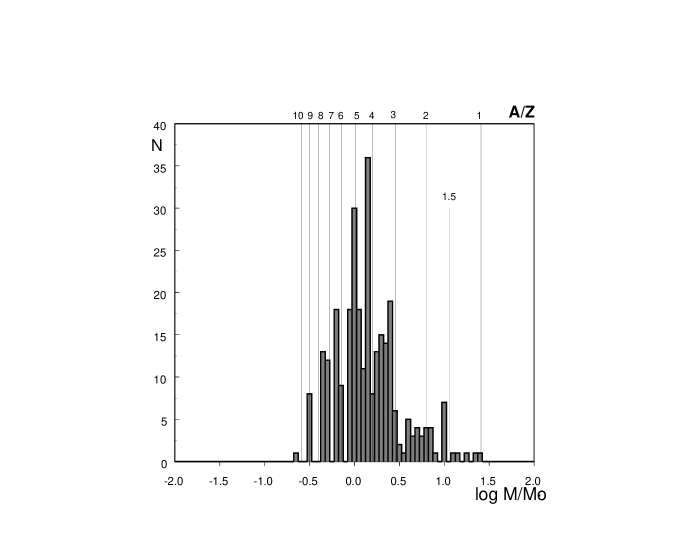
Figure 5.1: The mass distribution of binary stars [7]. On abscissa, the logarithm of the star mass over the Sun mass is shown. Solid lines mark masses, which agree with selected values of A/Z from Eq.(5.26).

Besides, one can see the presence of separate peaks for stars with $A/Z=3;4;5...$ and with $A/Z=3/2$ in Fig.5.1. At that it is important to note, that according to Eq.(5.26) the Sun must consist from a substance with $A/Z=5$. This conclusion is in a good agreement with results of consideration of solar oscillations (Chapter 9).

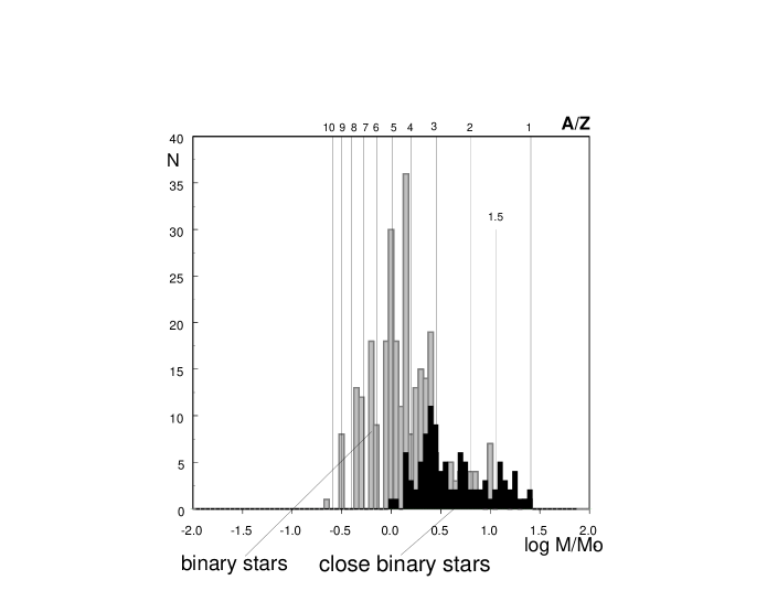
Figure 5.2: The mass distribution of close binary stars [8]. On abscissa, the logarithm of the star mass over the Sun mass is shown. Solid lines mark masses, which agree with selected values of A/Z from Eq.(5.26). The binary star spectrum is shown for comparison.

The mass spectrum of close binary stars is shown in Fig.5.2. It does not contain stars with high parameter $A/Z$, but it is important that both spectra - those of binary stars and those of close binary stars - come abruptly to the end near $A/Z=1$.

5.3.2 Radii of stars

Using Eq.(2.18) and Eq.(5.25), we can determine the star core radius:

$$\mathbb{R}_{\star}=\frac{3(6.84\pi)^{1/3}}{4(Z+1)A/Z}{a_{B}}\left(\frac{\hbar c}{Gm_{p}^{2}}\right)^{1/2}\approx\frac{1.41\cdot 10^{11}}{{(Z+1)A/Z}}cm.$$ (5.27)

The temperature near the star surface is relatively small. It is approximately by 3 orders smaller than it is inside the core. Because of it at calculation of surface parameters, we must take into consideration effects of this order, i.e. it is necessary to take into account the gravity action on the electron gas. At that it is convenient to consider the plasma cell as some neutral quasi-atom (like the Thomas-Fermi atom). Its electron shell is formed by a cloud of free electrons.

Each such quasi-atom is retained on the star surface by its negative potential energy

$$\left(\mathcal{E}_{gravitational}+\mathcal{E}_{electric}\right)<0.$$ (5.28)

The electron cloud of the cell is placed in the volume $\delta V=\frac{4\pi}{3}r_{s}^{3}$, (where $r_{s}\approx\left(\frac{Z}{n_{e}}\right)^{1/3}$) under pressure $P_{e}$. The evaporation of plasma cell releases energy $\mathcal{E}_{PV}=P_{e}V_{s}$, and the balance equation takes the form:

$$\mathcal{E}_{gravitational}+\mathcal{E}_{electric}+\mathcal{E}_{PV}=0.$$ (5.29)

In cold plasma, the electron cloud of the cell has energy $\mathcal{E}_{PV}\approx{e^{2}}{n_{e}}^{1/3}$. in very hot plasma at $kT\gg\frac{Z^{2}e^{2}}{r_{s}}$, this energy is equal to $\mathcal{E}_{PV}=\frac{3}{2}ZkT$. On the star surface these energies are approximately equal:

$$\frac{k\mathbb{T}_{0}}{e^{2}n_{e}^{1/3}}\approx\frac{1}{\alpha}\left(\frac{\mathbb{R}_{0}}{\mathbb{R}_{\star}}\right)^{2}\approx 1.$$ (5.30)

One can show it easily, that in this case

$$\mathcal{E}_{PV}\approx 2Z\sqrt{\frac{3}{2}kT\cdot{e^{2}}{n_{e}}^{1/3}}.$$ (5.31)

And if to take into account Eqs.(4.17)-(4.18), we obtain

$$\mathcal{E}_{PV}\approx 1.5Zk\mathbb{T}_{\star}\left(\frac{\mathbb{R}_{\star}}{\mathbb{R}_{0}}\right)^{3}\sqrt{\alpha\pi}$$ (5.32)

The energy of interaction of a nucleus with its electron cloud does not change at evaporation of the cell and it can be neglected. Thus, for the surface

$$\mathcal{E}_{electric}=\frac{2\pi\mathfrak{P}^{2}}{3n_{s}}=\frac{2G\mathbb{M}_{\star}}{\mathbb{R}_{0}}\left({A}m_{p}-{Z}m_{e}\right).$$ (5.33)

The gravitational energy of the cell on the surface

$$\mathcal{E}_{gravitational}=-\frac{2G\mathbb{M}_{\star}}{\mathbb{R}_{0}}\left({A}m_{p}+{Z}m_{e}\right).$$ (5.34)

Thus, the balance condition Eq.(5.29) on the star surface obtains the form

$$-\frac{4G\mathbb{M_{\star}}Zm_{e}}{\mathbb{R}_{0}}+1.5Zk\mathbb{T}_{\star}\left(\frac{\mathbb{R}_{\star}}{\mathbb{R}_{0}}\right)^{3}\sqrt{\alpha\pi}=0.$$ (5.35)

5.3.3 The ${\mathbb{R}_{\star}}/{\mathbb{R}_{0}}$ ratio and ${\mathbb{R}_{0}}$

With account of Eq.(4.18) and Eqs.(5.24)-(5.23), we can write

$$\frac{\mathbb{R}_{0}}{\mathbb{R}_{\star}}=\left(\frac{\sqrt{\alpha\pi}}{2\beta}\frac{\frac{A}{Z}m_{p}}{m_{e}}\right)^{1/2}\approx{4.56}{\sqrt{\frac{A}{Z}}}$$ (5.36)

As the star core radius is known Eq.(5.27), we can obtain the star surface radius:

$$\mathbb{R}_{0}\approx\frac{6.44\cdot 10^{11}}{(Z+1)(A/Z)^{1/2}}cm$$ (5.37)

5.3.4 The temperature of a star surface

At known Eq.(4.18) and Eq.(5.21), we can calculate the temperature of external surface of a star

$$\mathbb{T}_{0}=\mathbb{T}_{\star}\left(\frac{\mathbb{R}_{\star}}{\mathbb{R}_{0}}\right)^{4}\approx 4.92\cdot 10^{5}\frac{(Z+1)}{(A/Z)^{2}}$$ (5.38)

5.3.5 The comparison with measuring data

The solar oscillations (see Chapter(9)) show that the Sun consists basically from helium-10 with $Z=2,A/Z=5$. With account of this

$$\mathbb{R}_{0}({Z=2,A/Z=5})=9.59\cdot 10^{10}cm,$$ (5.39)

it differs from the measured value of the Sun radius

$$\mathbb{R}_{\odot}=6.96\cdot 10^{10}cm.$$ (5.40)

It can be a consequence of the estimation of the core radius from Eq.(5.27) at $Z=2,A/Z=5$ gives $\mathbb{R}_{\star}(Z=2,A/Z=5)=9.6\cdot 10^{9}cm$, and the ratio of measured radius of the Sun to the calculated value of the core radius is equal

$$\frac{R_{\odot}}{\mathbb{R}_{\star}(Z=2,A/Z=5)}\approx 7.24,$$ (5.41)

where as the calculation Eq.(5.36) gives

$$\frac{\mathbb{R}_{0}}{\mathbb{R}_{\star}(Z=2,A/Z=5)}\approx 10.2$$ (5.42)

At the same time, the calculated value of surface temperature of the Sun (Eq.(5.38)),

$$\mathbb{T}_{0}\approx 5911\,K$$ (5.43)

is in a good agreement with its measured value ($\mathbb{T}_{\odot}\approx 5850\,K$).

The calculation shows that the mass of core of the Sun

$$\mathbb{M}_{\star}(Z=2,A/Z=5)\approx 9.68\cdot 10^{32}~{}g$$ (5.44)

i.t. almost exactly equals to one half of full mass of the Sun

$$\frac{\mathbb{M}_{\star}(Z=2,A/Z=5)}{\mathbb{M}_{\odot}}\approx 0.486$$ (5.45)

in full agreement with Eq.(4.20).

In addition to obtained determinations of the mass of a star Eq.(5.26), its temperature Eq.(5.38) and its radius Eq.(5.37) give possibility to check the calculation, if we compare these results with measuring data. Really, dependencies measured by astronomers can be described by functions:

$$\mathbb{M}=\frac{Const_{1}}{(A/Z)^{2}},$$ (5.46)

$${\mathbb{R}}_{0}=\frac{Const_{2}}{(Z+1)(A/Z)^{1/2}},$$ (5.47)

$${\mathbb{T}}_{0}=\frac{Const_{3}(Z+1)}{(A/Z)^{2}}.$$ (5.48)

If to combine they in the way, to exclude unknown parameter $(Z+1)$, one can obtain relation:

$${\mathbb{T}}_{0}\mathbb{R}_{0}=Const\,\mathbb{M}^{5/4},$$ (5.49)

Its accuracy can by checked. For this checking, let us use the measuring data of parameters of masses, temperatures and radii of close binary stars [8]. The results of these measurements are shown in Fig.(5.3), where the dependence according to Eq.(5.49). It is not difficult to see that these data are well described by the calculated dependence. It speaks about successfulness of our consideration.

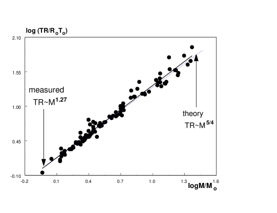
Figure 5.3: The relation between main parameters of stars (Eq.(5.49)) and corresponding data of astronomical measurements for close binary stars [8] are shown.

Chapter 6 The thermodynamic relations of intrastellar plasma

6.1 The thermodynamic relation of star atmosphere parameters

Hot stars steadily generate energy and radiate it from their surfaces. This is non-equilibrium radiation in relation to a star. But it may be a stationary radiation for a star in steady state. Under this condition, the star substance can be considered as an equilibrium. This condition can be considered as quasi-adiabatic, because the interchange of energy between both subsystems - radiation and substance - is stationary and it does not result in a change of a steady state of substance. Therefore at consideration of state of a star atmosphere, one can base it on equilibrium conditions of hot plasma and the ideal gas law for adiabatic condition can be used for it in the first approximation.

It is known, that thermodynamics can help to establish correlation between steady-state parameters of a system. Usually, the thermodynamics considers systems at an equilibrium state with constant temperature, constant particle density and constant pressure over all system. The characteristic feature of the considered system is the existence of equilibrium at the absence of a constant temperature and particle density over atmosphere of a star. To solve this problem, one can introduce averaged pressure

$$\widehat{P}\approx\frac{G\mathbb{M}^{2}}{\mathbb{R}_{0}^{4}},$$ (6.1)

averaged temperature

$$\widehat{T}=\frac{\int_{\mathbb{V}}TdV}{V}\sim\mathbb{T}_{0}\biggl{(}\frac{\mathbb{R}_{0}}{\mathbb{R}_{\star}}\biggr{)}$$ (6.2)

and averaged particle density

$$\widehat{n}\approx\frac{\mathbb{N}_{A}}{\mathbb{R}_{0}^{3}}$$ (6.3)

After it by means of thermodynamical methods, one can find relation between parameters of a star.

6.1.1 The ${c_{P}}/{c_{V}}$ ratio

At a movement of particles according to the theorem of the equidistribution, the energy $kT/2$ falls at each degree of freedom. It gives the heat capacity $c_{v}=3/2k$.

According to the virial theorem [9, 17], the full energy of a star should be equal to its kinetic energy (with opposite sign)(Eq.(5.3)), so as full energy related to one particle

$$\mathcal{E}=-\frac{3}{2}kT$$ (6.4)

In this case the heat capacity at constant volume (per particle over Boltzman constant $k$) by definition is

$$c_{V}=\biggl{(}\frac{dE}{dT}\biggr{)}_{V}=-\frac{3}{2}$$ (6.5)

The negative heat capacity of stellar substance is not surprising. It is a known fact and it is discussed in Landau-Lifshitz course [9]. The own heat capacity of each particle of star substance is positive. One obtains the negative heat capacity at taking into account the gravitational interaction between particles.

By definition the heat capacity of an ideal gas particle at permanent pressure [9] is

$$c_{P}=\biggl{(}\frac{dW}{dT}\biggr{)}_{P},$$ (6.6)

where $W$ is enthalpy of a gas.

As for the ideal gas [9]

$$W-\mathcal{E}=NkT,$$ (6.7)

and the difference between $c_{P}$ and $c_{V}$

$${c_{P}-c_{V}}=1.$$ (6.8)

Thus in the case considered, we have

$$c_{P}=-\frac{1}{2}.$$ (6.9)

Supposing that conditions are close to adiabatic ones, we can use the equation of the Poisson’s adiabat.

6.1.2 The Poisson’s adiabat

The thermodynamical potential of a system consisting of $N$ molecules of ideal gas at temperature $T$ and pressure $P$ can be written as [9]:

$$\Phi=const\cdot N+NTlnP-Nc_{P}TlnT.$$ (6.10)

The entropy of this system

$$S=const\cdot N-NlnP+Nc_{P}lnT.$$ (6.11)

As at adiabatic process, the entropy remains constant

$$-NTlnP+Nc_{P}TlnT=const,$$ (6.12)

we can write the equation for relation of averaged pressure in a system with its volume (The Poisson’s adiabat) [9]:

$$\widehat{P}V^{\widetilde{\gamma}}=const,$$ (6.13)

where $\widetilde{\gamma}=\frac{c_{P}}{c_{V}}$ is the exponent of adiabatic constant. In considered case taking into account of Eqs.(6.6) and (6.5), we obtain

$$\widetilde{\gamma}=\frac{c_{P}}{c_{V}}=\frac{1}{3}.$$ (6.14)

As $V^{1/3}\sim\mathbb{R}_{0}$, we have for equilibrium condition

$$\widehat{P}\mathbb{R}_{0}=const.$$ (6.15)

6.2 The mass-radius ratio

Using Eq.(6.1) from Eq.(6.15), we use the equation for dependence of masses of stars on their radii:

$$\frac{\mathbb{M}^{2}}{\mathbb{R}_{0}^{3}}=const$$ (6.16)

This equation shows the existence of internal constraint of chemical parameters of equilibrium state of a star. Indeed, the substitution of obtained determinations Eq.(5.37) and (5.38)) into Eq.(6.16) gives:

$$(1+Z)\sim(A/Z)^{5/6}$$ (6.17)

Simultaneously the observational data of masses, of radii and their temperatures was obtained by astronomers for close binary stars [8]. The dependence of radii of these stars over these masses is shown in Fig.6.1 on double logarithmic scale. The solid line shows the result of fitting of measurement data $\mathbb{R}_{0}\sim\mathbb{M}^{0.68}$. It is close to theoretical dependence $\mathbb{R}_{0}\sim\mathbb{M}^{2/3}$ (Eq.6.16) which is shown by dotted line.

Figure 6.1: The dependence of radii of stars over the star mass [8]. Here the radius of stars is normalized to the sunny radius, the stars masses are normalized to the mass of the Sum. The data are shown on double logarithmic scale. The solid line shows the result of fitting of measurement data $\mathbb{R}_{0}\sim\mathbb{M}^{0.68}$. The theoretical dependence $\mathbb{R}_{0}\sim\mathbb{M}^{2/3}$ (6.16) is shown by the dotted line.

6.3 The mass-temperature and mass-luminosity relations

Taking into account Eqs.(4.18), (2.22) and (4.8) one can obtain the relation between surface temperature and the radius of a star

$$\mathbb{T}_{0}\sim\mathbb{R}_{0}^{7/8},$$ (6.18)

or accounting for (6.16)

$$\mathbb{T}_{0}\sim\mathbb{M}^{7/12}$$ (6.19)

The dependence of the temperature on the star surface over the star mass of close binary stars [8] is shown in Fig.(6.2). Here the temperatures of stars are normalized to the sunny surface temperature (5875 C), the stars masses are normalized to the mass of the Sum. The data are shown on double logarithmic scale. The solid line shows the result of fitting of measurement data ($\mathbb{T}_{0}\sim\mathbb{M}^{0.59}$). The theoretical dependence $\mathbb{T}_{0}\sim\mathbb{M}^{7/12}$ (Eq.6.19) is shown by dotted line.

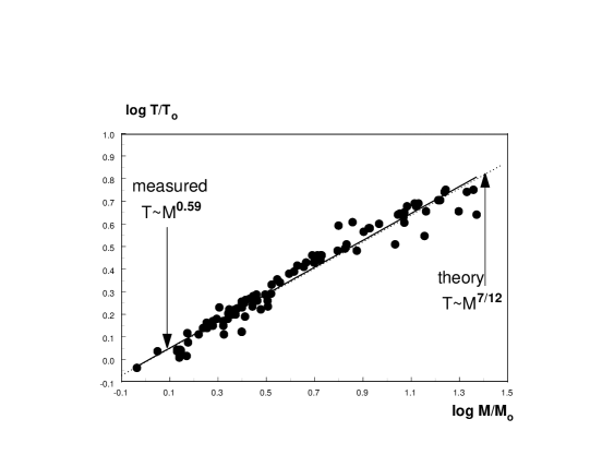
Figure 6.2: The dependence of the temperature on the star surface over the star mass of close binary stars [8]. Here the temperatures of stars are normalized to surface temperature of the Sun (5875 C), the stars masses are normalized to the mass of Sum. The data are shown on double logarithmic scale. The solid line shows the result of fitting of measurement data ($\mathbb{T}_{0}\sim\mathbb{M}^{0.59}$). The theoretical dependence $\mathbb{T}_{0}\sim\mathbb{M}^{7/12}$ (Eq.6.19) is shown by dotted line.

The luminosity of a star

$$\mathbb{L}_{0}\sim\mathbb{R}_{0}^{2}\mathbb{T}_{0}^{4}.$$ (6.20)

at taking into account (Eq.6.16) and (Eq.6.19) can be expressed as

$$\mathbb{L}_{0}\sim\mathbb{M}^{11/3}\sim\mathbb{M}^{3.67}$$ (6.21)

This dependence is shown in Fig.(6.3)

Figure 6.3: The dependence of star luminosity on the star mass of close binary stars [8]. The luminosities are normalized to the luminosity of the Sun, the stars masses are normalized to the mass of the Sum. The data are shown on double logarithmic scale. The solid line shows the result of fitting of measurement data $\mathbb{L}\sim\mathbb{M}^{3.74}$. The theoretical dependence $\mathbb{L}\sim\mathbb{M}^{11/3}$ (Eq.6.21) is shown by dotted line.

It can be seen that all calculated interdependencies $\mathbb{R(\mathbb{M})}$,$\mathbb{T(\mathbb{M})}$ and $\mathrm{L(\mathbb{M})}$ show a good qualitative agreement with the measuring data. At that it is important, that the quantitative explanation of mass-luminosity dependence discovered at the beginning of 20th century is obtained.

Chapter 7 Magnetic fields and magnetic moments of stars

7.1 Magnetic moments of celestial bodies

A thin spherical surface with radius $r$ carrying an electric charge $q$ at the rotation around its axis with frequency $\Omega$ obtains the magnetic moment

$${{\boldsymbol{\mathfrak{m}}}}=\frac{r^{2}}{3c}q\boldsymbol{\Omega}.$$ (7.1)

The rotation of a ball charged at density $\varrho(r)$ will induce the magnetic moment

$$\boldsymbol{\mathfrak{\mu}}=\frac{\boldsymbol{\Omega}}{3c}\int_{0}^{R}r^{2}\varrho(r)~{}4\pi r^{2}dr.$$ (7.2)

Thus the positively charged core of a star induces the magnetic moment

$$\boldsymbol{\mathfrak{m}}_{+}=\frac{\sqrt{G}\mathbb{M}_{\star}\mathbb{R}_{\star}^{2}}{5c}\boldsymbol{\Omega}.$$ (7.3)

A negative charge will be concentrated in the star atmosphere. The absolute value of atmospheric charge is equal to the positive charge of a core. As the atmospheric charge is placed near the surface of a star, its magnetic moment will be more than the core magnetic moment. The calculation shows that as a result, the total magnetic moment of the star will have the same order of magnitude as the core but it will be negative:

$$\boldsymbol{\mathfrak{m}}_{\Sigma}\approx-\frac{\sqrt{G}}{c}\mathbb{M}_{\star}\mathbb{R}_{\star}^{2}\boldsymbol{\Omega}.$$ (7.4)

Simultaneously, the torque of a ball with mass $\mathbb{M}$ and radius $\mathbb{R}$ is

$$\boldsymbol{\mathcal{L}}\approx\mathbb{M}_{\star}\mathbb{R}_{\star}^{2}\boldsymbol{\Omega}.$$ (7.5)

As a result, for celestial bodies where the force of their gravity induces the electric polarization according to Eq.(4.2), the giromagnetic ratio will depend on world constants only:

$$\frac{{\boldsymbol{\mathfrak{m}}}_{\Sigma}}{\boldsymbol{\mathcal{L}}}\approx-\frac{\sqrt{G}}{c}.$$ (7.6)

This relation was obtained for the first time by P.M.S.Blackett [3]. He shows that giromagnetic ratios of the Earth, the Sun and the star 78 Vir are really near to $\sqrt{G}/c$.

By now the magnetic fields, masses, radii and velocities of rotation are known for all planets of the Solar system and for a some stars [14]. These measuring data are shown in Fig.(7.1), which is taken from [14]. It is possible to see that these data are in satisfactory agreement with Blackett’s ratio.

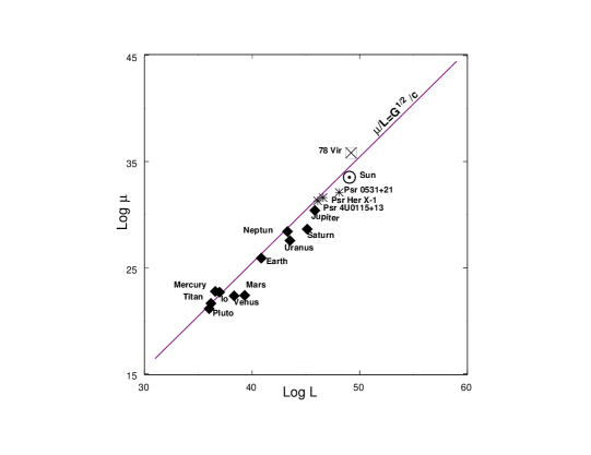
Figure 7.1: The observed values of magnetic moments of celestial bodies vs. their angular momenta [14]. In ordinate, the logarithm of the magnetic moment (in $Gs\cdot{cm^{3}}$) is plotted; in abscissa the logarithm of the angular momentum (in $erg\cdot{s}$) is shown. The solid line illustrates Eq.(7.6). The dash-dotted line fits of observed values.

At some assumption, the same parameters can be calculated for pulsars. All measured masses of pulsars are equal by the order of magnitude [16]. It is in satisfactory agreement with the condition of equilibrium of relativistic matter Eq.(11.12). It gives a possibility to consider that masses and radii of pulsars are determined. According to generally accepted point of view, pulsar radiation is related with its rotation, and it gives their rotation velocity. These assumptions permit to calculate the giromagnetic ratios for three pulsars with known magnetic fields on their poles [2]. It is possible to see from Fig.(7.1), the giromagnetic ratios of these pulsars are in agreement with Blackett’s ratio.

7.2 Magnetic fields of hot stars

To make the above rough estimation for magnetic fields induced by the star atmosphere more accurate, we can take into account the distribution of electric charges inside the star atmosphere In accordance with this distribution, the atmosphere at its rotation induces the moment

$${\boldsymbol{\mathfrak{m}}}_{-}=-\frac{\sqrt{G}\mathbb{M}_{\star}\boldsymbol{\Omega}{\mathbb{R}_{\star}}^{2}}{9c}\int_{\mathbb{R}_{\star}}^{R_{0}}r^{2}\frac{d}{dr}\sqrt{\xi^{3}(2-\xi^{3})}~{}dr,$$ (7.7)

Where $\xi=\frac{\mathbb{R_{\star}}}{r}$.

As $\mathbb{R}_{\star}\ll R_{0}$, the magnetic moment of a core can be neglected. In this case, the total magnetic moment of a star

$${\boldsymbol{\mathfrak{m}}}\approx-2\frac{\sqrt{G}\mathbb{M_{\star}}}{3c}\left(\frac{R_{0}^{7/2}}{\mathbb{R}_{\star}^{3/2}}\right)\boldsymbol{\Omega}.$$ (7.8)

and magnetic field near the pole of a star

$$\boldsymbol{\mathcal{H}}\approx-\frac{2\sqrt{G}\mathbb{M_{\star}}}{9c}\frac{R_{0}^{1/2}}{\mathbb{R}_{\star}^{3/2}}\boldsymbol{\Omega}.$$ (7.9)

Using of substitution of relations obtained above, one can conclude that the magnetic field on a star pole must not depend on the parameter $(Z+1)$ and very slightly depends on $A/Z$, and this dependence can be neglected. I.e. the calculations show that this field practically is not depending on the mass, on the radius and on the temperature of a hot star and must depend on the velocity of star rotation only:

$${\boldsymbol{\mathcal{H}}}\approx-0.47\left(\frac{m_{e}}{m_{p}}\right)^{3/4}\frac{\alpha c}{{G}^{1/2}\beta^{1/4}}{\boldsymbol{\Omega}}\approx-8.8\cdot 10^{8}\boldsymbol{\Omega}{\quad}Oe.$$ (7.10)

The magnetic fields are measured for stars of Ap-class [12]. These stars are characterized by changing their brightness in time. The periods of these changes are measured too. At present there is no full understanding of causes of these visible changes of the luminosity. If these luminosity changes caused by some internal reasons will occur not uniformly on a star surface, one can conclude that the measured period of the luminosity change can depend on star rotation. It is possible to think that at relatively rapid rotation of a star, the period of a visible change of the luminosity can be determined by this rotation in general. To check this suggestion, we can compare the calculated dependence (Eq.7.10) with measuring data [12] (see Fig. 7.2). It can be seen that if magnetic fields of hot stars are really described by the mechanism considered, there are unaccounted factors in this model.

Figure 7.2: The dependence of magnetic fields on poles of Ap-stars as a function of their rotation velocity [12]. The line shows Eq.(7.10)).

It should be said that Eq.(7.10) does not working well in case with the Sun. The Sun surface rotates with period $T\approx 25\div 30$ days. At this velocity of rotation, the magnetic field on the Sun pole calculated accordingly to Eq.(7.10) must be about 1 kOe. The dipole field of Sun according to experts estimation is approximately 20 times lower. There can be several reasons for that.

Chapter 8 The angular velocity of the apsidal rotation in binary stars

8.1 The apsidal rotation of close binary stars

The apsidal rotation (or periastron rotation) of close binary stars is a result of their non-Keplerian movement which originates from the non-spherical form of stars. This non-sphericity has been produced by rotation of stars around their axes or by their mutual tidal effect. The second effect is usually smaller and can be neglected. The first and basic theory of this effect was developed by A.Clairault at the beginning of the XVIII century. Now this effect was measured for approximately 50 double stars. According to Clairault’s theory the velocity of periastron rotation must be approximately 100 times faster if matter is uniformly distributed inside a star. Reversely, it would be absent if all star mass is concentrated in the star center. To reach an agreement between the measurement data and calculations, it is necessary to assume that the density of substance grows in direction to the center of a star and here it runs up to a value which is hundreds times greater than mean density of a star. Just the same mass concentration of the stellar substance is supposed by all standard theories of a star interior. It has been usually considered as a proof of astrophysical models. But it can be considered as a qualitative argument. To obtain a quantitative agreement between theory and measurements, it is necessary to fit parameters of the stellar substance distribution in each case separately.

Let us consider this problem with taking into account the gravity induced electric polarization of plasma in a star. As it was shown above, one half of full mass of a star is concentrated in its plasma core at a permanent density. Therefor, the effect of periastron rotation of close binary stars must be reviewed with the account of a change of forms of these star cores.

According to [4],[13] the ratio of the angular velocity $\omega$ of rotation of periastron which is produced by the rotation of a star around its axis with the angular velocity $\Omega$ is

$$\frac{\omega}{\Omega}=\frac{3}{2}\frac{(I_{A}-I_{C})}{Ma^{2}}$$ (8.1)

where $I_{A}$ and $I_{C}$ are the moments of inertia relatively to principal axes of the ellipsoid. Their difference is

$$I_{A}-I_{C}=\frac{M}{5}(a^{2}-c^{2}),$$ (8.2)

where $a$ and $c$ are the equatorial and polar radii of the star.

Thus we have

$$\frac{\omega}{\Omega}\approx\frac{3}{10}\frac{(a^{2}-c^{2})}{a^{2}}.$$ (8.3)

8.2 The equilibrium form of the core of a rotating star

In the absence of rotation the equilibrium equation of plasma inside star core (Eq.4.4 is

$$\gamma{\bf g}_{G}+\rho_{G}{\bf E}_{G}=0$$ (8.4)

where $\gamma$,${\bf g}_{G}$, $\rho_{G}$ and ${\bf E}_{G}$ are the substance density the acceleration of gravitation, gravity-induced density of charge and intensity of gravity-induced electric field ($div~{}{\bf g}_{G}=4\pi~{}G~{}\gamma$, $div~{}{\bf E}_{G}=4\pi\rho_{G}$ and $\rho_{G}=\sqrt{G}\gamma$).

One can suppose, that at rotation, under action of a rotational acceleration ${\bf g}_{\Omega}$, an additional electric charge with density $\rho_{\Omega}$ and electric field ${\bf E}_{\Omega}$ can exist, and the equilibrium equation obtains the form:

$$(\gamma_{G}+\gamma_{\Omega})({\bf g}_{G}+{\bf g}_{\Omega})=(\rho_{G}+\rho_{\Omega})({\bf E}_{G}+{\bf E}_{\Omega}),$$ (8.5)

where

$$div~{}({\bf E}_{G}+{\bf E}_{\Omega})=4\pi(\rho_{G}+\rho_{\Omega})$$ (8.6)

or

$$div~{}{\bf E}_{\Omega}=4\pi\rho_{\Omega}.$$ (8.7)

We can look for a solution for electric potential in the form

$$\varphi=C_{\Omega}~{}r^{2}(3cos^{2}\theta-1)$$ (8.8)

or in Cartesian coordinates

$$\varphi=C_{\Omega}(3z^{2}-x^{2}-y^{2}-z^{2})$$ (8.9)

where $C_{\Omega}$ is a constant.

Thus

$$E_{x}=2~{}C_{\Omega}~{}x,~{}E_{y}=2~{}C_{\Omega}~{}y,~{}E_{z}=-4~{}C_{\Omega}~{}z$$ (8.10)

and

$$div~{}{\bf E}_{\Omega}=0$$ (8.11)

and we obtain important equations:

$$\rho_{\Omega}=0;$$ (8.12)

$$\gamma g_{\Omega}=\rho{\bf E}_{\Omega}.$$ (8.13)

Since centrifugal force must be contra-balanced by electric force

$$\gamma~{}2\Omega^{2}~{}x=\rho~{}2C_{\Omega}~{}x$$ (8.14)

and

$$C_{\Omega}=\frac{\gamma~{}\Omega^{2}}{\rho}=\frac{\Omega^{2}}{\sqrt{G}}$$ (8.15)

The potential of a positive uniform charged ball is

$$\varphi(r)=\frac{Q}{R}\biggl{(}\frac{3}{2}-\frac{r^{2}}{2R^{2}}\biggr{)}$$ (8.16)

The negative charge on the surface of a sphere induces inside the sphere the potential

$$\varphi(R)=-\frac{Q}{R}$$ (8.17)

where according to Eq.(8.4) $Q=\sqrt{G}M$, and $M$ is the mass of the star.

Thus the total potential inside the considered star is

$$\varphi_{\Sigma}=\frac{\sqrt{G}M}{2R}\biggl{(}1-\frac{r^{2}}{R^{2}}\biggr{)}+\frac{\Omega^{2}}{\sqrt{G}}r^{2}(3cos^{2}\theta-1)$$ (8.18)

Since the electric potential must be equal to zero on the surface of the star, at $r=a$ and $r=c$

$$\varphi_{\Sigma}=0$$ (8.19)

and we obtain the equation which describes the equilibrium form of the core of a rotating star (at $\frac{a^{2}-c^{2}}{a^{2}}\ll 1$)

$$\frac{a^{2}-c^{2}}{a^{2}}\approx\frac{9}{2\pi}\frac{\Omega^{2}}{G\gamma}.$$ (8.20)

8.3 The angular velocity of the apsidal rotation

Taking into account of Eq.(8.20) we have

$$\frac{\omega}{\Omega}\approx\frac{27}{20\pi}\frac{\Omega^{2}}{G\gamma}$$ (8.21)

If both stars of a close pair induce a rotation of periastron, this equation transforms to

$$\frac{\omega}{\Omega}\approx\frac{27}{20\pi}\frac{\Omega^{2}}{G}\biggl{(}\frac{1}{\gamma_{1}}+\frac{1}{\gamma_{2}}\biggr{)},$$ (8.22)

where $\gamma_{1}$ and $\gamma_{2}$ are densities of star cores.

The equilibrium density of star cores is known (Eq.(2.18)):

$$\gamma=\frac{16}{9\pi^{2}}\frac{A}{Z}m_{p}\frac{(Z+1)^{3}}{a_{B}^{3}}.$$ (8.23)

If we introduce the period of ellipsoidal rotation $P=\frac{2\pi}{\Omega}$ and the period of the rotation of periastron $U=\frac{2\pi}{\omega}$, we obtain from Eq.(8.21)

$$\frac{\mathcal{P}}{\mathcal{U}}\biggl{(}\frac{\mathcal{P}}{\mathcal{T}}\biggr{)}^{2}\approx\sum_{1}^{2}\xi_{i},$$ (8.24)

where

$$\mathcal{T}=\sqrt{\frac{243~{}\pi^{3}}{80}}~{}\tau_{0}\approx 10\tau_{0},$$ (8.25)

$$\tau_{0}=\sqrt{\frac{a_{B}^{3}}{G~{}m_{p}}}\approx 7.7\cdot 10^{2}sec$$ (8.26)

and

$$\xi_{i}=\frac{Z_{i}}{A_{i}(Z_{i}+1)^{3}}.$$ (8.27)

8.4 The comparison of the calculated angular velocity of the periastron rotation with observations

Because the substance density (Eq.(8.23)) is depending approximately on the second power of the nuclear charge, the periastron movement of stars consisting of heavy elements will fall out from the observation as it is very slow. Practically the obtained equation (8.24) shows that it is possible to observe the periastron rotation of a star consisting of light elements only.

The value $\xi=Z/[A(Z+1)^{3}]$ is equal to $1/8$ for hydrogen, $0.0625$ for deuterium, $1.85\cdot 10^{-2}$ for helium. The resulting value of the periastron rotation of double stars will be the sum of separate stars rotation. The possible combinations of a couple and their value of $\sum_{1}^{2}\xi_{i}$ for stars consisting of light elements is shown in Table 8.4.

star1	star2	$\xi_{1}+\xi_{2}$
composed of	composed of
H	H	.25
H	D	0.1875
H	He	0.143
H	hn	0.125
D	D	0.125
D	He	0.0815
D	hn	0.0625
He	He	0.037
He	hn	0.0185

Table 8.4

The ”hn” notation in Table 8.4 indicates that the second component of the couple consists of heavy elements or it is a dwarf.

The results of measuring of main parameters for close binary stars are gathered in [8]. For reader convenience, the data of these measurement is applied in the Table in Appendix. One can compare our calculations with data of these measurements. The distribution of close binary stars on value of $(\mathcal{P}/\mathcal{U})(\mathcal{P}/\mathcal{T})^{2}$ is shown in Fig.8.1 on logarithmic scale. The lines mark the values of parameters $\sum_{1}^{2}\xi_{i}$ for different light atoms in accordance with 8.27. It can be seen that calculated values the periastron rotation for stars composed by light elements which is summarized in Table8.4 are in good agreement with separate peaks of measured data. It confirms that our approach to interpretation of this effect is adequate to produce a satisfactory accuracy of estimations.

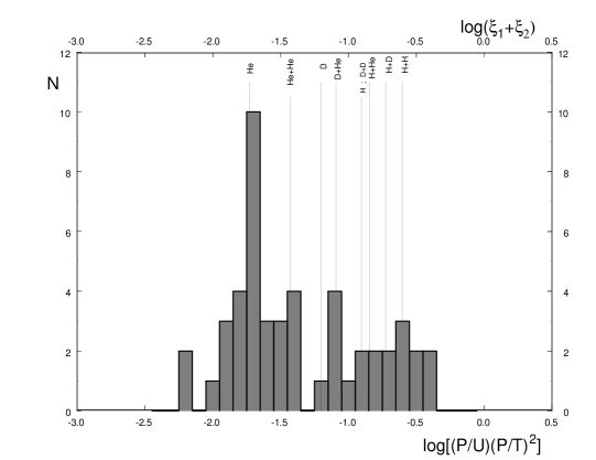
Figure 8.1: The distribution of close binary stars [8] on value of $(\mathcal{P}/\mathcal{U})(\mathcal{P}/\mathcal{T})^{2}$. Lines show parameters $\sum_{1}^{2}\xi_{i}$ for different light atoms in according with 8.27.

Chapter 9 The solar seismical oscillations

9.1 The spectrum of solar seismic oscillations

The measurements [6] show that the Sun surface is subjected to a seismic vibration. The most intensive oscillations have the period about five minutes and the wave length about $10^{4}$km or about hundredth part of the Sun radius. Their spectrum obtained by BISON collaboration is shown in Fig.9.1.

Figure 9.1: $(a)$ The power spectrum of solar oscillation obtained by means of Doppler velocity measurement in light integrated over the solar disk. The data were obtained from the BISON network [6]. $(b)$ An expanded view of a part of frequency range.

It is supposed, that these oscillations are a superposition of a big number of different modes of resonant acoustic vibrations, and that acoustic waves propagate in different trajectories in the interior of the Sun and they have multiple reflection from surface. With these reflections trajectories of same waves can be closed and as a result standing waves are forming.

Specific features of spherical body oscillations are described by the expansion in series on spherical functions. These oscillations can have a different number of wave lengths on the radius of a sphere ($n$) and a different number of wave lengths on its surface which is determined by the $l$-th spherical harmonic. It is accepted to describe the sunny surface oscillation spectrum as the expansion in series [5]:

$$\nu_{nlm}\simeq\Delta\nu_{0}(n+\frac{l}{2}+\epsilon_{0})-l(l+1)D_{0}+m\Delta\nu_{rot}.$$ (9.1)

Where the last item is describing the effect of the Sun rotation and is small. The main contribution is given by the first item which creates a large splitting in the spectrum (Fig.9.1)

$$\triangle\nu=\nu_{n+1,l}-\nu_{n,l}.$$ (9.2)

The small splitting of spectrum (Fig.9.1) depends on the difference

$$\delta\nu_{l}=\nu_{n,l}-\nu_{n-1,l+2}\approx(4l+6)D_{0}.$$ (9.3)

A satisfactory agreement of these estimations and measurement data can be obtained at [5]

$$\Delta\nu_{0}=120~{}\mu Hz,~{}\epsilon_{0}=1.2,~{}D_{0}=1.5~{}\mu Hz,~{}\Delta\nu_{rot}=1\mu Hz.$$ (9.4)

To obtain these values of parameters $\Delta\nu_{0},~{}\epsilon_{0}~{}D_{0}$ from theoretical models is not possible. There are a lot of qualitative and quantitative assumptions used at a model construction and a direct calculation of spectral frequencies transforms into a unresolved complicated problem.

Thus, the current interpretation of the measuring spectrum by the spherical harmonic analysis does not make it clear. It gives no hint to an answer to the question: why oscillations close to hundredth harmonics are really excited and there are no waves near fundamental harmonic?

The measured spectra have a very high resolution (see Fig.(9.1)). It means that an oscillating system has high quality. At this condition, the system must have oscillation on a fundamental frequency. Some peculiar mechanism must exist to force a system to oscillate on a high harmonic. The current explanation does not clarify it.

It is important, that now the solar oscillations are measured by means of two different methods. The solar oscillation spectra which was obtained on program ”BISON”, is shown on Fig.(9.1)). It has a very high resolution, but (accordingly to the Liouville’s theorem) it was obtained with some loss of luminosity, and as a result not all lines are well statistically worked.

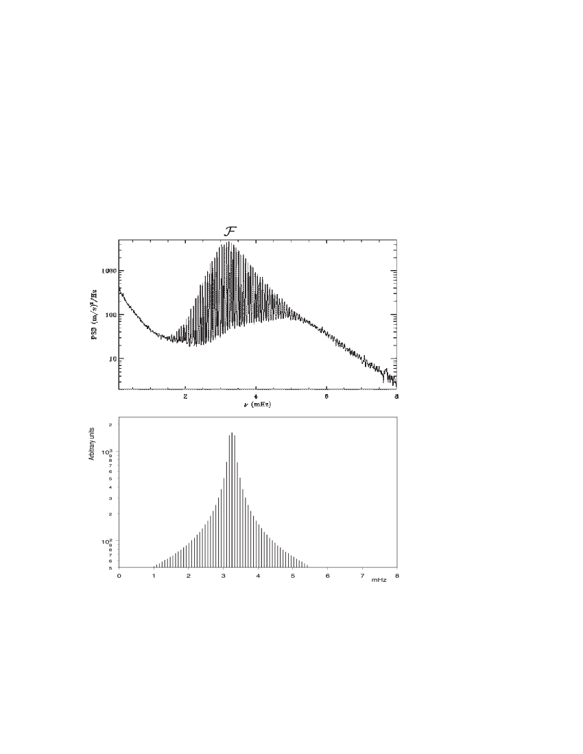
Figure 9.2: $(a)$ The measured power spectrum of solar oscillation. The data were obtained from the SOHO/GOLF measurement [15]. $(b)$ The calculated spectrum described by Eq.(9.26) at $Z=2$ and $A/Z=5$.

Another spectrum was obtained in the program ”SOHO/GOLF”. Conversely, it is not characterized by high resolution, instead it gives information about general character of the solar oscillation spectrum (Fig.9.2)).

The existence of this spectrum requires to change the view at all problems of solar oscillations. The theoretical explanation of this spectrum must give answers at least to four questions :

1.Why does the whole spectrum consist from a large number of equidistant spectral lines?

2.Why does the central frequency of this spectrum ${\cal F}$ is approximately equal to $\approx 3.23~{}mHz$?

3. Why does this spectrum splitting $f$ is approximately equal to $67.5~{}\mu Hz$?

4. Why does the intensity of spectral lines decrease from the central line to the periphery?

The answers to these questions can be obtained if we take into account electric polarization of a solar core.

The description of measured spectra by means of spherical analysis does not make clear of the physical meaning of this procedure. The reason of difficulties lies in attempt to consider the oscillations of a Sun as a whole. At existing dividing of a star into core and atmosphere, it is easy to understand that the core oscillation must form a measured spectrum. The fundamental mode of this oscillation must be determined by its spherical mode when the Sun radius oscillates without changing of the spherical form of the core. It gives a most low-lying mode with frequency:

$$\Omega_{s}\approx\frac{c_{s}}{\mathbb{R}_{\star}},$$ (9.5)

where $c_{s}$ is sound velocity in the core.

It is not difficult to obtain the numerical estimation of this frequency by order of magnitude. Supposing that the sound velocity in dense matter is $10^{7}cm/c$ and radius is close to $\frac{1}{10}$ of external radius of a star, i.e. about $10^{10}cm$, one can obtain as a result

$$F_{s}=\frac{\Omega_{s}}{2\pi}\approx 10^{-3}Hz$$ (9.6)

It gives possibility to conclude that this estimation is in agreement with measured frequencies. Let us consider this mechanism in more detail.

9.2 The sound speed in hot plasma

The pressure of high temperature plasma is a sum of the plasma pressure (ideal gas pressure) and the pressure of black radiation:

$$P=n_{e}kT+\frac{\pi^{2}}{45\hbar^{3}c^{3}}(kT)^{4}.$$ (9.7)

and its entropy is

$$S=\frac{1}{\frac{A}{Z}m_{p}}~{}ln~{}\frac{(kT)^{3/2}}{n_{e}}+\frac{4\pi^{2}}{45\hbar^{3}c^{3}n_{e}}(kT)^{3},$$ (9.8)

The sound speed $c_{s}$ can be expressed by Jacobian [9]:

$$c_{s}^{2}=\frac{D(P,S)}{D(\rho,S)}=\frac{\biggl{(}\frac{D(P,S)}{D(n_{e},T)}\biggr{)}}{\biggl{(}\frac{D(\rho,S)}{D(n_{e},T)}\biggr{)}}$$ (9.9)

or

$$c_{s}=\biggl{\{}\frac{5}{3}\frac{k{T}}{A/Zm_{p}}\biggl{[}1+\frac{2\left(\frac{4\pi^{2}}{45\hbar^{3}c^{3}}\right)^{2}(kT)^{6}}{5n_{e}[n_{e}+\frac{8\pi^{2}}{45\hbar^{3}c^{3}}(kT)^{3}]}\biggr{]}\biggr{\}}^{1/2}$$ (9.10)

For $T={\mathbb{T}_{\star}}$ and $n_{e}=n_{\star}$ we have:

$${\frac{4\pi^{2}(k{\mathbb{T}_{\star}})^{3}}{45\hbar^{3}c^{3}n_{\star}}}=\approx 0.58~{}.$$ (9.11)

Finally we obtain:

$$c_{s}=\biggl{\{}\frac{5}{3}\frac{\mathbb{T}_{\star}}{(A/Z)m_{p}}[1.085]\biggr{)}^{1/2}\approx 5.63~{}10^{7}~{}\biggl{(}\frac{Z+1}{A/Z}\biggr{)}^{1/2}~{}cm/s~{}.$$ (9.12)

9.3 The basic elastic oscillation of a spherical core

Star cores consist of dense high temperature plasma which is a compressible matter. The basic mode of elastic vibrations of a spherical core is related with its radius oscillation. For the description of this type of oscillation, the potential $\phi$ of displacement velocities $v_{r}=\frac{\partial\psi}{\partial r}$ can be introduced and the motion equation can be reduced to the wave equation expressed through $\phi$ [9]:

$$c_{s}^{2}\Delta\phi=\ddot{\phi},$$ (9.13)

and a spherical derivative for periodical in time oscillations $(\sim e^{-i\Omega_{s}t})$ is:

$$\Delta\phi=\frac{1}{r^{2}}\frac{\partial}{\partial r}\biggl{(}r^{2}\frac{\partial\phi}{\partial r}\biggr{)}=-\frac{\Omega_{s}^{2}}{c_{s}^{2}}\phi~{}.$$ (9.14)

It has the finite solution for the full core volume including its center

$$\phi=\frac{A}{r}sin\frac{\Omega_{s}r}{c_{s}},$$ (9.15)

where $A$ is a constant. For small oscillations, when displacements on the surface $u_{R}$ are small $(u_{R}/R=v_{R}/\Omega_{s}R\rightarrow 0)$ we obtain the equation:

$$tg\frac{\Omega_{s}{\mathbb{R}}}{c_{s}}=\frac{\Omega_{s}{\mathbb{R}}}{c_{s}}$$ (9.16)

which has the solution:

$$\frac{\Omega_{s}{\mathbb{R}}}{c_{s}}\approx 4.49.$$ (9.17)

Taking into account Eq.(9.12)), the main frequency of the core radial elastic oscillation is

$$\Omega_{s}=4.49\biggl{\{}\frac{10.85}{(3/2)^{7}\pi}\biggl{[}\frac{Gm_{p}}{r_{B}^{3}}\biggr{]}\frac{A}{Z}\biggl{(}Z+1\biggr{)}^{3}\biggr{\}}^{1/2}.$$ (9.18)

It can be seen that this frequency depends on ${Z}$ and ${A}/{Z}$ only.

Some values of frequencies of radial sound oscillations ${\cal F}=\Omega_{s}/2\pi$ calculated from this equation for selected $A/Z$ at $Z=1$ and $Z=2$ are shown in third column of Table (9.3).

Table(9.3).

		${\cal F},mHz$		${\cal F},mHz$
Z	A/Z	(calculated	star
		on Eq.(9.18))		measured
1	1	0.79	$\eta~{}Bootis$	0.85
			The Procion$(A\alpha~{}CMi)$	1.04
1	2	1.11
			$\beta~{}Hydri$	1.08
2	2	2.03
2	3	2.48	$\alpha~{}Cen~{}A$	2.37
2	4	2.87
2	5	3.24	The Sun	3.23

The measured frequencies of surface vibrations for some stars [5] are shown in right part of this table. The data for $\nu~{}Indus$ and $\xi~{}Hydrae$ also exist [5], but characteristic frequencies of these stars are below 0.3 mHz and they have some other mechanism of excitation, probably. One can conclude from the data of Table 1 that the core of the Sun is basically composed by helium-10. It is not a confusing conclusion, because pressure which exists inside the solar core amounts to $10^{19}{dyne}/{sm^{2}}$ and it is capable to induce the neutronization process in plasma and to stabilize neutron-excess nuclei.

9.4 The low frequency oscillation of the density of a neutral plasma

Hot plasma has the density ${n_{\star}}$ at its equilibrium state. The local deviations from this state induce processes of density oscillation since plasma tends to return to its steady-state density. If we consider small periodic oscillations of core radius

$$R={\mathbb{R}}+u_{R}\cdot sin~{}\omega_{n_{\star}}t,$$ (9.19)

where a radial displacement of plasma particles is small ($u_{R}\ll{\mathbb{R}}$), the oscillation process of plasma density can be described by the equation

$$\frac{d{\mathcal{E}}}{dR}=\mathbb{M}\ddot{R}~{}.$$ (9.20)

Taking into account

$$\frac{d{\mathcal{E}}}{dR}=\frac{d\mathcal{E}_{plasma}}{dn_{e}}\frac{dn_{e}}{dR}$$ (9.21)

and

$$\frac{3}{8}\pi^{3/2}\mathbb{N}_{e}\frac{e^{3}a_{0}^{3/2}}{(k\mathbb{T})^{1/2}}\frac{n_{\star}}{\mathbb{R}^{2}}=\mathbb{M}\omega_{n_{\star}}^{2}$$ (9.22)

From this we obtain

$$\omega_{n_{\star}}^{2}=\frac{3}{\pi^{1/2}}k{\mathbb{T}}\biggl{(}\frac{e^{2}}{a_{B}k{\mathbb{T}}}\biggr{)}^{3/2}\frac{(1+Z)^{3}}{{\mathbb{R}}^{2}A/Zm_{p}}$$ (9.23)

and finally

$$\omega_{n_{\star}}=\biggl{\{}\frac{2^{8}}{3^{5}}\frac{{\pi}^{1/2}}{{10}^{1/2}}\alpha^{3/2}\biggl{[}\frac{Gm_{p}}{a_{B}^{3}}\biggr{]}\frac{A}{Z}\biggl{[}Z+1\biggr{]}^{4.5}\bigg{\}}^{1/2},$$ (9.24)

where $\alpha=\frac{e^{2}}{\hbar c}$ is the fine structure constant. These low frequency oscillations of neutral plasma density are similar to phonons in solid bodies. At that oscillations with multiple frequencies $k\omega_{n_{\star}}$ can exist. Their power is proportional to $1/{\kappa}$, as the occupancy these levels in energy spectrum must be reversely proportional to their energy $k\hbar\omega_{n_{\star}}$. As result, low frequency oscillations of plasma density constitute set of vibrations

$$\sum_{\kappa=1}\frac{1}{\kappa}~{}sin(\kappa\omega_{n_{\star}}t)~{}.$$ (9.25)

9.5 The spectrum of solar core oscillations

The set of the low frequency oscillations with $\omega_{\eta}$ can be induced by sound oscillations with $\Omega_{s}$. At that, displacements obtain the spectrum:

$$u_{R}\sim\sin~{}\Omega_{s}t\cdot\sum_{\kappa=0}\frac{1}{\kappa}~{}\sin~{}\kappa\omega_{n_{\star}}t\cdot\sim\xi\sin~{}\Omega_{s}t+\sum_{\kappa=1}\frac{1}{\kappa}~{}\sin~{}(\Omega_{s}\pm\kappa\omega_{n_{\star}})t,$$ (9.26)

where $\xi$ is a coefficient $\approx 1$.

This spectrum is shown in Fig.(9.2).

The central frequency of experimentally measured distribution of solar oscillations is approximately equal to (Fig.(9.1))

$${\cal F}_{\odot}\approx 3.23~{}mHz$$ (9.27)

and the experimentally measured frequency splitting in this spectrum is approximately equal to

$${f}_{\odot}\approx 68~{}\mu Hz.$$ (9.28)

A good agreement of the calculated frequencies of basic modes of oscillations (from Eq.(9.18) and Eq.(8.4)) with measurement can be obtained at $Z=2$ and $A/Z=5$:

$${\cal F}_{{}_{{}_{Z=2;\frac{A}{Z}=5}}}=\frac{\Omega_{s}}{2\pi}=3.24~{}mHz;~{}f_{{}_{{}_{Z=2;\frac{A}{Z}=5}}}=\frac{\omega_{n_{\star}}}{2\pi}=68.1~{}\mu Hz.$$ (9.29)

Chapter 10 The energy generation and the time of life of the Sun

Now it is commonly accepted to think that the energy generation in stars is basically caused by thermonuclear reactions of hydrogen-helium cycles. It seems to be valid for heavy stars consisting of hydrogen and helium at ratio $A/Z=1\div 2$. In this part of the star mass spectrum (Fig.5.1), sharp lines are absent (beside one related to He-3, probably). This part of spectrum is rather smeared. But this conception is in contradiction with the fact of an existence of the lined spectrum mass of stars with $A/Z>3$. Reaction of this type must go with a change of relation $A/Z$ of a nuclear fuel and ”smearing” of narrow peaks of the spectrum of star masses during milliards of years. It seems that it is possible to make agreement of the measured lined spectrum of these stars and thermonuclear mechanism of reaction, if we suppose that a basic thermonuclear reaction is

$${{}_{Z}^{A}X}+{{}_{Z}^{A}X}={{}_{2Z}^{2A}X}+\gamma$$ (10.1)

i.e., for example, two nuclei of tritium join up into a helium-6 nucleus:

$${{}_{1}^{3}{H}}+{{}_{1}^{3}H}={{}_{2}^{6}He}+\gamma$$ (10.2)

For Sun, a process of nuclear fusion of two nuclei of hydrogen ${}^{5}_{1}H$ joining into helium ${}^{10}_{2}He$ must be prevailing:

$${{}_{1}^{5}{H}}+{{}_{1}^{5}H}={{}_{2}^{10}He}+\gamma$$ (10.3)

The mass of nucleus hydrogen ${}^{5}_{1}H$ is equal approximately to $5.03954$ a.m.u., the mass of helium ${}^{10}_{2}He$ is equal approximately to $10.0524$ . . . Thus, the energy about $4\cdot 10^{-5}$ erg will be emitted in a single reaction. The full number of nuclei in the star core:

$$\mathbb{N}_{\star}=\frac{\mathbb{M}_{\star}}{\frac{A}{Z}m_{p}}\approx 10^{56}.$$ (10.4)

Now the Sun radiates from its surface $3.86\cdot 10^{33}$ erg/s. Approximately $10^{38}$ reactions during one second can provide for this energy. The question emerges: how much hydrogen is there stored into the Sun now?

The answer can be obtained from the analysis of the solar oscillation frequencies. These measurements give two frequencies. Their theoretical dependencies on chemical parameters $A/Z$ and $Z$ are known from Eqs.(9.18) and (9.23). Using these equations, it is possible to express these two chemical parameters:

$$\langle A/Z\rangle=2.33\cdot 10^{-4}\frac{\pi^{6}\alpha^{3}r_{B}^{3}}{Gm_{p}}\biggl{(}\frac{{\cal F}^{3}}{f_{\eta}^{2}}\biggr{)}^{2},$$ (10.5)

$$\langle Z\rangle=\frac{11.14}{\pi\alpha}\biggl{(}\frac{f}{{\cal F}}\biggr{)}^{4/3}-1.$$ (10.6)

The substitution of numerical values gives

$$\langle A/Z\rangle_{\odot}=5.04~{}.$$ (10.7)

and

$$\langle Z\rangle_{\odot}=1.85$$ (10.8)

The last equation speaks that now the Sun must consist approximately from $85\%$ of ${}_{2}^{10}He$ and $15\%$ of ${}_{1}^{5}H$.

Experts think that approximately for the last 5 milliard years the Sun was shining more or less monotone without catastrophic jumps of radiation.

It is not difficult to estimate, that stockpiles of nuclear fuel ${}_{1}^{5}H$ at a present speed burning must be enough to the Sun for several milliard years ahead.

This consideration extremely radically ”solves” the problem of solar neutrinos. Reactions considered above yield no neutrinos at all. In this connection, the question emerges: is it possible to agree the considered mechanism based on the form of stellar mass spectrum with the measured flux of neutrinos?

Chapter 11 Other stars, their classification and some cosmology

The Schwarzsprung-Rassel diagram is now a generally accepted base for star classification. It seems that a classification based on the EOS of substance may be more justified from physical point of view. It can be emphasized by possibility to determine the number of classes of celestial bodies.

The matter can totally have seven states

The atomic substance at low temperature exists as condensed matter (solid or liquid). At high temperature it transforms into gas phase.

The electron -nuclear plasma can exist in four states. It can be relativistic or non-relativistic. The electron gas of non-relativistic plasma can be degenerate (cold) or non-degenerate (hot). If electron gas of plasma is relativistic, its nuclear subsystem may be cold at low temperature. At very high temperature, the energy of nuclear subsystem can exceed the energy of degeneration of relativistic electrons.

In addition to that a substance can exist as neutron matter with nuclear density in degenerate state.

At present, assumptions about existence of matter at different states, other than the above-named, seem unfounded. Thus, seven possible states of matter show a possibility of classification of celestial bodies in accordance with this dividing.

11.1 The atomic substance

11.1.1 Small bodies

Small celestial bodies - asteroids and satellites of planets - are usually considered as bodies consisting from atomic matter.

11.1.2 Giants

The transformation of atomic matter into plasma can be induced by action of high pressure, high temperature or both these factors. If these factors inside a body are not high enough, atomic substance can transform into gas state. The characteristic property of this celestial body is absence of electric polarization inside it. If temperature of a body is below ionization temperature of atomic substance but higher than its evaporation temperature, the equilibrium equation comes to

$$-\frac{dP}{dr}=\frac{G\gamma}{r^{2}}M_{r}\approx\frac{P}{R}\approx\frac{\gamma}{m_{p}}\frac{kT}{R}.$$ (11.1)

Thus, the radius of the body

$$R\approx\frac{GMm_{p}}{kT}.$$ (11.2)

If its mass $M\approx 10^{33}~{}g$ and temperature at its center $T\approx 10^{5}~{}K$, its radius is $R\approx 10^{2}~{}R_{\odot}$. These proporties are characteristic for giants, where pressure at center is about $P\approx 10^{10}~{}din/cm^{2}$ and it is not enough for substance ionization.

11.2 Plasmas

11.2.1 The non-relativistic non-degenerate plasma. Stars.

Characteristic properties of hot stars consisting of non-relativistic non-degenerate plasma was considered above in detail. Its EOS is ideal gas equation.

11.2.2 Non-relativistic degenerate plasma. Planets.

At cores of large planets, pressures are large enough to transform their substance into plasma. As temperatures are not very high here, it can be supposed, that this plasma can degenerate:

$$T<<T_{F}$$ (11.3)

The pressure which is induced by gravitation must be balanced by pressure of non-relativistic degenerate electron gas

$$\frac{G\mathbb{M}^{2}}{6\mathbb{R}\mathbb{V}}\approx\frac{(3\pi^{2})^{2/3}}{5}\frac{\hbar^{2}}{m_{e}}\biggl{(}\frac{\gamma}{m_{p}A/Z}\biggr{)}^{5/3}$$ (11.4)

It opens a way to estimate the mass of this body:

$$\mathbb{M}\approx\mathbb{M}_{Ch}\biggl{(}\frac{\hbar}{mc}\biggr{)}^{3/2}\biggl{(}\frac{\gamma}{m_{p}}\biggr{)}^{1/2}\frac{6^{3/2}9\pi}{4(A/Z)^{5/2}}$$ (11.5)

At density about $\gamma\approx 1~{}g/cm^{3}$, which is characteristic for large planets, we obtain their masses

$$\mathbb{M}\approx 10^{-3}\frac{\mathbb{M}_{Ch}}{(A/Z)^{5/2}}\approx\frac{4\cdot 10^{30}}{(A/Z)^{5/2}}~{}g$$ (11.6)

Thus, if we suppose that large planets consist of hydrogen (A/Z=1), their masses must not be over $4\cdot 10^{30}g$. It is in agreement with the Jupiter’s mass, the biggest planet of the Sun system.

11.2.3 The cold relativistic substance

An energy of a relativistic fermi-system with volume $V$ can be obtained from the general expression [9]:

$$\mathcal{E}=\frac{Vc}{\pi^{2}\hbar^{3}}\int_{0}^{p_{F}}p^{2}\sqrt{m^{2}c^{2}+p^{2}}dp.$$ (11.7)

At integrating of this expression after subtracting of self-energy of particles, we obtain the kinetic energy of $N$ relativistic particles:

$$\mathcal{E}_{kin}=\frac{3}{8}Nmc^{2}\left[\frac{x(2x^{2}+1)\sqrt{x^{2}+1}-Arcsinh(x)-\frac{8}{3}x^{3}}{x^{3}}\right]$$ (11.8)

where $x=\frac{p_{F}}{mc}$ and density of substance:

$$n=\frac{p_{F}^{3}}{3\pi^{2}\hbar^{3}}=\frac{x^{3}}{3\pi^{2}}\left(\frac{mc}{\hbar}\right)^{3}.$$ (11.9)

The pressure of this system is

$$P=-\left(\frac{d\mathcal{E}_{kin}}{dV}\right)_{S=0}=\frac{mc^{2}}{8\pi^{2}}\left(\frac{mc}{\hbar}\right)^{3}\left[x\left(\frac{2}{3}x^{2}-1\right)\sqrt{x^{2}+1}+Arcsinh(x)\right]$$ (11.10)

For simplicity we can suppose that main part of mass of relativistic star is concentrated into its core and it is uniformly distributed here. In this case we can write the pressure balance equation:

$$\frac{GM^{2}}{2R}=3PV.$$ (11.11)

It permits to estimate the full number of particles into the considered system:

$$N=\left(\frac{\hbar c}{Gm_{p}^{2}}\right)^{3/2}\biggl{(}\frac{3}{4\pi}\biggr{)}^{2}\frac{1}{\pi^{3/2}}\left[\frac{x\left(\frac{2}{3}x^{2}-1\right)\sqrt{x^{2}+1}+Arcsinh(x)}{x^{4}}\right]^{3/2}.$$ (11.12)

Accordingly to the virial theorem:

$$\mathcal{E}_{total}=-\mathcal{E}_{kin}$$ (11.13)

and (11.8), the full energy of a relativistic star

$$\mathcal{E}_{total}\sim-\frac{1}{x^{9}}\left[x(2x^{2}+1)\sqrt{x^{2}+1}-Arcsinh(x)-\frac{8}{3}x^{3}\right]\cdot$$

$$\cdot\left[x\left(\frac{2}{3}x^{2}-1\right)\sqrt{x^{2}+1}+Arcsinh(x)\right]^{3/2}.$$ (11.14)

Because this expression has a minimum at $x\approx 1.35$, a star consisting of relativistic substance must have the equilibrium particle density:

$$n_{\star}\approx 8.3\cdot 10^{-2}\left(\frac{mc}{\hbar}\right)^{3}.$$ (11.15)

The relativistic degenerate plasma. Dwarfs.

The degenerate relativistic plasma has a cold relativistic electron subsystem. Its nuclear subsystem can be non-relativistic. The star consisting of this plasma accordingly to Eq.(11.15) at $m=m_{e}$, must have an energy minimum at electron density $n_{\star}\approx 1.4\cdot 10^{30}$ $particle/cm^{3}$ at a star radius

$$R\approx{10^{-2}R_{\odot}}$$ (11.16)

It is not difficult to see that these densities and radii are characteristic for dwarfs.

The neutron matter. Pulsars.

Dwarfs may be considered as stars where a process of neutronization is just beginning. At a nuclear density, plasma turns into neutron matter.

In accordance with Eq.(11.15) at $m=m_{n}$, a star consisting of neutron matter must have the minimal energy at neutron density $n_{\star}\approx 9\cdot 10^{39}$ $particle/cm^{3}$. As result the masses of neutron stars must be approximately equal to $M_{Ch}$. The measured mass distribution of pulsar composing binary stars [16] is shown on Fig.11.1. It can be considered as a confirmation of the last conclusion.

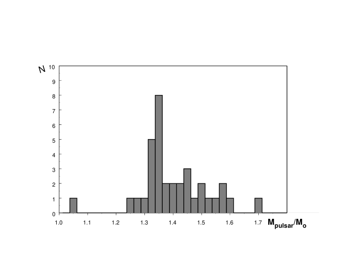
Figure 11.1: The mass distribution of pulsars from binary systems [16].On abscissa the logarithm of pulsar mass in solar mass is shown.

11.2.4 The hot relativistic plasma.Quasars?

Plasma is hot if its temperature is higher than degeneration temperature of its electron gas. The ratio of plasma temperature in the core of a star to the temperature of degradation of its electron gas for case of non-relativistic hot star plasma is (Eq.(2.23))

$$\frac{\mathbb{T}_{\star}}{T_{F}(n_{\star})}\approx 40$$ (11.17)

it can be supposed that the same ratio must be characteristic for the case of a relativistic hot star. At this temperature, the radiation pressure plays a main role and accordingly the equation of the pressure balance takes the form:

$$\frac{GM^{2}}{6RV}\approx\frac{\pi^{2}}{45}\frac{(k\mathbb{T}_{\star})^{4}}{(\hbar c)^{3}}\approx\biggl{(}\frac{\mathbb{T}_{\star}}{T_{F}}\biggr{)}^{3}kTn$$ (11.18)

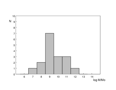
Figure 11.2: The mass distribution of galaxies. [1]. On the abscissa, the logarithm of the galaxy mass over the Sun mass is shown.

This makes it possible to estimate the mass of a hot relativistic star

$$M\approx\biggl{(}\frac{\mathbb{}T_{\star}}{T_{F}}\biggr{)}^{6}\biggl{(}\frac{\hbar c}{Gm_{p}^{2}}\biggr{)}^{3/2}m_{p}\approx 10^{9}M_{\odot}$$ (11.19)

According to the existing knowledge, among compact celestial objects only quasars have masses of this level. Apparently it is an agreed-upon opinion that quasars represent some relatively short stage of evolution of galaxies. If we adhere to this hypothesis, the lack of information about quasar mass distribution can be replaced by the distribution of masses of galaxies [1](Fig.11.2). It can be seen, that this distribution is in a qualitative agreement with supposition that quasars are composed from the relativistic hot plasma.

11.3 Some cosmology

Thus, it seems possible under some assumptions to find characteristic parameters of different classes of stars, if to proceed from EOS of atomic, plasma and neutron substances. Seven EOS can be compared with seven classes of celestial bodies. As any other EOS are unknown, it gives a reason to think that all classes of celestial bodies are discovered. With the exception of ,probably, one body that could have existed in the past. The neutron matter at density of order $10^{40}particle/cm^{3}$ (in accordance with Eq.(11.15)) is not ultra-relativistic matter and its energy and pressure must depend on temperature. It seems, there is no thermodynamical prohibition to imagine this matter so hot when the black radiation pressure will dominate inside it. An estimation shows that it can be possible if mass of this body is near to $10^{50}g$ or even to $10^{55}g$. As it is accepted to think that full mass of the Universe is about $10^{53}g$, it can be assumed that on an early stage of development of Universe, there was some body with a mass about $10^{53}g$ composed by the neutron matter at nuclear density with the radiation at temperature above $10^{12}K$. After some time, with temperature decreased it has lost its stability and decayed into quasars with mass up to $10^{12}M_{Ch}$, consisting of a relativistic plasma with hot nuclear component at $T>10^{10}K$. After next cooling at loosing of stability they was decaying on galaxies of hot stars with mass about $M\approx M_{Ch}$ and core temperature about $T\approx 10^{7}K$, composed by non-relativistic hot plasma. A next cooling must leads hot stars to decaying on dwarfs, pulsars, planets or may be on small bodies. The substances of these bodies (in their cores) consists of degenerate plasma (degenerate electron subsystem and cold nuclear subsystem) or cold neutron matter, it makes them stable in expanding and cooling Universe.

Chapter 12 The conclusion

Evidently, the main conclusion from the above consideration consists in statement of the fact that now there are quite enough measuring data to place the theoretical astrophysics on a reliable foundation. All above measuring data are known for a relatively long time. The traditional system of view based on the Euler equation in the form (1.1) could not give a possibility to explain and even to consider. with due proper attention, to these data. Taking into account the gravity induced electric polarization of plasma and a change starting postulate gives a possibility to obtain results for explanation of measuring data considered above.

Basically these results are the following.

Using the standard method of plasma description leads to the conclusion that at conditions characteristic for the central stellar region, the plasma has the minimum energy at constant density $n_{\star}$ (Eq.(2.18)) and at the constant temperature $\mathbb{T}_{\star}$ (Eq.(5.21)).

This plasma forms the core of a star, where the pressure is constant and gravity action is balanced by the force of the gravity induced by the electric polarization. The virial theorem gives a possibility to calculate the stellar core mass $\mathbb{M}_{\star}$ (Eq.(5.25)) and its radius $\mathbb{R}_{\star}$ (5.27). At that the stellar core volume is approximately equal to 1/1000 part of full volume of a star.

The remaining mass of a star located over the core has a density approximately thousand times smaller and it is convenient to name it a star atmosphere. At using thermodynamical arguments, it is possible to obtain the radial dependence of plasma density inside the atmosphere $n_{a}\approx r^{-6}$ (Eq.(4.17)) and the radial dependence of its temperature $\mathbb{T}_{a}\approx r^{-4}$ (Eq.(4.18)).

It gives a possibility to conclude that the mass of the stellar atmosphere $\mathbb{M}_{a}$ (Eq.(4.19)) is almost exactly equal to the stellar core mass. Thus, the full stellar mass can be calculated. It depends on the ratio of the mass and the charge of nuclei composing the plasma. This claim is in a good agreement with the measuring data of the mass distribution of both - binary stars and close binary stars (Fig. (5.1)-(5.2)). At that it is important that the upper limit of masses of both - binary stars and close binary stars - is in accordance with the calculated value of the mass of the hydrogen star (Eq.(5.26)). The obtained formula explains the origin of sharp peaks of stellar mass distribution - they evidence that the substance of these stars have a certain value of the ratio $A/Z$. In particular the solar plasma according to (Eq.(5.26)) consists of nuclei with $A/Z=5$.

Knowing temperature and substance density on the core and knowning their radial dependencies, it is possible to estimate the surface temperature $\mathbb{T}_{0}$ (5.38) and the radius of a star $\mathbb{R}_{0}$ (5.37). It turns out that these measured parameters must be related to the star mass with the ratio $\mathbb{T}_{0}\mathbb{R}_{0}\sim\mathbb{M}^{5/4}$ (5.49). It is in a good agreement with measuring data (Fig.(5.3)).

Using another thermodynamical relation - the Poisson’s adiabat - gives a way to determine the relation between radii of stars and their masses $\mathbb{R}_{0}^{3}\sim\mathbb{M}^{2}$ (Eq.(6.16)), and between their surface temperatures and masses $\mathbb{T}_{0}\sim\mathbb{M}^{5/7}$ (Eq.(6.19)). It gives the quantitative explanation of the mass-luminosity dependence (Fig.(6.3)).

According to another familiar Blackett’s dependence, the giromagnetic ratios of celestial bodies are approximately equal to $\sqrt{G}/c$. It has a simple explanation too. When there is the gravity induced electric polarization of a substance of a celestial body, its rotation must induce a magnetic field (Fig.(7.1)). It is important that all relatively large celestial bodies - planets, stars, pulsars - obey the Blackett’s dependence. It confirms a consideration that the gravity induced electric polarization must be characterizing for all kind of plasma. The calculation of magnetic fields of hot stars shows that they must be proportional to rotation velocity of stars (7.10). Magnetic fields of Ap-stars are measured, and they can be compared with periods of changing of luminosity of these stars. It is possible that this mechanism is characteristic for stars with rapid rotation (Fig.(7.2)), but obviously there are other unaccounted factors.

Taking into account the gravity induced electric polarization and coming from the Clairault’s theory, we can describe the periastron rotation of binary stars as effect descended from non-spherical forms of star cores. It gives the quantitative explanation of this effect, which is in a good agreement with measuring data (Fig.(8.1)).

The solar oscillations can be considered as elastic vibrations of the solar core. It permits to obtain two basic frequencies of this oscillation: the basic frequency of sound radial oscillation of the core and the frequency of splitting depending on oscillations of substance density near its equilibrium value. It yeils a good agreement with the measuring data and demonstrates that the Sun consists generally of helium-10 (Fig.(9.2)).

A calculation can be carried out in reverse direction. Two measured frequencies of solar oscillations allow to calculate the chemical composition of solar substance. It must be composed by 85% of helium-10 and by 15% of hydrogen-5. It shows that the process of quiet burning of the Sum will be continue for a few milliards years ahead.

The plasma can exists in four possible states. The non-relativistic electron gas of plasma can be degenerate and non-degenerate. Plasma with relativistic electron gas can have a cold and a hot nuclear subsystem. Together with the atomic substance and neutron substance, it gives seven possible states. It suggests a way of a possible classification of celestial bodies. The advantage of this method of classification is in the possibility to estimate theoretically main parameters characterizing the celestial bodies of each class. And these predicted parameters are in agreement with astronomical observations. It can be supposed hypothetically that cosmologic transitions between these classes go in direction of their temperature being lowered. But these suppositions have no formal base at all.

Discussing formulas obtained, which describe star properties, one can note a important moment: these considerations permit to look at this problem from different points of view. On the one hand, the series of conclusions follows from existence of spectrum of star mass (Fig.(5.1)) and from known chemical composition dependence. On the another hand, the calculation of natural frequencies of the solar core gives a different approach to a problem of chemical composition determination. It is important that for the Sun, both these approaches lead to the same conclusion independently and unambiguously. It gives a confidence in reliability of obtained results.

In fact, the calculation of magnetic fields of hot stars only does not give a satisfactory explanation of existing measuring data. At that it is unlikely that the reason of discrepancy is in the use of dubious suggestions - the dipole magnetic field of the Sun is not explained too. But it is important, that the all remaining measuring data (all known of today) confirm both - the new postulate and formulas based on it. At that, the main stellar parameters - masses, radii and temperatures - are expressed through combinations of world constants and at that they show a good accordance with observation data. It is important that quite a satisfactory quantitative agreement of obtained results and measuring data can be achieved by simple and clear physical methods without use of any fitting parameter. It gives a special charm and attractiveness to star physics.

Bibliography

- [1] Allen C.W. - Astrophysical quantities, 1955,University of London, The Athlone Press.
- [2] Beskin V.S., Gurevich A.V., Istomin Ya.N.: Physics of the Pulsar Magnetosphere (Cambridge University Press) (1993)
- [3] Blackett P.M.S.: , 658, (1947)
- [4] Chandrasekhar S.: Monthly Notices of the RAS 93, 449, (1933)
- [5] Christensen-Dalsgaard, J.: Stellar oscillation, Institut for Fysik og Astronomi, Aarhus Universitet, Denmark, (2003)
- [6] Elsworth, Y. at al. - In Proc. GONG’94 Helio- and Astero-seismology from Earth and Space, eds. Ulrich,R.K., Rhodes Jr,E.J. and Däppen,W., Asrtonomical Society of the Pasific Conference Series, vol.76, San Fransisco,76, 51-54.
- [7] Heintz W.D.: Double stars In Geoph. and Astroph. monographs, 15, D.Reidel Publ. Corp., (1978)
- [8] Khaliullin K.F.: Dissertation, Sternberg Astronomical Institute, Moscow, (Russian)(2004) (see Table in Appendix on http://astro07.narod.ru)
- [9] Landau L.D. and Lifshits E.M.: Statistical Physics, 1, 3rd edition, Oxford:Pergamon, (1980)
- [10] Landau L.D. and Lifshits E.M.: Electrodynamics of condensed matter, 1, 3rd edition, Oxford:Pergamon, (1980)
- [11] Leung Y.C.: Physics of Dense Matter In Science Press/World Scientific, Beijing and Singapore, (1984)
- [12] I.I.Romanyuk at al. Magnetic Fields of Chemically Peculiar and Related Stars, Proceedings of the International Conference (Nizhnij Arkhyz, Special Astrophysical Observatory of Russian Academy of Sciences, September 24-27, 1999), eds: Yu. V. Glagolevskij and I.I. Romanyuk, Moscow, 2000, pp. 18-50.
- [13] Russel H.N.: Monthly Notices of the RAS 88, 642, (1928)
- [14] Sirag S.-P.: , 535, (1979)
- [15] Solar Physics, 175/2, (http://sohowww.estec.esa.nl/gallery/GOLF)
- [16] Thorsett S.E. and Chakrabarty D.: E-preprint: astro-ph/9803260, (1998)
- [17] Vasiliev B.V. and Luboshits V.L.: , 345, (1994)
- [18] Vasiliev B.V.: Nuovo Cimento B, 116, pp.617-634, (2001)