Exact analytical expression for the electromagnetic field in a focused laser beam or pulse

Abstract

We present a new class of exact nonsingular solutions for the Maxwell equations in vacuum, which describe the electromagnetic field of the counterpropagating focused laser beams and the subperiod focused laser pulse. These solutions are derived by the use of a modification of the ”complex source method”, investigated and visualized.

1 INTRODUCTION

According to predictions of QED, vacuum can be modified by strong electromagnetic fields if the strength becomes greater than $F_{0}=m^{2}c^{3}/e\hbar=1.32\cdot 10^{16}V/cm$ and, in particular, it should behave as a nonlinear media with respect to transmission of such fields. Different aspects of this phenomenon (including, e.g., vacuum polarization, elastic photon-photon scattering, vacuum birefringence, photon splitting, pair production, etc.) had been investigated theoretically very actively, especially after the beginning of sixties. However, at that time the researchers restricted themselves by considerations of the simplest configurations of the electromagnetic field, namely, a constant homogeneous field and a plane wave field. It was motivated, partially, by simplicity (the Dirac equation in these backgrounds admits exact solutions). But also, it was commonly doubted that the fields with the strength of the order of $F_{0}$ will be really created in a laboratory in viewable times. However, it was declared recently that this experimental task could be handled on the basis of the modern level of technology[1, 2, 3] and moreover, resolution was announced to happen already in the coming decade[2]. The high-intensity field, which can be obtained by implementation of the proposals cited above, will be most probably realized in ultrashort (maybe, subperiod) tightly focused laser pulses of optical range, though alternative projects based on XFEL are also under consideration. Therefore, in order to plan experiments in a near future, one should, firstly, examine whether previous calculations of quantum effects in a strong field can be applied to more realistic fields, and secondly, look for those new effects, which can arise in realistic fields but vanish identically in the homogeneous or the plane wave fields.

In view of this, study of nonlinear QED effects has being risen essentially. Let us mention here just a few of these recent studies, which are most closely related to consideration of the realistic structure of the electromagnetic fields expected in future experiments (for a review of other popular experimental proposals see[4]). In the papers [5, 6, 7] scattering of relativistic electrons on a focused laser beams and pulses was considered. In particular, in [5, 6] the asymmetry of the scattered electrons observed on the experiments was explained. The papers [8, 9] dealt with pair creation from vacuum by a super intense ($E\sim F_{0}$) focused laser pulse or by two colliding pulses. In Refs. [10, 11] a new effect of odd harmonics generation by a tightly focused laser beam in vacuum was investigated. Particularly, it was shown in Refs.[8, 10, 11], that the vacuum quantum effects induced by a tightly focused laser beam or pulse can become observable when the peak strength of the field will reach the values of magnitude of about one order less than the characteristic value $F_{0}$. Another message of these papers was that typically these effects are crucially sensitive to the parameters and the particular type of the model of the field.

However, consideration of the studies mentioned above was based on the approximate model of the focused laser field, which was suggested in Ref. [5] (consideration of Ref. [7] was based on a similar but quite different model which was suggested independently by K. McDonald though not published). This model can be considered as a generalization of the well-known paraxial approximation for a Gaussian beam to the case of a transverse vector field (note, that in Ref. [5] , among the other issues, the classification of polarization types of the focused beam was discussed exhaustively). To take into account finiteness of temporal duration of the pulse, one, roughly speaking, multiplies the carrier field by the slowly varying temporal envelop. It is obvious that this approach is valid only for sufficiently long and weakly focused pulses. In order to check the validity of these approximations, it is desirable to have exact focused beam and pulse-like solutions of the Maxwell equations in vacuum.

Perhaps, the most elegant attempt to construct exact analytical beam or pulse-like field models was made in Refs. [12, 13, 14, 15, 16] for a scalar field and was recently directly generalized to the case of transverse vector fields in Refs. [17, 18]. The main idea of this technique (now called in the literature ”the complex source method”) is to generate the focused fields in vacuum by the pointlike sources whose position is shifted into the complex domain (this is mathematically equivalent to analytical extension of a retarded potential). A first exact analytical model of the focused electromagnetic pulse obtained by this method was manifested in Ref. [18] . Being compared with the approximations described above, this model revealed two new qualitative features. First, the time average of the electric field at any fixed spatial point vanishes identically, which is very reasonable. And second, it possesses some temporal analog of the Gouy phase which provides chirping at the wings of the pulse. This last effect was called in  [18] ”the self-induced blueshift”.

In this paper we show that the usual considerations of this complex source method suffer from two disadvantages. On the one hand, the focused field models presented in the literature thus far[12, 13, 14, 15, 16, 17, 18] possess algebraic singularity, which can be attributed to some real sources (unlike the fictional pointlike ”complex sources”) located on a ring in the focal plane. Therefore, in a sense, these solutions simulate propagation of the focused field through a circular aperture bounded by the branch cut in the focal plane, rather than the field focused in vacuum. Only in the special limiting case of weak focusing (when the paraxial approximation works well) this singularity escapes away to infinity and does not affect the field in the focal spot. On the other hand, as we show below, the complex source method provides analytical solutions only in the form of two colliding beams or pulses (in the limit of weak focusing one of them disappears). We also sketch the method for separating a single pulse solution and discuss the possibility of its representation in a simple analytical form. The consideration below is arranged as follows. In the Sec. 2 we remind how a certain class of electromagnetic field configurations can be parameterized by an axially symmetric scalar field configuration satisfying the usual wave equation. This transformation is very close (in fact, coincides) to the consideration of Ref. [5]. However, in order to increase the clarity of presentation we use different notations and reasoning. Existence of this mapping between the scalar focused fields and a wide class of transverse vector focused fields with clear polarization type (say, circularly polarized e- or h-fields) prevents us from consideration of the more complicated vector version of the ”complex source method”[17, 18]. Therefore, in Sec. 3 we restrict ourselves to the more clear scalar version of the complex source method and demonstrate its drawbacks. The modifications which resolve these problems and the nonsingular beam- and pulse-like solutions of the Maxwell equations are presented in Sec. 4. Our conclusions are collected in Sec. 5.

2 The Narozhny-Fofanov model

Consider a laser beam or pulse focused along the $z$-axis. In the three-dimensional transverse gauge, the electromagnetic field is expressed through the vector potential $\boldsymbol{{\bf A}}$, which satisfies equations

$$\ddot{\boldsymbol{{\bf A}}}-\triangle\boldsymbol{{\bf A}}=0,\quad\nabla\cdot\boldsymbol{{\bf A}}=0.$$ (1)

Let $\rho$, $\phi$ and $z$ be the cylindrical coordinates. Since the pulse is confined in radial direction, the electric and magnetic fields are generally not orthogonal to the direction of propagation of the focused beam or pulse. However, as usually, an arbitrary field can be represented as a superposition of the e-field ($\boldsymbol{{\bf E}}$ orthogonal to $z$) and the h-field ($\boldsymbol{{\bf H}}$ orthogonal to $z$). Since an h-field can be always obtained from the e-field by a duality transformation $\boldsymbol{{\bf E}}\to\boldsymbol{{\bf H}}$, $\boldsymbol{{\bf H}}\to-\boldsymbol{{\bf E}}$, it is enough to consider, say, the case of the e-field. Hence, in the following we assume $A_{z}=0$. In the simplest case of circular polarized field, the pulse consists of photons with $j_{z}=+1$, where $\boldsymbol{{\bf j}}$ is the total angular momentum of the photon (assembled from the orbital momentum $\boldsymbol{{\bf l}}$ and the spin $\boldsymbol{{\bf s}}$). This means, that

$$\frac{1}{i}\frac{\partial\boldsymbol{{\bf A}}}{\partial\phi}+i\,\hat{\boldsymbol{{\bf z}}}\times\boldsymbol{{\bf A}}=\boldsymbol{{\bf A}},$$ (2)

where $\hat{\boldsymbol{{\bf z}}}$ is the unit vector in $z$-direction (compare to discussion of spherical waves in Refs.[19, 20]). The general solution to (2) can be written in the form

$$\boldsymbol{{\bf A}}(\rho,\phi,z,t)=\boldsymbol{{\bf e}}_{+}F_{1}(\rho,z,t)-\boldsymbol{{\bf e}}_{-}F_{2}(\rho,z,t)e^{2i\phi},$$ (3)

where $\boldsymbol{{\bf e}}_{\pm}=\hat{\boldsymbol{{\bf x}}}\pm i\hat{\boldsymbol{{\bf y}}}$, and $F_{1,2}$ – the arbitrary functions (evidently, the latter equation provides decomposition of a state with $j_{z}=l_{z}+s_{z}=+1$ onto the states with $l_{z}=0,\;s_{z}=+1$ and with $l_{z}=+2,\;s_{z}=-1$). By substitution of the anzatz (3) into the equations (2) one obtains the following equations for the auxiliary functions $F_{1,2}$,

$$\triangle F_{1}=\frac{1}{\rho}(\rho F_{1\rho})_{\rho}+F_{1zz}=\ddot{F_{1}},$$ (4)

$$\left(\triangle-\frac{4}{\rho^{2}}F_{2}\right)=\ddot{F_{2}},$$ (5)

$$F_{1\rho}=F_{2\rho}+\frac{2}{\rho}F_{2}.$$ (6)

The electric and magnetic fields can be expressed in terms of functions $F_{1,2}$ by

$$\boldsymbol{{\bf E}}=-\dot{\boldsymbol{{\bf A}}}=-\left(\boldsymbol{{\bf e}}_{+}F_{1t}-\boldsymbol{{\bf e}}_{-}F_{2t}e^{2i\phi}\right),$$ (7)

$$\boldsymbol{{\bf H}}=\nabla\times\boldsymbol{{\bf A}}=-i\left(\boldsymbol{{\bf e}}_{+}F_{1z}+\boldsymbol{{\bf e}}_{-}F_{2z}e^{2i\phi}-2\,\hat{\boldsymbol{{\bf z}}}F_{1\rho}e^{i\phi}\right).$$ (8)

The equations (4), (5) and (6) are compatible and $F_{2}$ can be expressed through $F_{1}$ by

$$F_{2}=F_{1}-\frac{2}{\rho^{2}}\int\limits_{0}^{\rho}F_{1}\rho\,d\rho.$$ (9)

However, it is more suitable to express both functions $F_{1,2}$ in terms of a unique auxiliary function $U(r,z,t)$ through

$$F_{1,2}=U_{\rho\rho}\pm\frac{1}{\rho}U_{\rho},$$ (10)

then the equation (6) is satisfied identically. The new function $U$ obeys just the scalar wave equation

$$\ddot{U}-\triangle U=0,$$ (11)

and it is easy to check that the vector potential can be expressed in the following compact form

$$\boldsymbol{{\bf A}}=2[\boldsymbol{{\bf e}}_{+}\cdot(\hat{\boldsymbol{{\bf z}}}\times\nabla)](\hat{\boldsymbol{{\bf z}}}\times\nabla U).$$ (12)

For example, by choosing an approximate monochromatic solution (i.e., applying a paraxial approximation)

$$U=-\frac{iE_{0}L}{4\omega^{2}(1+2i\chi)}\exp\left(-i\varphi-\frac{\xi^{2}}{1+2i\chi}\right),$$ (13)

for the wave equation (11), where $E_{0}$ is the field strength amplitude, $\xi=\rho/R$, $\chi=z/L$, $R$– the focal radius ($R\gg\lambda=2\pi/\omega$), $L=\omega R^{2}$– the diffractive length, and $\varphi=\omega(t-z)$– the fast phase, one comes to the particular focused beam field model, which was previously proposed by Narozhny and Fofanov and successfully applied to the problems of electron scattering [5, 6], pair creation [8, 9] and harmonics generation [10, 11] by a focused laser field.

In this way it follows that in order to construct a realistic, vector model of the field in a focused electromagnetic beam or pulse, it is sufficient to consider a cylindrically symmetric scalar model first, and then apply the mapping (12). In the next section, let us consider the original complex source method for derivation of scalar focused beam (pulse)-like solutions of the Eq. (11).

3 The complex source method

The idea of the complex source method looks as follows. First, consider a scalar wave equation with an arbitrary variable pointlike source $q(t)$ located at the origin,

$$\ddot{U}-\triangle U=4\pi q(t)\delta(\boldsymbol{{\bf r}}).$$ (14)

Obviously, the created field is expressed in terms of the usual retarded potential,

$$U(\boldsymbol{{\bf r}},t)=\int\limits_{-\infty}^{+\infty}D^{(ret)}(\boldsymbol{{\bf r}},t-t^{\prime})q(t^{\prime})\,dt^{\prime}=\frac{q(t-r)}{r},$$ (15)

where $D^{(ret)}(\boldsymbol{{\bf r}},t)$ is a retarded Green function for the wave equation.

Now, let us shift the location of the source into the complex domain of the $z$ axis, $\boldsymbol{{\bf r}}\to\boldsymbol{{\bf r}}-ib\hat{\boldsymbol{{\bf z}}}$ where $b>0$. It is also suitable to accompany this by a temporal shift $t\to t-ib$. Then, the analytical continuation of the retarded potential (15) reads

$$U(\boldsymbol{{\bf r}},t)=\frac{q(t-ib-{\cal R})}{{\cal R}},\quad{\cal R}^{2}=\rho^{2}+(z-ib)^{2}.$$ (16)

In addition, let us choose the branch of the square root in the definition of ${\cal R}$ so that ${\rm Im}({\cal R})\leq 0$, then in terms of the standard root we have ${\cal R}=(z-ib)\sqrt{1+\rho^{2}/(z-ib)^{2}}$. Then, according to the arguments presented in Refs. [12, 13, 14, 15, 16] , the real part of the field (16) describes a scalar field focused along the $z$ axis and, in particular, satisfies the source free wave equation (11). The viewable meaning of this complex shift transformation can be better understood by consideration in the $\boldsymbol{{\bf k}}$-space. The equation (15) can be represented in the form

$$U_{\boldsymbol{{\bf k}}\omega}=-\frac{4\pi}{(\omega+i0)^{2}-k^{2}}q_{\omega},$$ (17)

and the shift transformation is reduced to $U_{\boldsymbol{{\bf k}}\omega}\to\exp[b(k_{z}-\omega)]U_{\boldsymbol{{\bf k}}\omega}$. On the mass shell, we have $\omega=k$ so that

$$U_{\boldsymbol{{\bf k}}\omega}\to\exp[-b\omega(1-\cos{\theta})]U_{\boldsymbol{{\bf k}}\omega}\approx\exp(-b\omega\theta^{2}/2)U_{\boldsymbol{{\bf k}}\omega},\quad b\gg\lambda$$ (18)

where $\theta$ denotes the angle between ${\bf k}$ and the $z$ axis.

Thus, the complex shift suppresses those wave vectors in Fourier decomposition of the radiated field which are highly inclined with respect to $z$, as it is indeed expected for a focused field. For example, if one chose $q(t)=q_{0}e^{-i\omega t}$ then, in the limit $b\gg\lambda$, $\rho\lesssim(b\lambda)^{1/2}\ll(b^{3}\lambda)^{1/4}$ by applying the expansion ${\cal R}\approx z-ib+\rho^{2}/2(z-ib)$, one can reduce (16) to the form (13) with $L=2b$ and $E_{0}=-8\omega^{2}q_{0}/L^{2}$. On merely these grounds it was proposed in the literature to introduce an additional envelop factor in $q(t)$ and to consider the equation (16) as an exact focused pulse-like solution of the wave equation with the shift parameter $b$ identified with the half of the diffractive length.

Nevertheless, the above arguments are not convincing enough for the following two reasons. First of all, an attempt to consider the Eq. (16) as a solution for the homogeneous wave equation is incorrect and is based on the illusion that the source term in the RHS of the Eq. (14) after the shift, being proportional to $\delta(\boldsymbol{{\bf r}}-ib\hat{\boldsymbol{{\bf z}}})$, should vanish identically when the vector $\boldsymbol{{\bf r}}$ possess real valued components. In fact, a $\delta$–function of a complex argument behaves in a more complicated way than its real argument analog. Presence of the sources follows already from a simple observation that the transformation (18) does not replace the pole singularities in the expression (17) at the mass shell by $\delta(\omega^{2}-k^{2})$. The location of the sources coincides to the ring singularity $\rho=b$, $z=0$ of the expression (16). This ring is picked out physically by zero delay time for radiation emitted by the complex source and crossing the physical hypersurface ${\rm Im}(z)=0$. Moreover, when approaching this singularity along the focal plane $z=0$ we have ${\cal R}\propto\sqrt{|\rho-b|}$, so that $U\propto|\rho-b|^{-1/2}$. This growth is faster than $\log[1/|\rho-b|]$, which could be expected if the linear density of sources was finite at the ring. Since the focal radius $R\sim(b\lambda)^{1/2}$, the singularity becomes safe due to its escape sufficiently far away from the focal region which contains the most part of the field energy only in the weak focusing limit $b\gg\lambda$. However, the paraxial approximation works well exactly in this limit, so that knowledge of the exact solution becomes unnecessary in this case.

Another drawback of the Eq. (16) can be seen from Eq. (18). Indeed, although due to a complex shift the wave vectors with $\theta\gg(b\omega)^{-1/2}$ become suppressed relatively to those with $\theta\lesssim(b\omega)^{-1/2}$, nevertheless they remain be present. The factor $\exp[b(k-k_{z})]$ just mimics but can not replace the true factor $\theta(k_{z})$ which is expected to enter the Fourier decomposition of a single beam or pulse focused along $z$. Therefore, the Eq. (16) actually describes two counterpropagating focused fields of non-commensurable amplitudes. Only in the limit $b\gg\lambda$ the amplitude of a pulse propagating in the direction opposite to $z$ becomes exponentially suppressed.

4 The nonsingular beam and pulse-like solutions

The most obvious and direct way to correct the Eq. (16) and obtain the true, nonsingular solution for Eq. (11) is to take a difference of the retarded and advanced solutions, i.e. to start from

$$U(\boldsymbol{{\bf r}},t)=\int\limits_{-\infty}^{+\infty}\left[D^{(ret)}(\boldsymbol{{\bf r}},t-t^{\prime})-D^{(adv)}(\boldsymbol{{\bf r}},t-t^{\prime})\right]q(t^{\prime})\,dt^{\prime}=\frac{q(t-r)-q(t+r)}{r},$$ (19)

instead of (15). Being a difference between two solutions of the same inhomogeneous equation, the field (19) undoubtedly represents a solution for the corresponding homogeneous, i.e., the wave equation. In particular, (19) is non-singular at the origin (if $q$ is differentiable, of course) and its Fourier transform

$$U_{\boldsymbol{{\bf k}}\omega}=-4\pi\left[\frac{1}{(\omega+i0)^{2}-k^{2}}-\frac{1}{(\omega-i0)^{2}-k^{2}}\right]q_{\omega}=8\pi^{2}i\,{\rm sgn}(\omega)\delta(\omega^{2}-k^{2})q_{\omega}$$

vanishes everywhere except on the mass shell.

Applying the complex shift transformation of the previous section to solution (19), one obtains

$$U(\boldsymbol{{\bf r}},t)=\frac{q(t-ib-{\cal R})-q(t-ib+{\cal R})}{{\cal R}},\quad{\cal R}=\sqrt{\rho^{2}+(z-ib)^{2}},$$ (20)

(since (19) is even with respect to $r$, an arbitrary branch of the square root defining ${\cal R}$ can be chosen in this case).

In order to construct a monochromatic focused beam-like solution, let us choose $q(t)=q_{0}e^{-i\omega t}$, where $q_{0}$ is a normalization constant. Then we have

$$U(\boldsymbol{{\bf r}},t)=2iq_{0}\exp[-\omega b-i\omega t]\frac{\sin(\omega{\cal R})}{{\cal R}}.$$ (21)

Particularly, in paraxial approximation [$b\gg\lambda$, $\rho\lesssim(b\lambda)^{1/2}\ll(b^{3}\lambda)^{1/4}$], by expanding ${\cal R}\backsimeq z-ib+\rho^{2}/2(z-ib)$, we obtain

$$U(\boldsymbol{{\bf r}},t)\backsimeq\frac{iq_{0}}{b(1+iz/b)}\left\{\exp\left[i\omega(z-t)-\frac{\omega\rho^{2}}{2b(1+iz/b)}\right]-\exp\left[-2\omega b-i\omega(z+t)+\frac{\omega\rho^{2}}{2b(1+iz/b)}\right]\right\}.$$

The second term in the parentheses (which had arisen due to a modification proposed here) is exponentially suppressed since $\omega^{-1},\,\rho\ll b$. Therefore, by comparison with Eq. (13), we can identify the parameter $b$ with a half of the diffractive length $L$ and $q_{0}$ with $-E_{0}L^{2}/8\omega^{2}$. In the opposite (formal) case of ultra tight focusing $b\ll\lambda$, our solution (21) reduces to a superposition of smooth convergent and divergent spherical waves, unlike (16), which becomes a convergent spherical wave in the half space $z<0$ and a divergent wave in the half space $z>0$.

The auxiliary functions $F_{1,2}$ introduced in Sec. 2, in the case under consideration read

$$F_{1}=\frac{2iq_{0}\exp[-\omega b-i\omega t]}{{\cal R}^{5}}\left\{\left[2{\cal R}^{2}-3\rho^{2}\right]\left[\omega{\cal R}\cos(\omega{\cal R})-\sin(\omega{\cal R})\right]-\omega^{2}\rho^{2}{\cal R}^{2}\sin(\omega{\cal R})\right\},$$ (22)

$$F_{2}=-\frac{2iq_{0}\exp[-\omega b-i\omega t]}{{\cal R}^{5}}\left\{3\omega{\cal R}\cos(\omega{\cal R})+\left(\omega^{2}{\cal R}^{2}-3\right)\sin(\omega{\cal R})\right\},$$ (23)

and the components of the vector potential and the electric and magnetic fields can be obtained by plugging the expressions (22), (23) into the formulas Eq. (3), (7) and (8) and taking the required derivatives.

As well as the ordinary complex source method, up to now our modification always generates pairs of counterpropagating focused fields. In order to separate out a single focused beam, one can multiply the Fourier transform of the field by the factor $\theta(\pm k_{z})$, which is equivalent to a transformation $U\to U_{\pm}$,

$$U_{\pm}(\rho,z,t)=\pm\frac{1}{2\pi i}\int\limits_{-\infty}^{+\infty}\frac{U(\rho,z^{\prime},t)}{z^{\prime}-z\mp i0}\,dz^{\prime}.$$ (24)

The integral in (24) can be evaluated by enclosing the integration contour and computation of residues if $U$ vanishes at infinite $z$, e.g., if it is given by a rational function. In this particular case, the transformation (24) projects $U$ onto a space of functions which are analytical in the upper half of the complex plane $z$.

Let us discuss in brief application of this transformation to the beam-like solution (21). For this purpose, let us first represent it in a more viewable explicit form

$$U\propto\frac{\exp\left[i\omega(z-ib)\sqrt{1+\frac{\rho^{2}}{(z-ib)^{2}}}\,\right]-\exp\left[-i\omega(z-ib)\sqrt{1+\frac{\rho^{2}}{(z-ib)^{2}}}\,\right]}{(z-ib)\sqrt{1+\frac{\rho^{2}}{(z-ib)^{2}}}}.$$ (25)

For definiteness, in what follows consider extraction of $U_{+}$. After substitution into the formula (24) one obtains two integrals over $z^{\prime}$, each one corresponding to one’s exponent on the RHS of Eq. (25). The first integral can be enclosed in the upper half plane, while the second integral – in the lower one. Furthermore, in the case $\rho<b$ the first integrand in the upper half plane possesses a pole at $z^{\prime}=z+i0$ and the two branch points at $z^{\prime}=i(b\pm\rho)$, while the second one is analytical in the lower half plane. Consequently, $U_{+}$ equals to a contribution in $U$ proportional to the first exponent, added by an additional contribution given by the first integral taken over a closed contour passing around the branch cut connecting the branch points. This correction, however, can not be represented in terms of elementary functions. Similarly, in the case $\rho>b$ the first integrand possesses a pole at $z^{\prime}=z+i0$ and a branch point at $z^{\prime}=i(b+\rho)$, while the second integrand possesses a unique singularity at $z^{\prime}=-i(\rho-b)$. In this case, the branch cuts go from the branch points to imaginary infinity and do not intersect the real axis. Thus, the correction to the contribution in $U$ proportional to the first exponent is given by two integrals over the banks of these cuts. Finally, at the ring $\rho=b$ the second branch point approaches the real axis and $U_{+}$ becomes singular. Therefore, the nonsingular solution (21) is in fact a superposition of two singular counterpropagating beams.

The spatial distributions of the electromagnetic energy density

$$w=\frac{1}{8\pi}\left\{\left[{\rm Re}\,(\boldsymbol{{\bf E}})\right]^{2}+\left[{\rm Re}\,(\boldsymbol{{\bf H}})\right]^{2}\right\},$$ (26)

in the three models of a monochromatic focused beam [the paraxial approximation defined by Eq. (13), the ordinary complex source method defined by Eq. (16), and the modified complex source method defined by Eq. (21)] are compared at the Fig. 1 in the tight focusing regime ($b\sim\lambda$). It is clear from the figure, that in this regime the field model corresponding to the ordinary complex source method occurs to be very close to paraxial approximation (the Narozhny-Fofanov model) everywhere but in the vicinity of the ring singularity, where it breaks down. At the same time, the solution obtained by the modified complex source method, being exact and nonsingular, differs from both of them.

Figure 1: The spatial distribution of the electromagnetic energy density in the monochromatic focused beam: the modified complex source method (curve 1), the complex source method (curve 2) and the paraxial approximation (the Narozhny-Fofanov model, curve 3). Panel (a): Distribution in the focal plane ($z=\phi=0$), panel (b): distribution along the focal axis, and panel (c): distribution along the line parallel to the focal axis and crossing the ring singularity. The values of the parameters used are $b=1$, $q_{0}=1$, $\omega=5$ ($\lambda=1.26$).

The same technique can be applied to construction of the pulse-like solutions as well. In order to do this, it is enough to introduce an envelop factor in $q(t)$, e.g., of the Gaussian form $e^{-t^{2}/2T^{2}}$ or of the Lorentzian form $(1+t^{2}/T^{2})^{-1}$, where $T$ is the duration parameter of the pulse. As it is clear from the consideration above, the result is an expression for the field components in terms of elementary functions, though generally a rather complicated one. Below, let us consider a special but perhaps the most interesting case of an ultrashort, subperiod focused pulse. An especially simple model of a pulse can be obtained if one drops the carrier frequency factor in $q(t)$ totally. Furthermore, since for real values of $t$, $z$ and $\rho$ we have $|{\rm Im}({\cal R})|\leq b$ and hence $-2b\leq{\rm Im}(t-ib\pm{\cal R})\leq 0$, in order to obtain a nonsingular solution for the whole range of the duration parameter, let us choose $q(t)$ to be analytic in the lower half plane of complex $t$. Assuming $q(t)=q_{0}/(1+it/T)$ and applying (20), we have

$$U(\boldsymbol{{\bf r}},t)=\frac{2iq_{0}T}{(T+b+it)^{2}+{\cal R}^{2}}.$$ (27)

The nonsingular solutions corresponding to single pulses propagating along (opposite to) $z$-axis can be extracted from Eq. (27) by using (24) and are given by

$$U_{\pm}(\boldsymbol{{\bf r}},t)=\mp\frac{q_{0}T}{\sqrt{(T+b+it)^{2}+\rho^{2}}\,[z-ib\pm i\sqrt{(T+b+it)^{2}+\rho^{2}}]},$$ (28)

respectively. Thus, unlike the beam-like solution considered above, our solution (27) represents a superposition of two nonsingular counterpropagating focused fields. A more general nonsingular solution of this kind can be constructed as an arbitrary superposition $c_{1}U_{+}(z,\rho,t)+c_{2}U_{+}(z,\rho,-t)$ with complex coefficients. Note also, that in the weak focusing limit $b\to\infty$, $T={\rm const}$, and both expressions (27) and (28) reduce to a plane wave moving along $z$ with the profile $U\backsimeq iq(t-z)/b$.

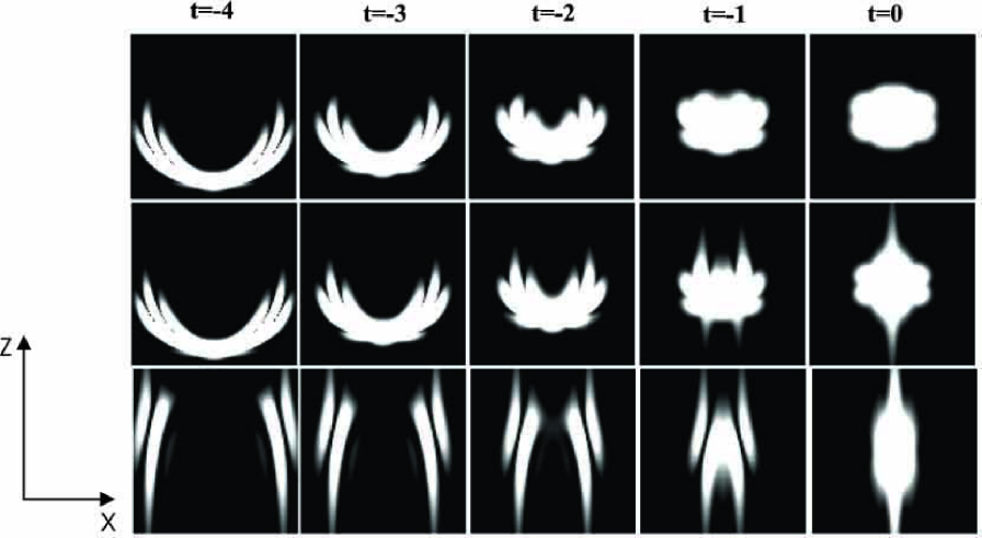
Figure 2: The distribution of the electromagnetic energy density in the $xz$-plane in subsequent stages of focusing of the subperiod pulse-like solutions corresponding to $U$ (the top row), $U_{+}$ (the middle row) and $U_{-}$ (the bottom row). The values of the parameters used are $b=1$, $T=0.2$.

The resulting expressions for the vector potential and the electromagnetic fields are quite cumbersome and this short paper is not an appropriate place to adduce them. Rather, let us present a visualization of the electromagnetic energy distribution in the $xz$-plane, corresponding to Eqs. (27) and (28), at different stages of focusing, see Fig. 2. It can be seen from the pictures, that even in the tight focusing regime $U_{+}$ actually almost coincides to $U$ (i.e., $U_{-}$ is negligible) except for the moments which are directly close to the moment of maximal collapse. Also, it can be recognized that unlike $U$ and $U_{+}$, the backward propagating pulse $U_{-}$ possesses a coreless tubular structure.

In conclusion of the section, let us present an independent derivation of the solution (27) on the basis of direct evaluation of the corresponding Fourier integral. According to the beginning of the section, the Fourier transform to start with is given by

$$U_{\boldsymbol{{\bf k}}\omega}=16\pi^{3}iq_{0}T\theta(\omega)e^{bk_{z}-\omega(T+b)}\delta(\omega^{2}-k_{\perp}^{2}-k_{z}^{2}).$$ (29)

Let us evaluate the Fourier integral $U(\boldsymbol{{\bf r}},t)=\int d\omega\,d^{3}k\,e^{i(\boldsymbol{{\bf k}}\cdot\boldsymbol{{\bf r}}-\omega t)}U_{\boldsymbol{{\bf k}}\omega}/(2\pi)^{4}$ using the cylindrical coordinates in the $k$-space. After performing the integration with respect to the azimuthal angle (which is trivial) and the integration with respect to $k_{z}$ (which is realized by taking away a $\delta$-function), we are left with

$$U(\boldsymbol{{\bf r}},t)=2iq_{0}T\int\limits_{0}^{+\infty}d\omega\,e^{-i\omega(t-ib-iT)}\int\limits_{0}^{\omega}\frac{dk_{\perp}\,k_{\perp}}{\sqrt{\omega^{2}-k_{\perp}^{2}}}\,J_{0}(k_{\perp}\rho)\,\cos\left[(z-ib)\sqrt{\omega^{2}-k_{\perp}^{2}}\right].$$ (30)

The inner integral over $k_{\perp}$ equals[21] $\sin(\omega{\cal R})/{\cal R}$. Hence, the final integral over $\omega$ is elementary and we come to the formula (27). Note that in order to reproduce the Eq. (28) in the same way one should take the integral which is similar to the inner one in (30), but with the imaginary exponent instead of the cosine. However, we could not find it in the mathematical literature thus far.

5 Conclusions

In this paper, we have explicitly demonstrated that the ”complex source method”  [12, 13, 14, 15, 16, 17, 18] of generating the exact focused beam or pulse-like solutions of the wave or Maxwell equations should be modified in order to obtain the fields which are nonsingular in the focal plane, correspondingly to absence of the sources. Also, we have shown that this technique always generates solutions describing a pair of counterpropagating focused fields, rather than a single one. We suggest resolution to both disadvantages. In order to generate nonsingular solutions, one should exploit the difference between the retarded and advanced potentials instead of choosing a special branch of the retarded potential, as it was previously accepted in the literature. Besides, we propose the regular method which allows one to separate the resulting field onto the one propagating along the focal axis and the backward propagating one. However, even if one starts from the nonsingular solution, it is not guaranteed generally that the forward and backward propagating fields will remain nonsingular. Our final proposal is to start with an appropriate anzats for the vector potential in terms of scalar functions obeying the wave equation, and then to construct them by application of the complex source method. This allows one to control the polarization of the electromagnetic field beforehand. A reasonable example of such anzats with known polarization type (e- or h- circularly polarized wave) was proposed in Refs. [5, 6].

As an application of the modified ”complex source method”, we obtained and visualized the solution which describes a counterpropagating focused monochromatic laser beams, and the solution describing a subperiod focused laser pulse. However, the technique under consideration is in no way restricted to the examples given and allows one to obtain a wide class of focused beam- or pulse-like fields. An advantage of this approach is that the field components can be expressed in terms of elementary functions, though generally in a rather complicated way. Nevertheless, it seems that such expressions are very suitable for numerical calculations of both the motion of the charged particles interacting with the laser field and the quantum effects induced by it, especially in the tight focusing regime. The key point for such applications of our expressions is absence of singularities in them.

- [1] B. Shen, and M. Yu, “High-Intensity Laser-Field Amplification between Two Foils,” Phys. Rev. Lett. 89, 275004, 2002.
- [2] T. Tajima, and G. Mourou, “Zettawatt-exawatt lasers and their applications in ultrastrong-field physics,” Phys. Rev. ST Accel. Beams 5, 031301, 2002.
- [3] S. V. Bulanov, T. Esirkepov, and T. Tajima, “Light Intensification towards the Schwinger Limit,” Phys. Rev. Lett. 91, 085001, 2003.
- [4] M. Marklund, and P. K. Shukla, “Nonlinear collective effects in photon-photon and photon-plasma interactions,” Rev. Mod. Phys. 78, 2006.
- [5] N. B. Narozhny, and M. S. Fofanov, “Scattering of Relativistic Electrons by a Focused Laser Pulse,” JETP 90, pp. 753-768, 2000.
- [6] N. B. Narozhny, and M. S. Fofanov, “Anisotropy of electrons accelerated by a high-intensity laser pulse,” Phys. Lett. A 295, pp. 87-91, 2002.
- [7] Yo. I. Salamin, G. R. Mocken, and C. H. Keitel, “Electron scattering and acceleration by a tightly focused laser beam,” Phys. Rev. ST Accel. Beams 5, 101301, 2002.
- [8] N. B. Narozhny, S. S. Bulanov, V. D. Mur, and V. S. Popov, “-pair production by a focused laser pulse in vacuum,” Phys. Lett. A 330, pp. 1-6, 2004.
- [9] N. B. Narozhny, S. S. Bulanov, V. D. Mur, and V. S. Popov, “On pair production by colliding electromagnetic pulses,” JETP Lett. 80, pp. 382-385, 2004.
- [10] A. M. Fedotov, and N. B. Narozhny, “Generation of harmonics by a focused laser beam in the vacuum,” Phys. Lett. A 362, pp. 1-5, 2007.
- [11] N.B. Narozhny, and A.M. Fedotov, “Third harmonic generation in vacuum in the focuse of intense laser beam,” Laser Physics 17, pp. 350-357, 2007.
- [12] G. A. Deschamps, “Gaussian beam as a bundle of complex rays,” Electron. Lett. 7, pp. 684-685, 1971.
- [13] P. D. Einziger, and S. Raz, “Wave solutions under complex space-time shifts,” J. Opt. Soc. Am. A 4, pp. 3-10, 1987.
- [14] E. Heyman, and B. Z. Steinberg, “Spectral analysis of complex-source pulsed beams,” J. Opt. Soc. Am. A 4, pp. 473-480, 1987.
- [15] E. Heyman, and L. B. Felson, “Complex-source pulsed-beam fields,” J. Opt. Soc. Am. A 6, pp. 806-817, 1989.
- [16] R. W. Ziolkowski, “ Localized transmission of electromagnetic energy,” Phys. Rev. A 39, pp. 2005-2033, 1989.
- [17] Zh. Wang, Q. Lin, and Zh. Wang, “Single-cycle electromagnetic pulses produced by oscillating electric dipoles,” Phys. Rev. E 67, 016503, 2003.
- [18] Q. Lin, J. Zheng, and W. Becker, “Subcycle Pulsed Focused Vector Beams,” Phys. Rev. Lett. 97, 253902, 2006.
- [19] W. Heitler, The Quantum Theory of Radiation, Clarendon Press, Oxford, 1954.
- [20] L. D. Landau, E. M. Lifshitz, Quantum electrodynamics, Pergamon Press, New York, 1982.
- [21] I. S. Gradshtein, I. M. Ryzhik, Table of integrals, series, and products, Academic Press, Boston, 1994.