Autowaves in the model of avascular tumour growth

Abstract

A mathematical model of infiltrative tumour growth taking into account cell proliferation, death and motility is considered. The model is formulated in terms of local cell density and nutrient (oxygen) concentration. In the model the rate of cell death depends on the local nutrient level. Thus heterogeneous nutrient distribution in tissue affects tumour structure and development. The existence of automodel solutions is demonstrated and their properties are investigated. The results are compared to the properties of the Kolmogorov-Petrovskii-Piskunov and Fisher equations. Influence of the nutrient distribution on the autowave speed selection as well as on the relaxation to automodel solution is demonstrated. The model adequately describes the data, observed in experiments.

I Introduction

According to experimental data tumour growth can be naturally subdivided into two stages Araujo and McElwain (2004). The initial stage, called avascular growth, is characterized by the tumour consumption of crucial nutrients, such as oxygen or glucose, basically via diffusion. Depending on nutrients concentration tumour cells are supposed to be in one of the three states: proliferating, resting or dead. An avascular tumour is a compact spherically symmetric colony of cancer cells with the necrotic region in the center. Such a rigid structure holds until the tumour size does not exceed several millimeters. Later in response to chemical signals from cancer cells new capillary blood vessels start to grow to provide better nutrients supply. This process, called angiogenesis, indicates the second phase of tumour development – vascular growth.

Although a significant progress in experimental methods has been achieved by now, they still cannot give a conceptual framework within which all the existing data of the tumour development can be fitted Gatenby and Maini (2003). Thereupon the interest in mathematical modelling of the tumour growth and progression has rapidly grown in the last decades. The majority of these models consider avascular tumour growth or growth of multicellular tumour spheroids (MTS) which are prevalent experimental in vitro models of avascular tumours.

There are several basic classes of mathematical models for the avascular tumour or MTS growth. One of them corresponds to “reaction-diffusion type” models which generally consist of an ordinary differential equation for the tumour volume, coupled to one or more parabolic partial-differential equations describing the distribution of nutrients and growth inhibitory factors within the tumour Greenspan (1972); Byrne and Chaplain (1996); Bueno et al. (2005). In models of this type nutrient concentration provides a mitotic and/or death index and the equation for the tumour volume follows from the mass conservation law. Thus, reaction-diffusion models do not consider any cell motion. Also these models can deal only with spherically or cylindrically symmetric spatial structure of a tumour.

In convection-domination models a tumour is considered as incompressible fluid where cell motion is determined by convective velocity field Ward and King (1997); Venkatasubramanian et al. (2006); Tao and Chen (2006). In the models of this type several convection equations describe dynamics of different tumour cell types or phases. Local changes in cell population lead to variations in the internal pressure, which in turn induces motion of tumour cells. These models also include reaction-diffusion equations for spatial nutrient and drug distribution within the tumour. However convection-domination models usually neglect tumour own cell motility. There are rather few models which take into account both convective and random tumour cell motion as well as chemo- or haptotaxis Kolobov et al. (2001, 2003).

For simulation of tumours with large random cell motility Fisher-like equations have usually been used Traqui (1995); Sherratt and Chaplain (2001). In these models a logistic shape for the tumour cell proliferation rate is often used to prevent unlimited growth of local cell density. This rather artificial approach does not take into account nutrient distribution inside the tumour and completly disregards the main cancer property – unlimited growth in the case of a sufficient level of nutrients.

With a rare exception the majority of papers on cancer simulation consider solid tumours as compact objects with the total tumour cell density close to the maximal possible cell density in the tissue. However there is another tumour type, namely infiltrative tumours, for instance glioma, characterized by a rather low value of tumour cell relative density and a large volume of penetration in normal tissue provided by high individual cell motility Chintala and Rao (1996). There are several mathematical models which describe tumours of this type (see, for example, Swanson et al. (2003)). However, spatio-temporal dynamics of nutrients is not taken into account there.

In the present study a 1-D mathematical model for the infiltrative tumour is developed. The model exploits the fact that tumour cell division is possible only in the case of sufficient nutrient concentration. Thus the account of the nutrient spatial distribution effect on the tumour development is the central point of the model considered. The model consists of reaction-diffusion equations for the tumour cell density and nutrient concentration. Dependence of the tumor front propagation rate on the model parameters is obtained both analytically and numerically. Properties of the propagating wave of the dividing tumour cells described by the model are compared to the solution of the Fisher equation.

II The Model

We consider a tumour as a colony of living and dead cells surrounded by normal tissue. Living cells divide with a constant rate and can move in a random way. In the case of nutrients lack tumour cells start to die. We take into account in the model that though a variety of nutrients are necessary for the tumour growth, the oxygen shortage is mostly responsible for the cell death. We consider a tumour growing in a normal tissue with rather poor capillary system, so oxygen diffuse from the blood vessels located sufficiently away from the tumour. Oxygen consumption by normal cells which do not proliferate is neglected as dividing cells consume nutrients much faster than non-proliferating ones. Normal tissue surrounding the tumour is also supposed not to hinder neither cancer cell motion nor proliferation. We restrict our analysis to the case of a single spacial dimension. More formally the model is based on the following physical and biological assumptions

• A tumour grows as a colony of living and dead cells with densities $a$ and $m$ correspondingly.

• Living cells divide with a constant rate $B$ and in the case of low nutrient concentration $s$ starve to death.

• The death rate $P(s)$ depends on the nutrient concentration in a threshold manner which is described below.

• Only random motility (diffusion) with a constant coefficient $D_{a}$ of tumour cells is considered in the model.

• Oxygen is considered as a crucial nutrient for tumour growth. Its distribution is governed by diffusion $D_{s}$ and consumption by the living tumour cells only according to linear law $qa$.

Using these assumptions the governing equations can be written as follows

$$\begin{array}[]{l}\displaystyle\frac{\partial a}{\partial t}=D_{a}\frac{\partial^{2}a}{\partial x^{2}}-P(s)a+Ba,\\ \\ \displaystyle\frac{\partial m}{\partial t}=P(s)a,\\ \\ \displaystyle\frac{\partial s}{\partial t}=D_{s}\frac{\partial^{2}s}{\partial x^{2}}-qa,\end{array}$$ (1)

where $a$, $m$ and $s$ are the proliferating cell density, the dead cell density and the nutrient concentration correspondingly. These equations are written already in a non-dimensional form. In order to estimate the corresponding parameters we take characteristic scales of time and length as $T_{0}=10^{6}$ s and $L=5\cdot 10^{-2}$ cm respectively. The cell density is scaled on $a_{max}=10^{7}$ cells/cm³ (maximal cell density) and the concentration of oxygen in the tissue near blood vessels is supposed to be $S_{max}=10^{-7}$ mol/cm³. In dimensional values the cell proliferation rate corresponds to the cell division frequency of the order of one division per 100 hours. The diffusion coefficients for oxygen and cells are equal to $D_{s}=2.5\cdot 10^{-5}$cm${}^{2}/$s and $D_{a}=2.5\cdot 10^{-9}$ cm${}^{2}/$s respectively. Thus we obtain the following non-dimensional parameters of the problem

$$\begin{array}[]{llllllll}D_{a}=10,&&D_{s}=10^{4},&&B=0.1,&&P_{m}=0.2,\\ S_{crit}=0.3,&&\epsilon=0.01&&q=1.0,\end{array}$$ (2)

which will be referred to as a standard parameter set.

The cell death rate is governed by $P(s)$ which is a step-like function. For $s>S_{crit}$ it is almost equal to zero and for $s<S_{crit}$ it is greater than $B$. We will take it in the form

$$P(s)=P_{m}\displaystyle\frac{1-\tanh[(s-S_{crit})\epsilon]}{2}.$$ (3)

where $P_{m}$ is the maximal value of $P(s)$ and the parameter $\epsilon$ defines the characteristic deviation of $s$ form $S_{crit}$ at which the death rate changes form the values close to zero to the values close to $P_{m}$.

In Eq. (1) the second equation decouples from the rest set. The dead cells density profile determines the position of necrotic region inside the tumour. Therefore it does not affect the tumour spreading, which is governed only by the dynamics of proliferating cells and nutrient concentration and thus Eq. (1) is reduced to the following equations

$$\begin{array}[]{l}\displaystyle\frac{\partial a}{\partial t}=D_{a}\frac{\partial^{2}a}{\partial x^{2}}-P(s)a+Ba,\\ \\ \displaystyle\frac{\partial s}{\partial t}=D_{s}\frac{\partial^{2}s}{\partial x^{2}}-qa.\end{array}$$ (4)

At the avascular stage a tumour is supposed to have a spherically symmetric shape. However if the radius of the tumour is much greater than the characteristic scale, for which the distribution of cell density and nutrient concentration change significantly, then a planar geometry can be considered. In view of our assumption that the tumour grows in the tissue where oxygen predominantly diffuses from the blood vessels located far away from the tumour, the set (4) can be solved in an infinite region. Thus we supplement Eq. (4) with the following boundary conditions on $a$ and $s$

$$\begin{array}[]{llllll}\left\{\begin{array}[]{l}a=0,\\ s_{x}=0\end{array}\right.&\text{for}&x\rightarrow-\infty,&\left\{\begin{array}[]{lll}a=0,\\ s=S_{max}\end{array}\right.&\text{for}&x\rightarrow+\infty.\end{array}$$ (5)

Undoubtedly, any mathematical model of a biological system depends crucially on the choice of parameter values. The parameters vary drastically depending on tumour type, localization, progression etc. The choice of parameters in the model is determined by our objective which is rather a qualitative description of an infiltrative tumour, but not a quantitative description of any specific tumor. Therefore the parameter values are taken in the experimentally observable range and they are not related to a certain kind of cancer. The other important limitation on parameters is that their values are chosen in such a way that the tumour cell density remains substantially smaller than the maximal value, which is typical for an infiltrative type of a tumour.

III Travelling wave solutions

We seek the solution to Eq. (4) in the form of a wave travelling with a constant shape and speed $c$ (i.e. an autowave). Then the governing equations (4) are reduced to a set of ordinary differential equations by introducing the automodel coordinate frame $\xi=x-ct$

$$\begin{array}[]{l}\displaystyle D_{a}\frac{\partial^{2}a}{\partial\xi^{2}}+c\frac{\partial a}{\partial\xi}-P(s)a+Ba=0,\\ \\ \displaystyle D_{s}\frac{\partial^{2}s}{\partial\xi^{2}}+c\frac{\partial s}{\partial\xi}-qa=0\end{array}$$ (6)

with the following boundary conditions

$$\begin{array}[]{llllll}\left\{\begin{array}[]{l}a=0,\\ s=\sigma\end{array}\right.&\text{for}&\xi\rightarrow-\infty,&\left\{\begin{array}[]{lll}a=0,\\ s=1\end{array}\right.&\text{for}&\xi\rightarrow+\infty.\end{array}$$ (7)

Here the constant $\sigma$ corresponds to the limiting constant value of the substrate concentration on $-\infty$. We refer to the parameters $c$ and $\sigma$ as internal parameters contrary to the control parameters, listed in (2). On the first step we consider the asymptotic behavior of the solutions of Eq. (6) on $\xi=\pm\infty$. In order to do this we linearize Eq. (6) near the values (7) which are stationary points of (6) and obtain two sets of ODEs with constant coefficients

$$\begin{array}[]{l}\displaystyle D_{a}\frac{\partial^{2}a^{-}}{\partial\xi^{2}}+c\frac{\partial a^{-}}{\partial\xi}(B-P(\sigma))a^{-}=0,\\ \\ \displaystyle D_{s}\frac{\partial^{2}s^{-}}{\partial\xi^{2}}+c\frac{\partial s^{-}}{\partial\xi}-qa^{-}=0,\end{array}$$ (8)

and

$$\begin{array}[]{l}\displaystyle D_{a}\frac{\partial^{2}a^{+}}{\partial\xi^{2}}+c\frac{\partial a^{+}}{\partial\xi}Ba^{+}=0,\\ \\ \displaystyle D_{s}\frac{\partial^{2}s^{+}}{\partial\xi^{2}}+c\frac{\partial s^{+}}{\partial\xi}-qa^{+}=0.\end{array}$$ (9)

According to linear differential calculus the solutions to these problems are sought in the form $(a,~{}a_{\xi},~{}s,~{}s_{\xi})^{T}\sim{\bf k}^{\pm}\exp(\mu^{\pm}\xi)$ which reduces the systems of linear differential equations to eigenvalue problems for coefficients $\mu^{\pm}$ as eigenvalues and constant vectors ${\bf k}^{\pm}$ as eigenvectors. Eigenvalues $\mu^{\pm}$ indicate the rate of exponential convergence (divergence) of the solutions to the boundary values (7) as $\xi\rightarrow\pm\infty$ and superscripts ‘+’ and ‘-’ refer to the linearized problem on $+\infty$ and $-\infty$ respectively.

For the case $\xi\rightarrow-\infty$ it appears that the linearized set of ODEs (8) has a singe solution with the rate of exponential convergence to the boundary conditions given by $\mu^{-}_{1}=(-c+\sqrt{c^{2}+4(P(\sigma)-B)D_{a}})/2D_{a}$, two solutions unbounded for $\xi\rightarrow-\infty$ with the rates of exponential divergence $\mu^{-}_{2}=(-c-\sqrt{c^{2}+4(P(\sigma)-B)D_{a}})/2D_{a}$, $\mu^{-}_{3}=-c/D_{s}$, and a single solution with a zero coefficient, $\mu^{-}_{4}=0$, of exponential growth. It can be shown that the stationary point $\{S1:a=0,s=\sigma\}$ of (6) is either a saddle-node if $\mu^{-}_{1}$ is real positive, a stable node if $\mu^{-}_{1}$ is real negative, or a stable focus if $\mu^{-}_{1}$ is a complex number.

In the same manner, for the case $\xi\rightarrow+\infty$ we derive the set of ODEs (9) linearized near the boundary conditions (7) which has four linearly independent solutions bounded for $\xi\rightarrow+\infty$ and characterized by the rates of exponential convergence $\mu_{1,2}^{+}=(-c\pm\sqrt{c^{2}-4BD_{a}})/2D_{a}$, $\mu^{+}_{3}=-c/D_{s}$, $\mu^{+}_{4}=0$. A simple consideration shows that the stationary point $\{S2:a=0,s=1\}$ is either a stable node or a stable focus. In the latter case $a$ can become negative and therefore this solution is physically unrealistic.

The eigenvectors associated with the linearized problems can be written as ${\bf k}^{\pm}_{1,2}=(1,~{}\mu^{\pm}_{1,2},q/\Lambda^{\pm}_{1,2},~{}\mu^{\pm}_{1,2}q/\Lambda^{\pm}_{1,2})^{T}$, ${\bf k}^{\pm}_{3}=(0,~{}0,~{}1,\mu^{\pm}_{3})^{T}$ and ${\bf k}^{\pm}_{4}=(0,~{}0,~{}1,~{}0)^{T}$. Here we have introduced a notation $\Lambda^{\pm}_{1,2}=\sqrt{D_{s}\mu^{\pm 2}_{1,2}+c\mu^{\pm}_{1,2}}$.

Taking into account that the solution of Eq. (6,7) exist only if the coefficient $\mu^{-}_{1}$ is a real positive number ($S1$ is a saddle-node) and $\mu^{+}_{1,2,3}$ are real numbers ($S2$ is a stable node) we derive the following restrictions on the model parameters

$$\begin{array}[]{lll}P(\sigma)>B,&&\displaystyle c\geq 2\sqrt{BD_{a}}.\end{array}$$ (10)

The last condition implies that an automodel solution of Eq. (4) can propagate only with the velocity higher or equal to some minimal value $c_{min}=2\sqrt{BD_{a}}$. This property of the set (4) solutions is similar to the one of the KPP (Kolmogorov-Petrovskii-Piskunov) Kolmogorov et al. (1937) equation and its special case, Fisher equation Fisher (1937), which also exhibit autowaves.

The first inequality in (10) shows that since $P(s)$ is a monotonic decreasing function there exist autowaves characterized by the residual concentration of the substrate left behind the travelling wave and this residual concentration is less or equal to some critical value $\sigma_{max}=P^{-1}(B)$, i.e. $\lim_{\xi\rightarrow-\infty}s(\xi)=\sigma\leq\sigma_{max}$. The existence of both the parameter $\sigma$ and the limiting condition makes our model different from the KPP model.

It can be also shown that for the travelling wave solution of Eq. (6) the substrate concentration profile is a monotonic function of the coordinate $\xi$. In order to do this we multiply the second equation in (6) by the integrating factor $exp(c/D_{s}\xi)$ and integrate it over $\xi$ to obtain

$$D_{s}s(\xi)_{\xi}e^{c/D_{s}\xi}=q\int_{-\infty}^{\xi}a(z)e^{c/D_{s}z}dz.$$ (11)

The integral in the right hand side of Eq. (11) is always positive therefore $s_{\xi}$ is positive and $s(\xi)$ is a monotonic growing function.

IV Numerical simulations

We solve Eq. (6) subject to boundary conditions (5) numerically by using shooting and relaxation methods. Here we skip the description of these methods since they can be found in our previous papers (see Gubernov et al. (2003) and references therein). The problem for numerical calculation is posed on a finite domain $\xi\in[-L,L]$, where $L$ is taken to be sufficiently large, with a uniform grid on it. The integration step and $L$ values are chosen in such way that both twice decreasing the integration step and twice increasing the integration interval results in a variation of the calculated parameters (such as wave speed) in the ninth significant digit only.

The stability analysis of autowave solutions travelling with different velocities is studied numerically. Equations (4) are solved in a coordinate frame moving with a minimal speed ($\xi=x-c_{min}t$). The boundary conditions (5) are imposed at the edge points of the space grid. For our numerical algorithm we use the method splitting with respect to physical processes. Initially we solve the set of ODEs which describes the cell birth and death processes as well as nutrient consumption by using the fourth order Runge-Kutta algorithm. As a next step, equations of mass transfer for oxygen and cells are solved with the Crank-Nicolson method of the second order approximation in space and time.

Figure 1: Cell density profile as a function of coordinate $\xi$ in the moving frame (top figure) and projections of phase trajectories onto the plane $(a,~{}a_{\xi})$ (bottom figure) for standard parameter values and various values of the wave speed $c\geq c_{min}$.

Typical solution profiles for the cell density, $a(\xi)$, and a projection of phase trajectories into the plane $(a,~{}a_{\xi})$ are shown in the top and bottom figures 1 respectively for various values of the wave speed $c\geq c_{min}$, where $c_{min}=2\sqrt{2}$ in this case. In the bottom figure 1 we also show the asymptotic behavior of the solutions of Eq. (6-7) for $\xi\rightarrow\pm\infty$ with straight lines which represent the trajectories of problems obtained form Eq. (6) by linearizing it near the boundary conditions (7). The cell density profile looks like a sharp peak so that $a$ vanishes quickly form its maximum value in a relatively thin region of the $\xi$ coordinate. As we increase $c$ the $a(\xi)$ the profile becomes less localized and the maximum value of the cell density $a(0)$ increases as well. It can be shown, however, that $a(0)$ always remains less than one. The substrate concentration profile $s(\xi)$ is a monotonic growing function of coordinate $\xi$ (not shown here for the sake of brevity), which is almost constant, $s(\xi)\sim\sigma$ for $\xi<0$ and exhibits a slow exponential growth to its boundary value ($s=1$ as $\xi\rightarrow\infty$) for $\xi>0$ with the rate of growth $c/D_{s}$. The switching between these two regimes occurs in the thin region near $\xi=0$ where $a$ reaches the maximal value and coupling between the two equations in (6) is strong.

Figure 2: Cell density profile as a function of coordinate $\xi$ in the moving frame (top figure) and projections of phase trajectories onto a plane $(a,~{}a_{\xi})$ (bottom figure) for standard parameter values and various values of speed $c<c_{min}$.

In the top and bottom figures 2 we plot a typical solution profiles for the cell density $a(\xi)$, and a projection of phase trajectories onto the plane $(a,~{}a_{\xi})$ respectively for the several values of speed below the minimal value $c<c_{min}=2$ as shown in figure. In figure 2 it is clearly seen that at certain $\xi$ values cell density becomes negative which is not physically feasible. Therefore we consider the solutions for which $a(\xi)\geq 0$, travelling with the speed higher than or equal to a minimal value $c_{min}$.

As a next step we investigate the dependence of the speed of the autowave solution as a function of parameters of the problem. In the top figure 3 the dependence of $c$ on $\sigma$ is plotted for the physically feasible solutions travelling with the speed higher than $c_{min}$ (we refer to them as monotonic solutions) for standard parameter values and several values of $B$ as shown in Fig. 3. For fixed control parameter values there exists a family of solutions $c(\sigma)$ travelling with different speeds. For each value of $B$ the speed is scaled on the minimal value $c_{min}=2\sqrt{BD_{a}}$, which is also shown with a dotted line marked ”$c=c_{min}$”. All monotonic solution branches cease to exist when $c/c_{min}$ ratio drops down to $1$. Below this value a family of the oscillatory solution (which are not physically feasible) branches emerges. These solutions are plotted in the bottom figure 3 with dashed lines. It is worthwhile noting that at $c/c_{min}=1$ only the second condition in (10) is violated, whereas the first condition is approached along the oscillatory branches when speed of the wave drops down to zero and $\sigma$ reaches maximum which is shown in the bottom figure 3.

Figure 3: Dependence of $c/c_{min}$ on $\sigma$ for various values of $B$.

We use the solutions obtained by solving Eq. (6) as the initial conditions for numerical integration of Eq. (4) subject to boundary conditions (5) in order to investigate the stability of these autowaves. In Fig. 4 we show a spatial-temporal evolution of the initial profiles obtained by numerical integration of Eq. (6) with the speed equal to the minimal value, $c=c_{min}$ (top figure), and with the speed higher than minimum, $c=5$ (bottom figure). The standard parameter values are used to perform this calculation. We use the travelling coordinate frame, $\xi=x-c_{min}t$, so that the solution propagating with the minimal speed is presented in the top figure 4 as a standing wave, whereas the solution corresponding to $c=5$ is shown in the bottom figure 4 as a wave travelling with the speed $c=5-c_{min}$. The set (4) is integrated over the time periods of the order of $t=400B^{-1}$, where $B^{-1}$ is the characteristic time scale for the instability growth in Eq. (4). Results of numerical simulation of Eq. (4) are shown in Fig. 4 for two values of the wave speed and demonstrate that autowaves can propagate stably for long intervals of time without changing their speed and form.

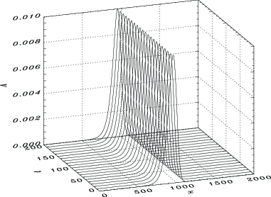
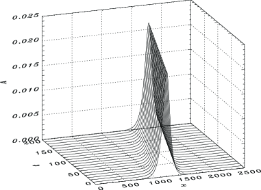
Figure 4: Dependence of cell density, $a$, on coordinate, $\xi$, in the frame travelling with the minimal speed, and on time $t$ for the standard parameter values. Initial profiles correspond to $c=c_{min}$ (top figure) $c=5$ (bottom figure).

V Limit $\epsilon=0$

In the limit $\epsilon\rightarrow 0$ the governing equations (4) allow the following simplifications: (i) the cell death rate function can be replaced by a Heaviside step function $P_{m}H(s-S_{cr})$, (ii) due to translational invariance of Eq. (4) we may require the travelling solution to satisfy the condition $s(\xi)|_{\xi=0}=S_{crit}$. This implies that $P(s(\xi))=0$ for $\xi<0$ and $P(s(\xi))=P_{m}$ for $\xi>0$. In this case Eq. (6) can be considered in two semi-infinite intervals $\xi\in(-\infty,0)$ and $\xi\in(0,\infty)$ separately. This yields a set of ODEs similar to Eq. (8) for $\xi<0$, where $P(\sigma)$ is replaced by $P_{m}$, and a set (9) for $\xi>0$. The unknown functions $a^{\pm}$ and $s^{\pm}$ satisfy the boundary conditions (7) for $\xi\rightarrow\pm\infty$ respectively and can be written explicitly as

$${\bf u}^{\pm}(\xi)=\displaystyle\sum_{i=1}^{4}\alpha^{\pm}_{i}{\bf k}^{\pm}_{i}e^{\mu^{\pm}_{i}\xi},$$ (12)

where ${\bf u}^{\pm}\equiv(a^{\pm},~{}a_{\xi}^{\pm},~{}s^{\pm},~{}s_{\xi}^{\pm})^{T}$; ${\bf k}^{\pm}_{i}$ and $\mu^{\pm}_{i}$ are taken from the section III (where $P(\sigma)$ is replaced by $P_{m}$) and $\alpha^{\pm}_{i}$ are constant coefficients which are to be found. From boundary conditions (7) it follows that $\alpha^{-}_{2}=0$, $\alpha^{-}_{3}=0$, $\alpha^{-}_{4}=\sigma$ and $\alpha^{+}_{4}=1$. The other four constants can be found from continuity conditions across $\xi=0$ for $a(\xi)$: $a^{-}(0)=a^{+}(0)$, $s(\xi)$: $s^{-}(0)=s^{+}(0)$, and $s_{\xi}(\xi)=S_{crit}$: $s_{\xi}^{-}(0)=s_{\xi}^{+}(0)$. This yields four equations

$$\begin{array}[]{l}\alpha^{-}_{1}=\alpha^{+}_{1}+\alpha^{+}_{2},\\ \\ \sigma+\displaystyle\frac{q}{\Lambda^{-}_{1}}\alpha^{-}_{1}=1+\frac{q\alpha^{+}_{1}}{\Lambda^{+}_{1}}+\frac{q\alpha^{+}_{2}}{\Lambda^{+}_{2}}+\alpha^{+}_{3}=S_{crit},\\ \\ \displaystyle\frac{q}{\Lambda^{-}_{1}}\alpha^{-}_{1}\mu^{-}_{1}=\frac{q\alpha^{+}_{1}}{\Lambda^{+}_{1}}\mu^{+}_{1}+\frac{q\alpha^{+}_{2}}{\Lambda^{+}_{2}}\mu^{+}_{1}+\alpha^{+}_{3}\mu^{+}_{3}.\\ \end{array}$$ (13)

Our aim is to find the dependence of the speed of the autowave solution on parameters of the problem i.e. both the control parameters (2) and the internal parameter $\sigma$. The four unknown coefficients $\alpha^{\pm}_{i}$ together with $\sigma$ make five unknowns. In order to find $c$ we need one more equation which can be obtained by integration of the second equation from Eq. (6) over $\xi$ with infinite limits and taking into account (7) and (12).

$$\begin{array}[]{l}\displaystyle\int^{\infty}_{-\infty}a(\xi)d\xi=\frac{\alpha^{-}_{1}}{\mu^{-}_{1}}+\frac{\alpha^{+}_{1}}{\mu^{+}_{1}}+\frac{\alpha^{+}_{2}}{\mu^{+}_{2}}=\frac{1-\sigma}{q},\\ \end{array}$$ (14)

The set of five equations (13-14) is linear with respect to $\alpha^{-}_{1}$, $\alpha^{+}_{1}$, $\alpha^{+}_{2}$, $\alpha^{+}_{3}$, and $\sigma$. It yields

$$\sigma=\displaystyle\frac{2S_{crit}c+2S_{crit}D_{s}\mu_{1}^{-}-c-1}{2D_{s}\mu_{1}^{-}+c-1},$$ (15)

where $\mu_{1}^{-}$ is taken for $\sigma=0$. The dependencies given by Eq. (15) are presented in Fig. 5 with solid lines. The speed of the front is plotted vs $\sigma$ for various values of $B$. For each $B$ the graph $c(\sigma)$ is scaled onto its critical value $c_{min}=2\sqrt{D_{a}B}$, which is shown in the figure with the dotted line marked as $c/c_{min}=1$. The solutions travelling with the speed $c\geq c_{min}$ are described by Eq. (12). For $\xi>0$ all coefficients $\mu_{1-3}^{+}$ are real and positive, therefore $a$ and $s$ monotonically approach the limiting values (7) as $\xi$ tends to infinity. The solutions travelling with $c<c_{min}$ have complex coefficients $\mu_{1-3}^{+}$ with negative real parts, therefore for $\xi>0$ they exhibit oscillatory behavior and for certain values of $\xi>0$ the cell density is negative contrary to reality . The dependence of $c/c_{min}$ on $\sigma$ is also shown in the same graph by the dashed line for the data obtained by numerically solving of Eq. (6) . The results obtained numerically and analytically are in good qualitative agreement. Quantitatively the influence of the finite length of the $P(s)$ intermediate region (where it changes from $P_{m}$ to zero) is stronger for small values of $B$, as well as $B$ close to $P_{m}$, whereas it is moderate for $B$ close to $P_{m}/2$.

Figure 5: Dependence of $c/c_{min}$ on $\sigma$ for various values of $B$. The solid line represents the results obtained from Eq. (15) and the dashed line shows the numerical data.

VI Approaching the asymptotic behaviour

It is known that for the Fisher equation the initially localized profile evolves with time in such a way that it approaches the automodel solution travelling with the minimal speed. Since the model considered in this paper has much in common with the Fisher equation, one may expect that it exhibit similar type of behaviour. Here we present the results of the investigation of the asymptotic behaviour of the solution of Eq. (4). The uniform distribution of the nutrient concentration, $s=1$, and gaussian distribution of the living cell density with the characteristic width $\Delta=20$ and amplitude $0.1$ has been taken for the initial conditions (Fig. 6). It has been shown that the process of the evolution of the initial profile can be split into two stages: initial and relaxation ones.

The initial stage is shown in Fig. 6 (a), (c) and (e), where the maximal value of the cell density is plotted vs. $t$ in figure (a) for the time interval $[0,~{}100]$, the cell density and nutrient concentration profiles are shown for fixed moments of time: $t_{1}=0$ (curves 1), $t_{2}=17$ (curves 2), $t_{3}=30$ (curves 3), $t_{4}=55$ (curves 4), and $t_{5}=100$ (curves 5) in figures (c) and (e) respectively. Initially there is an excess of oxygen so that the increase of cell density due to division exceeds density decrease via both diffusion and cell death, which is negligible on this stage. Thus exponential growth of $a_{max}$ is observed. Fast growth of the cell density is obviously accompanied with rapid consumption of nutrients in the regions where $a$ is high. As a result $s$ drops down below the critical value $S_{crit}$ and the death rate $P(s)$ hops from zero to its maximum value $P_{m}$ in the regions where $(S_{crit}-s)\gg\epsilon$. This case is represented by the curve 3 in Fig. 6(e), where the critical value of $s=S_{crit}$ is plotted by the dashed line. At this stage cells cannot reproduce themselves effectively and cell density decreases due to high death rate which is becoming the dominating factor in the evolution of the $a$ profile in the region close to $a_{max}$. It changes the trend for $a_{max}$ from the exponential growth to practically exponential decay with the index $P_{m}-B$ resulting in the appearance of sharp peak in the $a_{max}(t)$ graph for $t\approx 23$. As a result the nutrient consumption decreases, the nutrient concentration profile flattens due to diffusion from the regions, where it has not been consumed yet, and becomes monotonic. The cell density profile decays as is shown by curves 4 and 5 in Fig. 6(e). For $t\in[50,100]$ there are oscillations in the $a_{max}$ value are observed due to redistribution of oxygen and cells to and from the region where $a\sim a_{max}$. These oscillations vanish for $t>100$, where the regime of relaxation to the automodel solution starts. The relaxation regime is characterized by a monotonic decay of $a_{max}$ to the maximal value of cell density for the automodel solution travelling with the minimal speed. This is illustrated in Fig. 6 (b), (d) and (f), where the dependence of $a_{max}$ on $t$ (in figure (b)) and the solution profiles $a(x,t)$ and $s(x,t)$ (figures (d) and (f) correspondingly) are plotted for several moments of time $t_{1}=100$, $t_{2}=1000$ and $t_{3}=5000$. In figure (d) we also plot by the dotted line the automodel solution profile travelling with the minimal speed. The dashed line in figure (f) corresponds to $s=S_{crit}$. Just as in case of the Fisher-KPP equation Ebert and Saarloos (2000) the relaxation of the cell density profile to automodel solution travelling with the minimal speed follows the power-mode law. However in our case the characteristic time of relaxation is proportional to $D_{s}$, what indicates that the dynamics of nutrient is important for adequate description of the tumour evolution.

Figure 6: Dependence of maximal cell density, $a_{max}$, on time, $t$, (figures (a) and (b)), the cell density profiles, $a(x)$, (figures (c) and (d)) and the substrate concentration profiles, $s(x)$, (figures (e) and (f)) sampled at various moments of time. The cell density and nutrient concentration profiles are plotted in the coordinate frame travelling with $c_{min}.$ The dependencies $a(x)$ are centered at the origin so that $a(0)$ is equal to a maximal value of $a$ over all $x$ values for fixed $t$.

To complete the description of the tumour growth process, the full set of the governing equations (1) was solved numerically. In Fig. 7 the overall cell density distribution $a+m$, which is comprised of both living $a(x,t)$ and dead $m(x,t)$ cells is shown. In this figure the active cell density $a$ is plotted by the dotted line and the overall cell density $a+m$ – by the solid line. The profiles are sampled at fixed moments of time $t=50$, $250$, $500$, $750$, and $1000$. The initial conditions are similar to those, taken for calculations shown in Fig. 6 i.e. the substrate concentration is uniform in space and $s(x,0)=1$, the living cell density $a$ is taken in a form of a gaussian distribution of the width $\Delta=100$ and amplitude $0.01$ and the density of necrotic cells equals zero, $m(x,0)=0$. The dynamics of the gaussian profile $a(x,t)$ and the corresponding dynamics of the substrate concentration are described earlier in this section. Therefore here we discuss how this dynamics correlates to the evolution of the overall tumour cell distribution and density of necrotic cells. At the initial stage while living cell density grows almost exponentially with time the density of dead cells remains negligible. As tumour grows, the nutrient concentration drops below the critical value $S_{Crit}$ in the region where the majority of living cells are located. This results in the change of trend from exponential growth of living cell density to its almost exponential decay due to cell death. This process is obviously accompanied by fast accumulation of dead cells. The density $m$ starts to grow rapidly so that a sharp peak in the $m(x)$ distribution appears. In the course of this process most of living cells in the primary tumour site die, forming the necrotic region shown by a sharp peak in Fig. 7.

A small fraction of living cells, that survived at this stage, spreads into surrounding tissue moving towards the source of nutrient. This results in the formation of a travelling wave of active cells on the tumour border. In the interior region a plateau of the dead cell $m(x)$ density arises as a result of the living cell death due to the shortage of oxygen. As the profile of the living cells density approaches the automodel solution, the dead cell density behind the front tend to the stationary value $m_{stat}$. In the case of $\epsilon\rightarrow 0$ this value is given by:

$$\begin{array}[]{l}m_{stat}=\frac{P_{m}}{c_{min}}\displaystyle\int^{\infty}_{-\infty}a(\xi)d\xi,\\ \end{array}$$ (16)

where $a(\xi)$ is the living cells density profile, corresponding to the automodel solution of Eg. (4) traveling with the minimal speed $c_{min}$.

The tumour cell density spatial distribution for $t=500$, $750$ and $1000$ is shown in Fig. 7. The total malignant cell density $a+m$ is close to the maximal possible value, equal to unity, near the tumour origin $x=500$. It can be interpreted as the formation of a solid necrotic core in the primary tumour site. It is clearly seen that tumour grows only towards the nutrient source and outside the primary site the overall malignant cell density is substantially less than unity. Thus tumour rather infiltrates neighbour normal tissue with a constant speed but not grows like a solid object.

Figure 7: The overall cell density concentration profiles $a+m$ (solid line) and the living cell density profiles $a$ (dotted line) vs coordinate $x$ sampled at various moments of time: $t=50$, $250$, $500$, $725$ and $1000$.

VII Discussion

A mathematical model for the infiltrative tumour growth which includes distribution of living cells and oxygen in tissue is developed. The model adequately describes a constant rate of the tumour linear size growth at the initial stage of neoplasm development and the formation of necrotic region in the tumour interior, observed in experiments Freyer and Sutherland (1986).

In this model the existence of a family of autowave solutions travelling with different velocities is demonstrated. Their properties are investigated both numerically and analytically. It is shown that for fixed parameter values the autowave solutions can propagate with speeds higher or equal to some critical minimal value $c_{min}$. In this sense our model is similar to the KPP-Fisher model. However it has an essential new feature, compared to the latter, due to the presence of the second equation. Namely there is a close connection between the automodel wave velocity $c$ and the residual nutrient concentration $\sigma$ behind the front.

The evolution of the initially localized profile is investigated. It is shown that initially localized distribution asymptotically approaches the automodel solution traveling with the minimal speed according to power-mode law. This again resembles the behavior of the autowave solutions of the Fisher equation. However in contrast to Fisher model in our case the rate of the convergence depends strongly on the parameters of the equation describing the evolution of nutrient. From biophysical point of view the convergence of the initially localized profile to an autowave solution implies that if there is an initial center of tumor growth with nonzero density of active cells, it will eventually develop into a full scale neoplasm with a definite rate of linear growth of its size, accompanied by formation of necrotic region inside of it. Our investigation shows that this process can be divided into three stages. The first stage is characterized by a fast growth of the tumour in the region with non-zero initial tumour cell density. This stage lingers until nutrient concentration drops below the critical value. The first, fast growth stage is followed by second, intermediate, stage with a rapid death of living cells in the tumour original position and appearance of necrotic region there. The second stage lasts until the nutrient consumption by the tumour gets counterbalanced by its diffusion from the external source. Finally, the travelling wave pattern which evolves to the automodel solution is formed and the active tumour cells start to spread with constant velocity towards the source of nutrients. Properties of the automodel solution are basically determined by the equation for the malignant living cell density and have much in common with automodel solution in the KPP-Fisher equation. It should be noted that in real biological systems with finite size autowave regime can be unattainable due to the lack of time and/or due to influence of the boundary.

In the present study we focused our attention on tumours of infiltrative type, in which malignant cell density is substantially smaller than the maximum cell density in tissue. In this case it appeared possible to consider a relatively simple model, which takes into account only individual cell motility and disregards convective fluxes arising due to cell division, essential for solid tumours. Actually, model simulations demonstrate that with the exception of the primary site of tumour growth the total malignant cell density is substantially smaller than the maximum cell density in tissue. What is more important, the density of dividing cells, which gives rise to convective fluxes in solid tumours, constitutes only several percent of the maximal tissue density. Obviously, with the other set of model parameters this condition may not be fulfilled. Since the tumour cell distribution tends to the automodel solution we were able first to investigate its properties and to determine whether the tumour belongs to the infiltrative type and thus the simplified model can be used, otherwise convective fluxes should be taken into consideration.