Tunneling of a composite particle: Effects of intrinsic structure

Abstract

We consider simple models of tunneling of an object with intrinsic degrees of freedom. This important problem was not extensively studied until now, in spite of numerous applications in various areas of physics and astrophysics. We show possibilities of enhancement for the probability of tunneling due to the presence of intrinsic degrees of freedom split by weak external fields or by polarizability of the slow composite object.

Quantum tunneling is a subject of constantly renewed interest, both experimentally and theoretically. The standard textbook approach describes the tunneling process for a point-like particle in an external static potential. Chemical and nuclear subbarrier reactions balantekin98 , especially in astrophysical conditions, as a rule, involve complex objects with their intrinsic degrees of freedom. As stated in Ref. saito94 , “Although a number of theoretical works have studied tunneling phenomena in various situations, quantum tunneling of a composite particle, in which the particle itself has an internal structure, has yet to be clarified.” There are experimental data arzhan91 ; yuki98 indicating that at low energies the penetration probability for loosely bound systems, such as the deuteron, can noticeably exceed the conventional estimates.

The problems of tunneling and reflection of a composite particle were discussed recently with the help of various models saito95 ; sato02 ; kimura02 ; goodvin05a ; goodvin05b ; FZ05 ; bacca06 . It was stressed that new, usually ignored, effects are important for nuclear fusion and fission, nucleosynthesis in stars, molecular processes, transport phenomena in semiconductors and superconductors, both in quasi-one-dimensional and three-dimensional systems. The resonant tunneling associated with the intrinsic excitation, finite size effects, polarizability of tunneling objects, evanescent modes near the barrier, real takigawa99 ; BPZ99 and virtual FZ99 radiation processes are the examples of interesting new physics. Below we consider simple models which illustrate how “hidden” degrees of freedom can show up in the process of tunneling leading to a considerable enhancement of the probability of this process.

Let the tunneling particle possess two degenerate intrinsic states and the incident wave comes to the barrier in a pure state “up” (it is convenient to use the spin-1/2 language with respect to the $z$-representation). We assume one-dimensional motion with the simplest rectangular potential barrier of height $U_{0}$ located at $0<x<a$. At low energy $E\ll U_{0}$, when the imaginary action $\kappa_{0}a=[2m(U_{0}-E)]^{1/2}a$ is very large, the transmission coefficient $T_{0}\propto\exp(-2\kappa_{0}a)$ is exponentially small. This probability can be exponentially enhanced by a weak “magnetic” field applied in the area of the barrier. We assume that the interaction of this field with the particle is $-h\sigma_{x}$, where $h$ is proportional to the transverse magnetic field.

Indeed, this field creates the “down” spin component and splits the states inside the barrier according to the value of $\sigma_{x}$. In the $z$-representation the regions $x\leq 0$ and $x\geq a$ acquire the down component in the reflected and transmitted waves,

$$\psi_{1}(x)=\left(\begin{array}[]{c}Ae^{ikx}+Be^{-ikx}\\ B^{\prime}e^{-ikx}\end{array}\right),\quad x\leq 0,$$ (1)

and

$$\psi_{3}(x)=\left(\begin{array}[]{c}F\\ F^{\prime}\end{array}\right)e^{ik(x-a)},\quad x\geq a.$$ (2)

Inside the barrier the two tunneling components have slightly different imaginary momenta, $\kappa=[2m(U_{0}-E)-h]^{1/2}$ and $\kappa^{\prime}=[2m(U_{0}-E)+h]^{1/2}$. Correspondingly, the spinor wave function under the barrier is given by

$$\psi_{2}(x)=\left(\begin{array}[]{c}Ce^{-\kappa x}+C^{\prime}e^{-\kappa^{\prime}x}+De^{\kappa x}+D^{\prime}e^{\kappa^{\prime}x}\\ Ce^{-\kappa x}-C^{\prime}e^{-\kappa^{\prime}x}+De^{\kappa x}-D^{\prime}e^{\kappa^{\prime}x}\end{array}\right),\quad 0<x<a.$$ (3)

Performing the matching of the wave function, we find the transmission coefficients: for spin up

$$T_{+}=4\frac{|\Phi+\Phi^{\prime}|^{2}}{|\Phi|^{2}|\Phi^{\prime}|^{2}},$$ (4)

and for spin down (initially not present)

$$T_{-}=4\frac{|\Phi-\Phi^{\prime}|^{2}}{|\Phi|^{2}|\Phi^{\prime}|^{2}},$$ (5)

where

$$\Phi(\kappa)=\left(1-\frac{ik}{\kappa}\right)\left(1-\frac{\kappa}{ik}\right)e^{\kappa a}+\left(1+\frac{ik}{\kappa}\right)\left(1+\frac{\kappa}{ik}\right)e^{-\kappa a},$$ (6)

and $\Phi^{\prime}=\Phi(\kappa^{\prime})$. Assuming small penetrability, $\kappa a\gg 1,\;\kappa^{\prime}a\gg 1$, and ignoring exponentially small terms, we obtain

$$T_{\pm}=4k^{2}\frac{|\kappa^{\prime}(\kappa-ik)^{2}e^{-\kappa^{\prime}a}\pm\kappa(\kappa^{\prime}-ik)^{2}e^{-\kappa a}|^{2}}{(\kappa^{2}+k^{2})^{2}(\kappa^{\prime 2}+k^{2})^{2}}.$$ (7)

If, in addition, the splitting is large enough and $e^{-\kappa^{\prime}a}\ll e^{-\kappa a}$,

$$T_{+}\approx T_{-}=\frac{4k^{2}\kappa^{2}}{(\kappa^{2}+k^{2})^{2}}\,e^{-2\kappa a}.$$ (8)

This should be compared with the transmission without splitting,

$$T_{0}=\frac{16k^{2}\kappa_{0}^{2}}{(\kappa_{0}^{2}+k^{2})^{2}}\,e^{-2\kappa_{0}a}.$$ (9)

This is valid if the splitting $\Delta=\kappa_{0}-\kappa$ is large enough in the exponents, $2a\Delta\gg 1$,

$$\frac{T_{\pm}}{T_{0}}\approx\frac{1}{4}\,e^{2a\Delta},$$ (10)

that allows one to neglect the exponents $e^{-\kappa^{\prime}a}$. The validity condition, therefore, is that not only $\kappa_{0}a\gg 1$ but, much more strongly, $a\Delta\gg 1$, which is hard to satisfy with electrons and realistic magnetic fields in the laboratory:

$$\frac{|h|}{2(U_{0}-E)}\gg\frac{1}{\kappa_{0}a}$$ (11)

for an electron with $a=10$ nm, $U_{0}-E=1$ eV, requires $\kappa_{0}a\approx 50$, so that it should be $|h|/(U_{0}-E)>1/25$, or $|h|>0.04$ eV. However, a similar situation can be realized in the case of a system with the ground state as a combination of two configurations slightly split by their coupling; this splitting plays the role of the magnetic field.

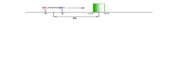
Figure 1: Quantum tunneling of a composite particle through a barrier. The barrier might be visible by only one of the particles, e.g. the neutron within a deuteron does not see a Coulomb barrier due to presence of another nucleus.

There is no need for an external magnetic field if there exists another intrinsic state of the tunneling object that would be able to tunnel with a larger probability. In distinction to the cases of resonant tunneling discussed in the literature the situation is possible when the composite particle energetically cannot be transferred to the state with favorable conditions for tunneling. However, even the virtual admixture of such an intermediate state can increase penetrability. In such a case outside of the barrier the trace of the evanescent state can exist only in the vicinity of the barrier. Similar virtual states emerge with necessity in reflection of a composite particle sato02 as well as in the situation when only one of the constituents interacts with the barrier while the rest of the constituents do not feel it zakhariev64 ; matthews99 ; ahsan07 . This happens for example at the Coulomb barrier for a system that contains neutral and charged constituents (see figure 1).

Next we briefly consider the case when the excited intrinsic state with energy $E^{\prime}>E$ can virtually transfer excitation into translational energy (the system then is still under the barrier). The two-component wave function with the low component describing the new intrinsic state can be written in a form similar to eqs. (1-3), with simple substitutions

$$B^{\prime}e^{-ikx}\Rightarrow B^{\prime}e^{\lambda x},\quad F^{\prime}e^{ik(x-a)}\Rightarrow F^{\prime}e^{-\lambda(x-a)},$$ (12)

where $\lambda=[2m(E^{\prime}-E)]^{1/2}$ gives the decay of the virtual wave function in free space. The wave function inside the barrier still keeps the form (3) with $\kappa^{\prime}$ now describing the imaginary momentum of the virtual state.

The transmission coefficient here is found as

$$T=16k^{2}\,\left[\frac{\kappa(\kappa^{\prime}+\lambda)^{2}e^{-\kappa a}+\kappa^{\prime}(\kappa+\lambda)^{2}e^{-\kappa^{\prime}a}}{\left(2\kappa\kappa^{\prime}+\lambda(\kappa+\kappa^{\prime})\right)^{2}+k^{2}(\kappa+\kappa^{\prime}+2\lambda)^{2}}\right]^{2},$$ (13)

where, analogously to eq. (7) we neglect exponentially small terms. This expression has a simple $\lambda$-independent limit for large excitation energy, $\lambda\gg\kappa,\kappa^{\prime}$, which, under the assumption $\exp(\kappa^{\prime}a)\ll\exp(\kappa a)$, gives

$$T\approx\left[\frac{4k\kappa^{\prime}}{(\kappa+\kappa^{\prime})^{2}+4k^{2}}\right]^{2}\,e^{-2\kappa^{\prime}a}.$$ (14)

This limiting result corresponds to the sudden breakup of the incident wave function by the edge of the barrier that is equivalent to its instantaneous expansion into two components one of which has a strong enhancement of the tunneling probability.

In a more realistic description, the intrinsic wave function of the slow composite particle will change smoothly along its path. We consider a one-dimensional motion of the complex of two particles at positions $(x,y)$ with masses $m_{x}$ and $m_{y}$ coupled by their interaction $V(x-y)$ and slowly moving in an external potential, $U$,

$$H=\frac{p_{x}^{2}}{2m_{x}}+\frac{p_{y}^{2}}{2m_{y}}+V(x-y)+U_{x}(x)+U_{y}(y),$$ (15)

where we allow the external potential $U$ to act differently on the constituents. Introducing the center-of-mass coordinate $R$, relative coordinate $r$, and corresponding masses $M$ and $\mu$ (reduced mass), we come to the stationary Schrödinger equation

$$\left\{-\frac{\hbar^{2}}{2M}\,\frac{\partial^{2}}{\partial R^{2}}-\frac{\hbar^{2}}{2\mu}\,\frac{\partial^{2}}{\partial r^{2}}+V(r)+U_{x}\left(R+\frac{rm_{y}}{M}\right)+U_{y}\left(R-\frac{rm_{y}}{M}\right)-E\right\}\Psi(R,r)=0.$$ (16)

At low energy we can use an adiabatic ansatz

$$\Psi(R,r)=\psi(R)\phi(r;R),$$ (17)

where the internal function $\phi(r;R)$ describing the smooth evolution of relative motion parametrically depends on the slow global variable $R$ and satisfies the instantaneous equation

$$\left\{-\frac{\hbar^{2}}{2\mu}\,\frac{\partial^{2}}{\partial r^{2}}+V(r)+U_{x}\left(R+\frac{rm_{y}}{M}\right)+U_{y}\left(R-\frac{rm_{y}}{M}\right)-\epsilon(R)\right\}\phi(r;R)=0.$$ (18)

A loosely bound state is created by the potential $V(r)$ far away from the barrier. As the motion in the direction of the barrier proceeds and the wings of the relative wave function propagate in the region of the potentials $U$, this wave function is gradually evolving along with its energy eigenvalue $\epsilon(R)$. It was pointed out in FZ05 that the polarizability of the tunneling system by the field of the target may increase the penetration probability.

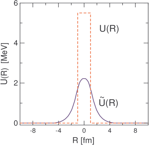
Figure 2: The effective potential $\widetilde{U}(R)$ for the deuteron, as obtained from eq. 23. The dashed line represents the rectangular potential barrier.

Multiplying eq. (16) by $\phi^{\ast}(r;R)$, integrating out the intrinsic variable $r$ and introducing new functions

$$\langle\phi|\phi\rangle=N(R),\quad\langle\phi|\partial\phi/\partial R\rangle=N(R)\alpha(R),\quad\langle\phi|\partial^{2}\phi/\partial R^{2}\rangle=N(R)\beta(R),$$ (19)

the resulting equation for $\psi(R)$ becomes

$$\psi^{{}^{\prime\prime}}+2\alpha(R)\psi^{\prime}+\beta(R)\psi+\frac{2M}{\hbar^{2}}[E-\epsilon(R)]\psi=0,$$ (20)

where primes label the derivatives with respect to $R$. Defining the new function $u(R)$,

$$\psi(R)=u(R)e^{-\int\alpha(R)\,dR},$$ (21)

we reduce the problem to the standard Schrödinger equation,

$$u^{\prime\prime}+\frac{2M}{\hbar^{2}}[E-\tilde{U}(R)]u=0$$ (22)

with the effective potential

$$\tilde{U}{R}=\epsilon(R)-E_{0}+\frac{\hbar^{2}}{2M}\,[\alpha^{2}(R)+\alpha^{\prime}(R)-\beta(R)].$$ (23)

Here the energy scale is chosen in such a way that far from the barrier, $R\rightarrow\infty$, energy $\epsilon(R)$ coincide with the intrinsic binding energy $E_{0}$. Note that the solution of eq. 18 is not normalized. But eq. 17 is, i.e. $\sqrt{N(R)}\psi(R)$ is normalized to one.

The closeness of the continuum level would be dangerous in the form of adiabatic perturbation theory where small denominators can arise. But in the form of a differential equation, as formulated above, we do not throw away non-adiabatic effects. They are important and they make the wave function to evolve. Of course, real dissociation is impossible at low energy because of energy conservation. When the binding energy is small, the particles are still correlated and can get together after the barrier. (Even in the continuum their wave function would not be the product of two independent plane waves, they are still correlated because of the interaction between them.) Our model accounts for these features.

As an application of this approach, we consider the transmission of a composite particle through a rectangular barrier, Fig. 1, a problem discussed for a molecule in the context of condensed matter physics in saito94 ; sato02 . For nuclear applications we assume the “deuteron” model, when the rectangular potential of Fig. 1 acts on one constituent (“proton”) only, $U_{x}=U_{p}$, while its partner, a “neutron”, is not influenced by the barrier, $U_{y}=0$. The intrinsic potential $V(r)$ is also taken as a rectangular well with parameters of depth $V_{0}=11.4$ MeV and width $r_{0}=2$ fm reproducing the deuteron binding energy $E_{0}=-2.225$ MeV. The choice of the barrier parameters, $U_{0}=5.5$ MeV and $a=r_{0}=2$ fm, implies that at $R=0$ the intrinsic well exactly coincides with the barrier and the deuteron is practically unbound. The masses used to produce the results in fig. 2 are $M=2m_{N}$ and $\mu=m_{N}/2$, where $m_{N}=939$ MeV is the free nucleon mass.

The numerically calculated effective potential (23) is shown in Fig. 2 by a solid line. It is obvious that the barrier transmission problem is very different from that for penetration through the original potential $U(R)$, a dashed line. At $R=0$ the deuteron is barely bound with binding energy $\epsilon(0)=0.01$ MeV; the non-adiabatic terms [the brackets in eq. (23)] are very small at $R=0$, so that the height of the effective potential here is only $\tilde{U}(0)\approx 2.21$ MeV, as seen in Fig. 2. For a deeper intrinsic potential $V(r)$, the height $\tilde{U}(0)$ would be closer to the top of the barrier but the smearing effect of weak deuteron binding is significant.

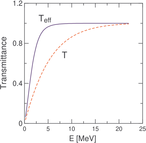
Figure 3: Transmission probability for a deuteron incident on a rectangular barrier (dashed-line) and on an effective potential barrier (solid line). Potential and energy parameters are given in the text.

The Schrödinger equation (22) with the symmetric effective potential $\tilde{U}(R)$ allows, at given energy $E$, for the solutions with definite parity, $u_{\pm}$. The solution of the transmission problem given by the incident wave from the left is their linear combination. We find $u_{+}$ and $u_{-}$ by a numerical procedure starting from the center of the barrier, $R=0$, with

$$u_{+}(0)=1,\quad u_{+}^{\prime}(0)=1,\quad u_{-}(0)=0,\quad u_{-}^{\prime}(0)=1,$$ (24)

and using an arbitrary normalization of these basic solutions. Then we can compute the dimensionless logarithmic derivatives at a remote point $R=R_{0}$, where $\tilde{U}(R_{0})$ is negligible,

$$\Lambda_{\pm}=R_{0}\,\frac{u_{\pm}^{\prime}(R_{0})}{u_{\pm}(R_{0})}.$$ (25)

The logarithmic derivatives at the mirror point $R=-R_{0}$ are $-\Lambda_{\pm}$.

Now we can perform the matching at $R=\pm R_{0}$ for the scattering (transmission) problem with energy $E=\hbar^{2}k^{2}/2M$, where the wave function is

$$u(R)=\left\{\begin{array}[]{cc}e^{ikR}+Be^{-ikR},&-\infty<R\leq-R_{0},\\ C_{+}u_{+}(R)+C_{-}u_{-}(R),&-R_{0}\leq R\leq R_{0},\\ Fe^{ikR},&R_{0}\leq R<\infty.\end{array}\right.$$ (26)

This gives the reflection and transmission amplitudes,

$$B=-\frac{1}{2}\left[\frac{\Lambda_{+}+iq}{\Lambda_{+}-iq}+\frac{\Lambda_{-}+iq}{\Lambda_{-}-iq}\right]e^{-2iq},\quad F=-\frac{1}{2}\left[\frac{\Lambda_{+}+iq}{\Lambda_{+}-iq}-\frac{\Lambda_{-}+iq}{\Lambda_{-}-iq}\right]e^{-2iq},$$ (27)

where $q=kR_{0}$. The transmission probability is given by

$$T=\frac{q^{2}(\Lambda_{+}-\Lambda_{-})^{2}}{(q^{2}+\Lambda_{+}^{2})(q^{2}+\Lambda_{-}^{2})}.$$ (28)

Such a calculation contains a continuous transition to global energy exceeding the height of the effective barrier. However, then one need to take into account the opening of the breakup channels.

The results are shown in Fig. 3 in comparison with the simple tunneling calculation (9) that did not take into account the gradual adjustment of the internal wave function. A considerable enhancement of the tunneling probability is evident.

Of course this is just a simple model that does not pretend to give a realistic quantitative description of tunneling for a composite object. However, we believe that it is worthwhile to point out that there exist quantum-mechanical effects which are not discussed in textbooks and which could be seen even in such a simplified example. Moreover, this simple description allows us to clearly demonstrate physics of the process not overshadowed by cumbersome computations.

We use a trial wave function that corresponds to slow motion of the object as a whole at very low energy when dissociation channels are forbidden. In the framework of this variational approach we solve the problem exactly taking into account non-adiabatic corrections (derivatives of the function describing slow motion) which are usually neglected in a standard Born-Oppenheimer approximation in molecular or solid state physics. This leads to the differential Schroedinger-type equation that is solved exactly (see also aur98 ).

In conclusion, we would like to stress that tunneling of composite objects is an important topic, regrettably not studied in detail. Numerous applications to nuclear, atomic, molecular and condensed matter physics,as well as to astrophysical reactions, make the progress in understanding this problem absolutely necessary.

- (1) A.B. Balantekin and N. Takigawa, Rev. Mod. Phys. 70, 77 (1998).
- (2) N. Saito and Y. Kayanuma, J. Phys.: Condens. Matter 6, 3759 (1994).
- (3) A.V. Arzhannikov, G.Ya. Kezerashvili, Phys. Lett. A156, 514 (1991).
- (4) H. Yuki, J. Kasagi, A.G. Lipson, T. Ohtsuki, T. Baba, T. Noda, B.F. Lyakhov, and N. Asami, Pis’ma Zh. Eksp. Teor. Fiz. 68, 785 (1998) [JETP Lett. 68, 823 (1998)].
- (5) N. Saito and Y. Kayanuma, Phys. Rev. B 51, 5453 (1995).
- (6) T. Sato and Y. Kayanuma, Europhys. Lett. 60, 331 (2002).
- (7) S. Kimura and N. Takigawa, Phys. Rev. C 66, 024603 (2002).
- (8) G.L. Goodvin and M.R. Shegelski, Phys. Rev. A 71, 032719 (2005).
- (9) G.L. Goodvin and M.R. Shegelski, Phys. Rev. A 72, 042713 (2005).
- (10) V.V. Flambaum and V.G. Zelevinsky, J. Phys. G: Nucl. Part. Phys. 31, 355 (2005).
- (11) S. Bacca and H. Feldmeier, Phys. Rev. C 73, 054608 (2006).
- (12) N. Takigawa, Y. Nozawa, K. Hagino, A. Ono, and D. M. Brink, Phys. Rev. C 59, R593 (1999).
- (13) C.A. Bertulani, D.T. de Paula, and V.G. Zelevinsky, Phys. Rev. C 60, 031602 (1999).
- (14) V.V. Flambaum and V.G. Zelevinsky, Phys. Rev. Lett. 83, 3108 (1999).
- (15) B.N. Zakhariev and S.N. Sokolov, Ann. d. Phys. 14, 229 (1964).
- (16) M. Matthews, A. Sakharuk and V. Zelevinsky, BAPS 44, No. 5, p. 37 (1999).
- (17) N. Ahsan and A. Volya, BAPS 52, No. 3, p. 159 (2007).
- (18) A. Bulgac, G. Do Dang and D. Kusnezov, Phys. Rev. E 58, 196 (1998).