The effects of spatially distributed ionisation sources on the temperature structure of H ii regions

Abstract

Spatially resolved studies of star forming regions show that the assumption of spherical geometry is not realistic in most cases, with a major complication posed by the gas being ionised by multiple non-centrally located stars or star clusters. Geometrical effects including the spatial configuration of ionising sources affect the temperature and ionisation structure of these regions. We try to isolate the effects of multiple non-centrally located stars, via the construction of 3D photoionisation models using the 3D Monte Carlo photoionisation code mocassin with very simple gas density distributions, but various spatial configurations for the ionisation sources. Our first aim is to study the resulting temperature structure of the gas and investigate the behaviour of temperature fluctuations within the ionised region. We show that geometry affects the temperature structures in our models differently according to metallicity. For the geometries and stellar populations considered in our study, at intermediate and high metallicities, models with ionising sources distributed in the full volume, whose Strömgren spheres rarely overlap, show smaller temperature fluctuation than their central ionisation counterparts, with fully overlapping concentric Strömgren spheres. The reverse is true at low metallicities. Finally the true temperature fluctuations due to the stellar distribution (as opposed to the large-scale temperature gradients due to other gas properties) are small in all cases and not a significant cause of error in metallicity studies.

Emission line spectra from H ii regions are often used to study the metallicity of star-forming regions, as well as providing a constraint for temperatures and luminosities of the ionising sources. Empirical metallicity diagnostics must often be calibrated with the aid of photoionisation models. However, most studies so far have been carried out by assuming spherical or plane-parallel geometries, with major limitations on allowed gas and dust density distributions and with the spatial distribution of multiple, non-centrally located ionising sources not being accounted for. We compare integrated emission line spectra from our models and quantify any systematic errors caused by the simplifying assumption of a single, central location for all ionising sources. We find that the dependence of the metallicity indicators on the ionisation parameter causes a clear bias, due to the fact that models with a fully distributed configuration of stars always display lower ionisation parameters than their fully concentrated counterparts. The errors found imply that the geometrical distribution of ionisation sources may partly account for the large scatter in metallicities derived using model-calibrated empirical methods.

1 Introduction

The ability to measure accurate chemical abundances in H ii regions in our own and other galaxies is vital for our understanding of their chemical evolution. Emission lines emitted by the nebular gas photoionised by massive stars provide us with powerful metallicity indicators for near and intermediate redshift galaxies. The major complication is posed by the critical task of determining the physical parameters of the nebula, in particular the electron temperature, $T_{\rm e}$. Failure to achieve realistic estimates may lead to gross errors in the final abundance determination. Temperature fluctuations within the nebula may be an important cause of error. Collisionally excited lines (CELs), which are routinely used in abundance studies, are naturally weighted towards hotter regions and may therefore lead to underestimating of the real abundances. Recombination lines (RLs) are less affected by errors in temperature determinations, and should in theory yield more accurate results. One of the outstanding problems in nebular astrophysics is the discrepancy between abundances and electron temperature estimates obtained from CELs or RLs in Planetary Nebulae (PNe) (e.g. Rubin et al. 2002; Wesson, Liu & Barlow 2005; Ercolano et al. 2005; Liu et al. 2006; Peimbert & Peimbert 2006 and references therein), galactic and Magellanic H ii regions (e.g. Peimbert, Peimbert & Ruiz 2000; Peimbert 2003; Tsamis et al. 2003; Esteban et al. 2004; García-Rojas et al. 2005, 2006) and extragalactic H ii regions (e.g. Peimbert & Peimbert 2003; Peimbert, Peimbert & Ruiz 2005). The cause of this discrepancy is still uncertain; temperature fluctuations and chemical inhomogeneities in the gas have both been advocated to explain the discrepancy. Photoionisation models including chemical inhomogeneities have been successful in matching the observed CEL and RL spectra of some PNe (e.g. Ercolano et al. 2003b) and H ii regions (Tsamis & Péquignot 2005). However the discrepancy between the abundances derived from recombination lines (RL) and those derived from CELs has been also been attributed to temperature fluctuations not caused by abundance inhomogeneities (e.g. García-Rojas et al. 2004). The $t^{2}$ parameter (Peimbert, 1967; Peimbert & Costero 1969; Peimbert 1971), introduced in order to quantify such fluctuations, can be derived empirically by the comparison of temperatures obtained from the depth of the Balmer Jump to those obtained from CELs. Although the situation for H ii regions is notoriously less worrying than for PNe, the problem still remains that empirically determined $t^{2}$ values are larger than those indicated by chemically homogeneous photoionisation models, indicating that the causes of the proposed temperature fluctuations are still not understood.

Aside from temperature fluctuations the task of obtaining reliable abundance estimates from CEL spectra of H ii regions is further complicated by the fact that often the complete set of emission lines needed for a direct measurement of the electron temperatures is not available for all sources; the 4363 Å line of $[$O iii$]$ and the 5755 Å line of $[$N ii$]$ are weak and therefore not detected if the spectra do not have good signal-to-noise or if the metallicities are high, implying low electron temperatures. A large effort has been made to provide metallicity and temperature indicators based on various combinations of strong lines (e.g. Pagel et al. 1979; Alloin et al. 1979; Mc Gaugh 1991; Storchi-Bergmann et al. 1994; Vílchez & Esteban 1996; Van Zee et al. 1998; Pilyugin 2001a; Pettini & Pagel 2004; Pérez-Montero & Díaz 2005). Hägele et al. (2006) have recently proposed a new methodology for the production and calibration of empirical relations between the different line temperatures based on observational data alone. However the data sets available are still too limited to provide usable indicators. Currently, calibrations of metallicity indicators and ionic temperature relations are generally not based on observational data alone, but make use of grids of photoionisation models, run for a range of metallicities and ionisation parameters (e.g. McGaugh 1991, Charlot & Longhetti 2001, Kewley & Dopita 2002). Given the vast parameter space generally under investigation, most studies so far have been carried out with spherically symmetric or plane parallel geometries, with major limitations on the allowed density distribution and with the spatial distribution of the ionising sources not being investigated. Nearby H ii regions, however, show complex structures in the distribution of gas and stars, which are often intermixed.

In this paper we carry out a theoretical investigation of the importance of the effects due to the spatial distribution of the ionising sources via the construction of a number of 3D photoionisation models, using the mocassin code (Ercolano et al. 2003a, 2005) for simple gas density distributions and three spatial configurations for the ionisation sources.

Our modelling strategy is described in Section 2. Temperature fluctuations are estimated for our models by computing theoretical $t^{2}$ and $T_{0}$ values (Peimbert, 1967) for each of our models and the results are given and discussed in Section 3. In this Section we also compare integrated emission line spectra from such configurations to search for systematic errors which may be caused by the simplifying assumption of a single, central location for all ionising sources. We also test the robustness of a number of commonly used ionic temperature relations. A summary of our main results is presented in Section 4.

2 Modelling strategy

Table 1: Characterising model parameters. $L_{\rm bol}$ is the total bolometric luminosity of all stars included. $R_{s}$ is the Strömgren radius in the case when all stars are located at the centre of the sphere/shell. The total number of ionising photons and the hydrogen number density are constant for all models and are, respectively, $Q_{\rm H^{0}}$ =  3.80$\cdot$10⁵⁰ sec^-1 and $N_{\rm H}$ = 100 cm^-3. All shell models have an inner radius of 2.8$\cdot$10¹⁹ cm.

Z/Z⊙	$L_{\rm bol}$	$R_{s}$
	$[$E40 erg/sec$]$	$[$E19 cm$]$
		sphere	shell
2.0	3.30	2.65	3.45
1.0	3.00	2.85	3.55
0.4	2.64	3.20	3.75
0.2	2.30	3.45	3.90
0.05	1.98	3.75	4.20

Table 2: Model grid legend. H number density, N_H = 100 $[cm^{-3}]$ for all models. Figures in this paper rely on colour, please refer to on-line version. For black and white copies black is black, blue is dark-gray, red is medium gray and green is light gray.

model	star distrib.	geometry	Z/Z⊙	symbol	model	star distrib.	geometry	Z/Z⊙	symbol
CSp2.0	central	sphere	2.0	small magenta circle	CSh0.4	central	shell	0.4	small red square
HSp2.0	half distrib	sphere	2.0	medium magenta circle	HSh0.4	half distrib	shell	0.4	medium red square
FSp2.0	fully distrib	sphere	2.0	large magenta circle	FSh0.4	fully distrib	shell	0.4	large red square
CSh2.0	central	shell	2.0	small magenta square	CSp0.2	central	sphere	0.2	small green circle
HSh2.0	half distrib	shell	2.0	medium magenta square	HSp0.2	half distrib	sphere	0.2	medium green circle
FSh2.0	fully distrib	shell	2.0	large magenta square	FSp0.2	fully distrib	sphere	0.2	large green circle
CSp1.0	central	sphere	1.0	small black circle	CSh0.2	central	shell	0.2	small green square
HSp1.0	half distrib	sphere	1.0	medium black circle	HSh0.2	half distrib	shell	0.2	medium green square
FSp1.0	fully distrib	sphere	1.0	large black circle	FSh0.2	fully distrib	shell	0.2	large green square
CSh1.0	central	shell	1.0	small black square	CSp0.05	central	sphere	0.05	small green circle
HSh1.0	half distrib	shell	1.0	medium black square	HSp0.05	half distrib	sphere	0.05	medium green circle
FSh1.0	fully distrib	shell	1.0	large black square	FSp0.05	fully distrib	sphere	0.05	large green circle
CSp0.4	central	sphere	0.4	small red circle	CSh0.05	central	shell	0.05	small green square
HSp0.4	half distrib	sphere	0.4	medium red circle	HSh0.05	half distrib	shell	0.05	medium green square
FSp0.4	fully distrib	sphere	0.4	large red circle	FSh0.05	fully distrib	shell	0.05	large green square

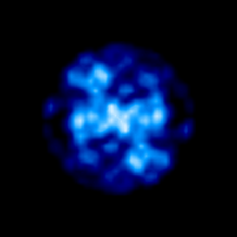
Figure 1: The left panel shows a 3D representation of the Strömgren sphere distribution for case F, plotted as the iso-surfaces where the ionisation fraction of hydrogen is 0.95. The adjacent right panel shows an average projection map of the ionic abundance of H⁺.

The aim of the current investigation is to uncover possible systematic differences on the temperature structure and emission line spectra of nebulae ionised by a centrally concentrated set of stars or clusters versus those ionised by the same set of sources which are randomly distributed within the half or full volume, whose respective Strömgren spheres do or do not overlap. In particular we want to test which of the stellar configurations considered produces the largest temperature fluctuations and of what magnitude. At this stage we do not attempt to assess the absolute strengths and weaknesses of one metallicity indicator or ionic temperature relation over others, a task that may only be carried out by a systematic investigation of the large parameter space. In an attempt to isolate the effects of the stellar distribution from those due to the gas density distribution, we consider two extremely simple geometries - a homogeneous spherical volume and a homogeneous spherical shell, both of constant hydrogen number density, $N_{\rm H}$ = 100 cm^-3. The shell models have inner radii of 2.8$\cdot$10¹⁹ cm and Strömgren radii (corresponding to the case when all stars are located at the centre) as listed in Table 1. The total number of ionising photons is constant for all models and is $Q_{\rm H^{0}}$ = 3.80$\cdot$10⁵⁰ sec^-1.

For each density distribution we are interested in a comparison between the centrally concentrated and the half and fully distributed source cases. In the remainder of this paper we will refer to models ionised by a central concentration of stars as models C, those ionised by the same set of stars distributed in the half and full volumes will be referred to as models H and F, respectively. Case C is equivalent to models ionised by a single central source with a total bolometric luminosity equal to the sum of the bolometric luminosities of the individual sources (as given in Table 1) and a spectral shape given by the superposition of the spectra of all sources. These models could also be performed using a 1D code, with a spherically symmetric gas density distribution. Similarly a 1D code could also be employed for case F models where the Strömgren spheres do not generally overlap; the left panel of Figure 1 shows a 3D representation of the Strömgren sphere distribution for case F, plotted as iso-surfaces where the ionisation fraction of hydrogen is 0.95. The adjacent panel shows a projected map of the ionic abundance of H⁺. In the intermediate case, case H, the Strömgren spheres of most H ii regions partially overlap; the determination of the radiation field in the overlap region is not possible without the application of a 3D code. As we are interested in a comparison of the three cases (C, H and F), self-consistency is crucial and for this reason we have run all models with the same 3D code, mocassin.

Our models include five metallicities ($Z/Z_{\odot}$ = 0.05, 0.2, 0.4, 1.0, 2.0). The ”solar” abundance set uses the values from Grevesse & Sauval (1998) with the exception of C, N, O abundances which are taken from Allende Prieto et al 2002, Holweger 2001 and Allende Prieto et al 2001, respectively. These were scaled to lower and higher metallicities considering the empirical abundance trends observed in H ii regions by Izotov et al. (2006). In order to maximise the effects of spatially distributed sources whose Strömgren spheres may overlap (completely or partially), or be totally independent, we consider the limiting case of an ionising set composed of two stellar populations, a 37 M_⊙ and a 56 M_⊙ population, with half of the total ionising photon output [s^-1] being emitted by each population. These two stellar masses were chosen as they have very different $Q_{\rm He^{0}}$/$Q_{\rm H^{0}}$ ratios, where $Q_{\rm H^{0}}$ is the total output [s^-1] of H-ionising photons (energy $>$ 1 ryd) and $Q_{\rm He^{0}}$ is the total output [s^-1] of He-ionising photons (energy $>$ 1.8 ryd), and are likely to produce the largest effects on the temperature structure and sharpness of the ionisation front. The ionising spectra for single-mass stars were computed with the starburst99 spectral synthesis code Leitherer et al. (1999) with the up-to-date non-LTE stellar atmospheres implemented by Smith, Norris & Crowther (2002), using single isochrones for the appropriate stellar masses. The models were calculated at metallicities consistent with the nebular gas and were obtained for an instantaneous burst, at an age of 1 Myr. At solar metallicities for the 37 M_⊙ stars, the stellar atmosphere models emit 32.3% of luminosity in the H-ionising continuum and 7.7% in the He-ionising continuum, while for the 56 M_⊙ stars these percentages are 47.9% and 13.7%, respectively. The exact percentages vary with stellar metallicity, nevertheless the values above are given as a guide to appreciate the different spectral hardness of the two populations.

Some other defining parameters of our models, together with their nomenclature and associated symbols are given in Table 2.

2.1 The 3D photoionisation code: mocassin

The 3D photoionisation code mocassin (Ercolano et al. 2003a, 2005) uses a Monte Carlo approach to the radiation transport problem and it is therefore completely independent of geometry and density distribution. Both the stellar and diffuse components of the radiation field are treated self-consistently, without the need of approximations. Multiple ionisation sources can be located at arbitrary positions in the simulation grid with the only limit being imposed by computing resources. The atomic data used is frequently updated and include sets of energy levels, collision strengths and transition probabilities from Version 5 of the Chianti database (Landi et al., 2005) and the improved H i, He i and He ii free-bound continuous emission data recently published by Ercolano & Storey (2006). A public version of the fortran 90 code, which is fully parallelised using the Message Passing Interface (MPI) libraries, can be obtained from B. Ercolano. Version 2.02.38 was used for the models presented in this work. We simulate one quadrant of each model, using the technique described and tested by Ercolano et al. (2003b), whereby the positive x-y, y-z and x-z planes intersecting the z-, x- and y- axes respectively at zero, act as mirrors, reflecting the incoming photons back into the simulated cube. The full volume is finally described by 10⁶ cells for the shell models and by 125000 cells for the spherical models ionised by 240 sources. The number of energy packets used varies during the course of our simulations, but typically 1-10 million packets are sufficient for our grids to reach convergence within 10-20 iterations. We experimented with higher resolution grids and a larger number of energy packets and found our results to be virtually unaffected.

2.2 Validation of our models

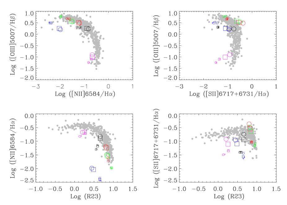
Figure 2: H ii region excitation sequence in terms of $[$N ii$]$/H$\alpha$ and $[$S ii$]$/H$\alpha$ vs.$[$O iii$]$/H$\beta$ and R23. The grey points represent giant H ii regions in galaxies taken from Garnett & Kennicutt (1994), Garnett et al. (1997), van Zee et al. (1998), Bresolin et al. (1999, 2004, 2005), and Kennicutt et al. (2003), spanning metallicities from 12 + log(O/H) $\sim$ 8 to $\sim$ 8.8., and metal-poor emission line galaxies from Izotov et al. (2006), which extend to 12 + log(O/H) $\sim$ 7.2. The symbols and colors correspond to our models as defined in Table 2. Please refer to the on-line version of this paper for colour figures.

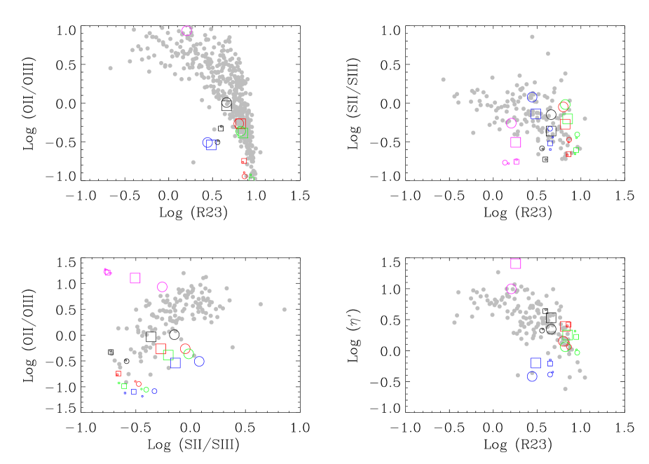
Figure 3: H ii region ionisation sequence parametrised in terms of oxygen and sulphur. The grey dots indicate the position of giant H ii regions in spiral galaxies taken from Garnett & Kennicutt (1994), Garnett et al. (1997), van Zee et al. (1998), Bresolin et al. (1999, 2004, 2005), Kennicutt et al. (2003), spanning metallicities from 12 + log(O/H) $\sim$ 8 to $\sim$ 8.8. The top right panel also includes a few points from metal-poor emission line galaxies from Izotov et al. (2006), which extend to 12 + log(O/H) $\sim$ 7.2; it was not possible to use this data for the other three panels, due to the lack of simultaneous detection of all the lines needed. The symbols and colors correspond to our models as defined in Table 2. Please refer to the on-line version of this paper for colour figures.

As stated above, the aim of this paper is not to provide new calibrations to abundance diagnostic ratios nor to assess their absolute accuracy. It is therefore not in our intention to create models that fit any particular observations. While trying to maximise the effects of a complex ionising field distribution, it is however still necessary to ensure that the ionisation and temperature structures and, hence, emission line ratios we obtain from our models are in the range of those observed in nature. In Figure 2 we plot our results in a number of line ratio diagrams, including those following Veilleux & Osterbrock (1987) and Osterbrock, Tran & Veilleux (1992), that show the variation in $[$N ii$]$ and $[$S ii$]$ excitation parametrised in terms of $[$O iii$]/H\beta$ (top panels) and those following Mc Call, Rybski & Shields (1985) showing the variation in terms of R23. Similarly, in Figure 3 we plot the H ii region ionisation sequence parametrised in terms of oxygen and sulphur line ratios . The grey dots represent giant H ii regions in spiral galaxies, taken from Garnett & Kennicutt (1994), Garnett et al. (1997), van Zee et al. (1998), Bresolin et al. (1999, 2004, 2005), and Kennicutt et al. (2003), spanning metallicities from 12 + log(O/H) $\sim$ 8 to $\sim$ 8.8. Figure 2 and the top right panel of figure 3 also include a few points from metal-poor emission line galaxies from Izotov et al. (2006), which extend to 12 + log(O/H) $\sim$ 7.2; it was not possible to use this data for the other three panels of figure 3, due to the lack of simultaneous detection of all the oxygen and sulphur lines needed. In general, our models fall within or near the locus of observed H ii regions, with the exception of our lowest metallicity ($Z/Z_{\odot}~{}=~{}0.05$) and highest metallicity ($Z/Z_{\odot}~{}=~{}2$) models, which is not surprising given that the observational sets available did not include many data points at such extreme values of $Z$; furthermore we did not attempt any systematic variation of the ionisation parameter with $Z$, while observations of giant H ii regions argue that the ionisation parameter decreases as $Z$ increases (see e.g. Mc Gaugh 1994). However this does not affect the achievement of our aims.

3 Results

The temperature structure and emission line spectra obtained by our models are analysed here in detail. Temperature fluctuations, which may introduce errors in the empirical calculations of abundances, are examined. The robustness of commonly used abundance diagnostics and ionic temperature relations are also tested against possible errors introduced by geometrical effects.

3.1 Temperature structure

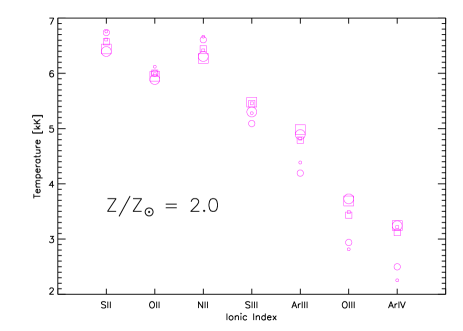
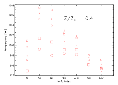
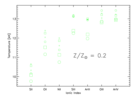
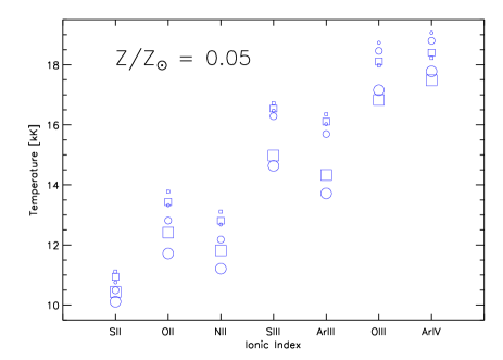
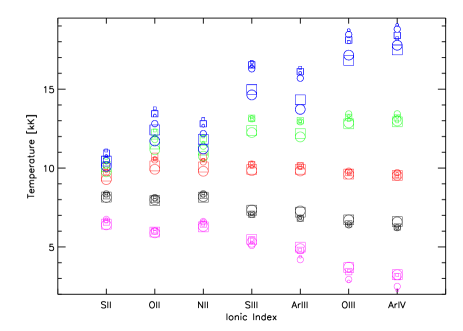
Figure 4: Volume integrated electron temperatures weighted by ionic species. Top left: results for all models with $Z/Z_{\odot}$ = 2 (magenta); top right: results for all models at $Z/Z_{\odot}$ = 1 (black); middle left: results for all models at $Z/Z_{\odot}$ = 0.4 (red); middle right: results for all models at $Z/Z_{\odot}$ = 0.2 (green); bottom left: results for all models at $Z/Z_{\odot}$ = 0.05 (blue); bottom right: Results for all models at all metallicities. A legend for the symbols is given in Table 2. Please refer to the on-line version of this paper for colour figures.

Table 3: Mean temperatures and temperature fluctuations quantified in terms of $T_{0}$(H⁺), $t^{2}$(H⁺), $T_{0}$(O⁺), $t^{2}$(O⁺),$T_{0}$(O²⁺) and $t^{2}$(O²⁺) (Peimbert, 1967)

model	$T_{0}(H^{+})$	$t^{2}(H^{+})$	$T_{0}(O^{+})$	$t^{2}(O^{+})$	$T_{0}(O^{+2})$	$t^{2}(O^{+2})$
CSphH0.05	18240	0.0178	13350	0.041	18500	0.007
HSphH0.05	17690	0.0228	12830	0.046	18500	0.007
FSphH0.05	14850	0.0511	11720	0.035	17180	0.009
		$\pm$ 0.0006		$\pm$ 0.003		$\pm$ 0.004
CSphH0.2	13140	0.0034	12060	0.0145	13430	0.0010
HSphH0.2	13230	0.0036	11810	0.0156	13430	0.0005
FSphH0.2	12100	0.0112	11160	0.0141	12860	0.0010
		$\pm$ 0.0001		$\pm$ 0.0004		$\pm$ 0.0001
CSphH0.4	9850	0.0063	10620	0.0069	9790	0.0053
HSphH0.4	9860	0.0038	10500	0.0060	9790	0.0029
FSphH0.4	9710	0.0036	9910	0.0047	9600	0.0024
		$\pm$ 0.0005		$\pm$ 0.0007		$\pm$ 0.0003
CSphH1.0	6690	0.024	8130	0.020	6380	0.012
HSphH1.0	6670	0.021	8110	0.020	6380	0.009
FSphH1.0	7320	0.018	7990	0.012	6710	0.009
		$\pm$ 0.006		$\pm$ 0.002		$\pm$ 0.001
CSphH2.0	5000	0.156	6110	0.043	2910	0.130
HSphH2.0	4880	0.152	5980	0.050	2919	0.096
FSphH2.0	5360	0.075	5890	0.036	3700	0.084
		$\pm$ 0.005		$\pm$ 0.003		$\pm$ 0.003
CShhH0.05	17510	0.0129	13770	0.0437	18110	0.0041
HShhH0.05	17520	0.0166	13440	0.0438	18110	0.0057
FShhH0.05	15200	0.0369	12410	0.0348	16840	0.0098
		$\pm$ 0.0002		$\pm$ 0.0002		$\pm$ 0.0001
CShhH0.2	12940	0.0033	12390	0.0113	13210	0.0017
HShhH0.2	13080	0.0029	12250	0.0124	13210	0.0010
FShhH0.2	12280	0.0082	11520	0.0121	12810	0.0015
		$\pm$ 0.0002		$\pm$ 0.0002		$\pm$ 0.0007
CShhH0.4	9780	0.0091	10570	0.0089	9710	0.0078
HShhH0.4	9880	0.0084	10740	0.0081	9710	0.0068
FShhH0.4	9810	0.0060	10130	0.0064	9620	0.0046
		$\pm$ 0.0003		$\pm$ 0.0003		$\pm$ 0.0001
CShhH1.0	6880	0.030	7980	0.026	6460	0.017
HShhH1.0	6850	0.029	8010	0.026	6460	0.016
FShhH1.0	7280	0.021	7940	0.017	6720	0.012
		$\pm$ 0.001		$\pm$ 0.001		$\pm$ 0.001
CShhH2.0	5450	0.086	5980	0.045	3420	0.09
HShhH2.0	5430	0.090	6000	0.045	3420	0.09
FShhH2.0	5490	0.070	5950	0.037	3690	0.08
		$\pm$ 0.006		$\pm$ 0.006		$\pm$ 0.01

The volume integrated electron temperatures weighted by a number of commonly observed ionic species are plotted in Figure 4 for metallicities of $Z/Z_{\odot}$ = 0.05, 0.2, 0.4, 1 and 2. The values were obtained according to

$$T_{e}({\rm X^{+i}})=\frac{\int N_{\rm e}N({\rm X^{+i}})T_{\rm e}\,dV}{\int N_{\rm e}N({\rm X^{+i}})\,dV}$$ (1)

The models are represented by circles and squares of various colours and sizes as described in Table 2.

At a first glance some trends are apparent. At solar and high metallicities (i.e. $Z/Z_{\odot}~{}\geq~{}$1) the electron temperatures in ’high’ ionic species zones (e.g. O iii, S iii, Ar iii and N iii) are higher for models in cases H and F. The opposite is true for electron temperatures in ’low’ ionic species zones, such as O ii and N ii. This implies a shallower temperature gradient for case F and H when compared to case C, since at these metallicities the highest nebular temperatures are reached in the low ionisation zones which are not affected by the very efficient cooling provided by the IR fine-structure lines of $[$O iii$]$ as in the high ionisation zones, where, in fact, the lowest temperatures are reached. The $Z/Z_{\odot}$ = 0.05 and 0.2 models do not follow the same trend; here there is a monotonic shift of temperatures, whereby C models are hotter than the H and F models, regardless of ionic species zone. At intermediate metallicities ($Z/Z_{\odot}$ = 0.4) we are in a transition case from the two separate behaviours described above. At low metallicities, the cooling is dominated by collisional excitation of H Ly$\alpha$, which increases as one gets closer to the ionisation front, where the proportion of residual neutral hydrogen increases. This results in a outward decreasing temperature, contrary to the high metallicity cases.

Differences in the temperature structure of cases F and C can be understood as follows: at each point in the nebula the electron temperature is primarily determined by the average energy of the photons absorbed by H and He and by the cooling efficiency of the ions. The latter is naturally less important at lower metallicities. However, for the intermediate to high metallicity cases, it is differences in the distribution of the cooling ions rather than differences in the heating rates which explains the difference in temperature structure between case C and case H for higher and intermediate metallicities.

3.2 Temperature Fluctuations

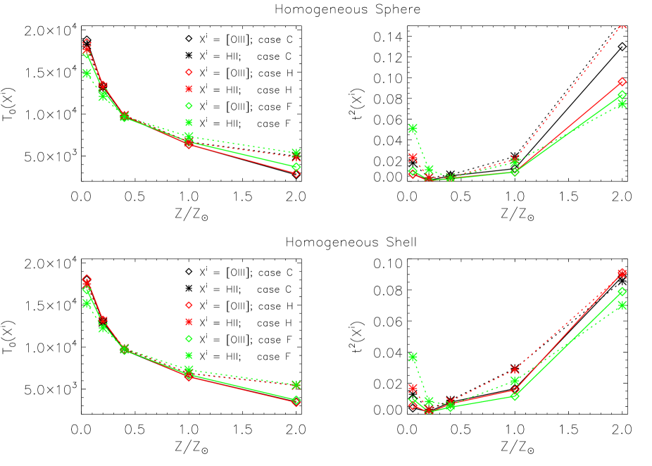
Figure 5: Mean ionic temperatures and temperature fluctuations as a function of gas metallicity for the homogeneous sphere and shell models. $t^{2}(O^{2+})$ and $t^{2}(H~{}^{+})$ are represented by solid and dashed lines, respectively. The lines are colour coded such that black, red and green are for cases C, H and F, respectively. Please refer to the on-line version of this paper for colour figures.

We have calculated for the main ionic species in our models the formal values of the mean ionic temperatures, T₀, and of the temperature fluctuations, $t^{2}$, according to the formalism of Peimbert (1967). Note that in the case of concentric sources, $t^{2}$ measures changes in radial gradients of the temperature rather than “temperature fluctuations” while in the cases of distributed sources it really represent a temperature fluctuation. For brevity we only list the values for H⁺, O⁺ and O²⁺ in Table 3. The errors quoted in the table are representative of the accuracy achieved by our models. They contain contributions from the variance intrinsic to our Monte Carlo approach and the error introduced by using a finite grid to describe the ionised region. The errors were estimated by considering that for a fully spherically symmetric case, such as one with homogeneous gas density distribution and a central location for all ionising sources, the $t^{2}$ in an infinitely narrow spherical shell centred on the source of the ionising photons should be zero. We note that our errors increase with increasing metallicities, this is due to the larger temperature gradients occurring at higher metallicities causing the error contribution due to the finite grid description to increase. Clearly all errors could be reduced by increasing the number of energy packets and grid cells used in the simulations. However we note that our errors are always at least one order of magnitude smaller than the $t^{2}$ values and therefore do not affect our conclusions. Given the large number of 3D models run for this work (which vastly exceeds those finally presented here), we feel that a good balance between accuracy and computational expense was achieved.

The value of $t^{2}$(O⁺) is very hard to derive empirically. We know however of three H ii regions where this measurement has been made: the Orion nebula (Esteban et al. 2004), M20 (García-Rojas et al., 2006) and M8 (García-Rojas et al. 2007). In those cases where $t^{2}$(O⁺) cannot be derived empirically, it is generally assumed that $t^{2}$(O⁺) = $t^{2}$(O²⁺); it is clear from the values listed in our table that this assumption is very often not verified and care should be taken to account for this in the error estimation from such studies. For our $Z/Z_{\odot}$ = 2 models, $t^{2}$(O²⁺) is always a factor of 2 or more higher than $t^{2}$(O⁺), while for lower metallicities $t^{2}$(O²⁺) becomes lower than $t^{2}$(O⁺) sometimes by large factors (up to approximately 10). Finally, we note that the formal $t^{2}$ values may diverge from the empirical ones (e.g. Kingdon & Ferland, 1995; Zhang, Ercolano & Liu, 2007), that are generally based on the comparison of the electron temperature derived from the depth of the Balmer jump and the $[$O iii$]$ temperature, the values listed in Table 3 are, nevertheless, sufficient to identify the effects of the stellar distribution on temperature fluctuations in the nebular gas.

In Figure 5 we plot the $t^{2}$ values for H⁺ and O²⁺ (dashed and solid lines, respectively) against metallicity for the spherical and shell models. Cases C, H and F are represented by black, red and green lines and symbols respectively. Unsurprisingly, the temperature fluctuations, which in this case are a direct consequence of large-scale temperature gradients, are larger for the high metallicity models. A full discussion of this effect and of the causes of the large scale temperature fluctuations in metal rich nebulae is given by Stasińska (1980) and Kingdon & Ferland (1995). What had not been noticed before, however, is that at very low metallicities, the $t^{2}$ values for H⁺ and O⁺ rise again; this is due to the large temperature gradient already shown in Figure 4. However, $t^{2}$(O²⁺) remains tiny, so that the overall effect on abundance determinations is expected to be small.

With regards to a comparison of the $t^{2}$ values obtained with the three different spatial distributions of sources (cases C, H and F), we first of all notice that for intermediate to high metallicities ($Z/Z_{\odot}~{}\geq~{}0.4$), case F models show a more isothermal gas (smaller $t^{2}$) than case H or C models. This is due to the fact that the contributions to the $t^{2}$ due to the true temperature fluctuations created by the two different stellar populations in case F (and in a smaller degree in case H) are completely washed out by the large-scale temperature gradients caused by the metals’ cooling. This effect vastly dominates at these metallicities, resulting in larger values of $t^{2}$ being obtained by case C models, which, as discussed in the previous section (see Figure 4), have steeper temperature gradients than their cases H and F counterparts.

The above is further confirmed by the fact for very low metallicities (Z/Z${}_{\odot}~{}\leq~{}0.2$), case F models (green lines) show larger fluctuations than case C and H models. This is because at these low metallicities, case C, H and F all show similar large-scale temperature gradients (see Figure 4); the values of $t^{2}$ are thus larger for case F models where true temperature fluctuations are at play. However, once again we point out that no large effects are expected on abundance determinations due to the fact that $t^{2}$(O²⁺) is small in all cases.

3.3 Ionic temperature relations

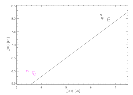
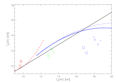
Figure 6: T_e(O ii) versus T_e(O iii) for Z/Z_⊙ =1.0 and 2.0 left and Z/Z_⊙ =0.05, 0.2 and 0.4 right models for cases C, H and F. The straight black solid line is the scaling law of Garnett (1992) and the blue dotted and red dashed curves are the relations given in Eqn 14 of Izotov et al. (2006) for 12 + log(O/H) = 8.2 (red), 7.6 (blue dotted, thick) and 7.2 (blue dotted, thin). The symbols representing our models are described in Table 2. Please refer to the on-line version of this paper for colour figures.

Table 4: Oxygen abundances derived applying various metallicity indicators to the integrated emission line spectra calculated for our models (See text for calibrations used). All abundances are given in logarithmic scale, 12 + log(O/H). The input values of 12 + log(O/H) (i.e. ’the right answer’) are 8.99 (Z/Z_⊙ = 2), 8.69 (Z/Z_⊙ = 1), 8.29 (Z/Z_⊙ = 0.4), 7.99 (Z/Z_⊙ = 0.2) and 7.39 (Z/Z_⊙ = 0.05). $\mid\Delta\mid$, the largest difference between the abundance derived from C, H and F cases are given for each model trio. The value averaged over all models, $\mid<\Delta>\mid$, is given in the last row of the table.

model	O23	O3N2	N2	S23	S3O3	Ar3O3	model	R23	O3N2	N2	S23	S3O3	Ar3O3
CSp2.0	8.67	8.78	8.44	7.92	8.77	8.83	CSh2.0	8.62	8.77	8.50	8.09	8.75	8.82
HSp2.0	8.69	8.78	8.43	7.87	8.76	8.81	HSh2.0	8.62	8.77	8.50	8.08	8.75	8.82
FSp2.0	8.67	8.73	8.52	8.17	8.67	8.78	FSh2.0	8.63	8.76	8.52	8.16	8.72	8.81
$\mid\Delta\mid$	0.02	0.05	0.09	0.30	0.10	0.05	$\mid\Delta\mid$	0.01	0.01	0.02	0.08	0.03	0.01
CSp1.0	8.74	8.27	8.17	7.76	8.04	8.48	CSh1.0	8.66	8.30	8.24	7.94	8.16	8.55
HSp1.0	8.75	8.27	8.16	7.73	8.02	8.46	HSh1.0	8.67	8.30	8.23	7.92	8.14	8.54
FSp1.0	8.49	8.40	8.43	8.34	8.24	8.62	FSh1.0	8.51	8.38	8.39	8.23	8.24	8.61
$\mid\Delta\mid$	0.26	0.13	0.27	0.61	0.22	0.16	$\mid\Delta\mid$	0.16	0.08	0.16	0.31	0.10	0.07
CSp0.4	8.52	8.07	7.87	7.93	8.28	7.96	CSh0.4	8.52	8.09	7.97	8.49	8.10	7.77
HSp0.4	8.52	8.06	7.85	7.92	8.22	7.91	HSh0.4	8.50	8.10	7.98	8.45	8.08	7.73
FSp0.4	8.43	8.24	8.15	8.22	9.02	8.25	FSh0.4	8.41	8.23	8.19	8.92	8.27	8.12
$\mid\Delta\mid$	0.09	0.18	0.30	0.30	0.80	0.34	$\mid\Delta\mid$	0.11	0.14	0.22	0.47	0.19	0.39
CSp0.2	7.86	7.97	7.77	7.99	7.67	7.67	CSh0.2	7.84	7.99	7.79	8.18	7.87	7.92
HSp0.2	7.87	7.97	7.77	8.01	7.66	7.66	HSh0.2	7.86	7.97	7.77	8.10	7.79	7.82
FSp0.2	7.68	8.15	8.05	8.68	8.10	8.26	FSh0.2	7.72	8.13	8.02	8.61	8.11	8.26
$\mid\Delta\mid$	0.19	0.18	0.28	0.69	0.44	0.60	$\mid\Delta\mid$	0.14	0.16	0.25	0.51	0.32	0.44
CSp0.05	7.48	7.92	7.51	7.29	7.39	6.30	CSh0.05	7.44	7.93	7.51	7.38	7.58	6.67
HSp0.05	7.44	7.95	7.56	7.37	7.49	6.51	HSh0.05	7.44	7.94	7.53	7.38	7.57	6.63
FSp0.05	7.15	8.12	7.77	7.73	7.91	7.48	FSh0.05	7.21	8.09	7.74	7.69	7.93	7.49
$\mid\Delta\mid$	0.33	0.20	0.26	0.44	0.52	1.18	$\mid\Delta\mid$	0.23	0.16	0.23	0.31	0.36	0.86
$<\mid\Delta\mid>$	0.18	0.15	0.24	0.47	0.41	0.47	$<\mid\Delta\mid>$	0.12	0.11	0.18	0.32	0.23	0.45

We have shown that the temperature structure of models with centrally concentrated ionising sources, case C, may vary compared to those of similar models where the sources are distributed within the half volume (case H), which have partially overlapping Strömgren spheres, and to those with sources distributed within the full volume (case F), which have fully independent Strömgren spheres. Case C to case F variations in the temperature structure of the models may have implications for a number of ionic temperature relations. These scaling laws are often employed in abundance studies when observational data for a given ionic zone is missing. Some of the most popular relations we found in the literature include T_e(S iii) vs T_e(Ar iii), T_e(O iii) vs T_e(Ar iii), T_e(O ii) vs T_e(N ii). These ratios are expected to be around unity and we found them to be very little affected by the shifts in temperatures due to the spatial distribution of stars. This is not surprising, given that the ionic species involved are both ’high’ (O iii, S iii, Ar iii and N iii) or ’low’ (O ii and N ii), and therefore while the absolute temperature values in each case may shift to higher or lower values, the resulting ratios remain virtually unaffected.

Scaling laws have also been derived for T_e(O iii) vs T_e(S iii) and T_e(O iii) vs T_e(O ii), by Garnett (1992), based on his own grids of photoionisation models and those by Stasińska (1982). More recently, Izotov et al. (2006) produced somewhat different relations between T_e(O ii) and T_e(O iii), and between T_e(S iii) and T_e(O ii) (their Eqs. 14 and 15, valid only for metal poor cases to 12 + log(O/H) $\sim$ 8.2), based on a set of up-to-date (but still spherically symmetric) photoionisation models that reproduce the observed trends of metal-poor galaxies. They found that the observed values of T_e(O ii), T_e(O iii) and T_e(S iii) in a large sample of H ii galaxies reproduce the theoretical relations, but with a large scatter (not only attributable to observational errors in the case of T_e(O ii), T_e(O iii), see their Figures 4a and b).

Figure 6 shows the behaviour of our Z/Z_⊙ =1.0 and 2.0 (left panel, black and magenta symbols respectively) and Z/Z_⊙ =0.05, 0.2 and 0.4 (right panel, blue, green and red symbols, respectively) metallicity models for cases C, H and F with regards to the T_e(O ii) versus T_e(O iii) scaling laws of Garnett (1992, black solid line in both panels) and Izotov et al. (2006, coloured curves in the right panels). The symbols are as described in Table 2. Our lowest metallicity bin Z/Z_⊙ = 0.05 (corresponding to 12 + log(O/H)= 7.39) falls in between Izotov’s 12 + log(O/H)= 7.2 and 7.6 metallicity bins. Their T(O iii) versus T(O ii) relations given in their Eqns 14 are therefore plotted in blue in the right panel of our Figure 6, with the thinner and thicker curves indicating the 7.2 and 7.6 metallicity bin, respectively. Our Z/Z_⊙ = 0.4 metallicity bin (red symbols) corresponds to 12 + log(O/H)= 8.29, slightly above Izotov’s 12 + log(O/H) = 8.2 bin which, nevertheless is represented by the red line in Figure 6.

A ’mixed’ relation such as T_e(O iii) vs T_e(O ii) is much more affected by the fact that low and high ionic temperatures shift in opposite directions for intermediate (red points; Z/Z_⊙ = 0.4) and high metallicities (magenta and black points; Z/Z_⊙ = 2 and 1). This will contribute to the scatter noticed observationally for this relation. For example, Kennicutt, Bresolin & Garnett (2003) presented a study of those H ii regions in M 101 for which direct measurements of the nebular auroral lines could be obtained. They found the T_e(O iii) vs T_e(S iii) relation to be matched closely by their observations, whereas the T_e(O iii) and T_e(O ii) temperatures turned out to be rather uncorrelated. It is also worth noting at this point tht another factor that could contribute to the scatter in the T_e(O iii) vs T_e(O ii) relation is the dependency of T_e(O ii) on the electron density (Pérez-Montero & Díaz 2003). The scatter found by our models is for a given electron density, and therefore it may be even larger for a different sample covering a wider range of densities. The ionising flux distribution is certainly a factor that contributes to weakening the correlation, however, as pointed out by Stasińska (2005), at high metallicities, the temperature derived from the $[$O ii$]$ line ratio may by strongly in error due to the contribution of recombination from O⁺⁺.

3.4 Abundance diagnostics

We have assessed that the geometrical distribution of stars within an H ii region plays a role in the temperature structure of the gas, the magnitude of these effects will clearly be dependent on the total mass of the stars and the concentration level. It is important now to verify the robustness of commonly used metallicity indicator against these temperature shifts. In particular we are interested in identifying systematic trends with stellar distribution rather than absolute errors. Table 4 lists the empirical oxygen abundances obtained using 6 different indicators. We used the following calibrations for the 6 indicators: (1) O₂₃ – Pilyugin (2000, 2001b), (2) O₃N₂ – Stasińska (2006), (3) N₂ – Pettini & Pagel (2004), (4) S₂₃ – Pérez-Montero & Díaz (2005), (5) S₃O₃ – Stasińska (2006), (6) Ar₃O₃ – Stasińska (2006). It is worth reiterating at this point that metallicity indicators should, and generally are, only used for statistical studies as the error on a single region may be very large; the models presented in this work do not attempt to cover the full parameter space occupied by H ii regions and therefore do not aim at identifying the most accurate indicator in absolute terms. Here we are mainly interested in studying a possible systematic error in the derived abundances introduced by the 3D stellar distribution. For this reason for each trio of models (C, H and F for a given density distribution and metallicity) we compute $\Delta$, the largest difference between the oxygen abundance in log units derived from cases C, H and F.

The results are summarised in Table 4, where the mean values $<\Delta>$ are also listed. For all metallicity indicators apart from O₂₃, there is a clear trend for higher metallicity being derived from models ionised by fully distributed sources, case F, than from case C and H models. The reverse is true for O₂₃, where metallicities derived from case F models are smaller than those derived from case C and H models. The $\Delta$ values at a given metallicity vary from one indicator to the next, however they are rarely below $\sim$0.1 dex (only for the highest metallicity case), with more representative values around 0.3 dex for the spherical case, but often larger than 0.4 (and larger than 1.1 dex in one case). These deviations are slightly smaller for the shell density distributions; this is obvious as even for F cases most of the ionising radiation in these models will be emitted from the central cavity, reducing the differences between C and F cases. We note that in some cases the values given by the case H models are lower than those given by the respective case C models (rather than being equal or in the middle between C and F). We have analysed these deviations statistically and can confirm that the small differences are simply due to the variance of our Monte Carlo models and do not bear any physical significance.

The reason for the systematic effect we see in the empirical abundance determinations can be understood by re-examining Figure 3, where the ionisation sequence of our model is parametrised in terms of oxygen and sulphur emission lines. The C (small symbols), H (medium symbols) and F (large symbols) form a sequence, with the case F models generally showing a lower ionisation parameter than case C and H models. The differences in the abundances derived from case C to F with the various indicators clearly reflect the different dependence of each indicator on the ionisation parameter. This can be simply shown for an idealised system. The ionisation parameter of a pure-hydrogen spherical volume of gas with number density $N_{H}$ ionised by a source emitting $Q_{H^{0}}$ hydrogen-ionising photons per second is defined as $U$ = $Q_{H^{0}}$/(4$\pi N_{H}R_{s}^{2}$), where $R_{s}$ is the Strömgren radius. In such a system, from the ionisation balance equation (e.g. Osterbrock, 1989, eqn 2.19) $R_{s}$ is directly proportional to $Q_{H^{0}}^{1/3}$ and to $N_{H}^{-2/3}$, neglecting the temperature dependence of the hydrogen recombination coefficient. For simplicity we compare the ionisation parameter of the system above, $U^{C}$, ionised by only one source, to that of a similar system (F) ionised by $N_{s}$ identical sources each emitting $Q_{H^{0}}$/$N_{s}$ hydrogen-ionising photons per second. With these assumptions it is easy to show that the ionisation parameter, $U^{F}$, for system F, measured at the Strömgren radius of each individual source is simply related to $U^{C}$ by

$$U^{F}=U^{C}{\cdot}N_{s}^{\frac{-1}{3}}$$ (2)

and therefore always smaller than $U^{C}$ for $N_{s}>1$

The magnitude of the errors in the metallicity derived by the strong line methods are significant. It is, however, true that the effects reported here represent a worst case scenario, and our extreme assumptions on stellar populations create a large dispersion in the resulting ionisation parameters, which in some cases exceeds the observed range, as seen in Figures 2 and 3. Aside from the magnitude of the $\Delta$ values, however, a worrying aspect is the fact that the discrepancies between cases C, H and F are systematic. This can have an impact on galactic metallicity gradients determined via strong line methods, if these are calibrated via photoionisation models. In fact, if compact clusters (close to case C) and loose associations (close to case F) are randomly distributed throughout a given galaxy, then the systematic errors would only cause a larger scatter in the observed metallicities, but, given sufficient number statistics, they would not affect the measured metallicity gradient. However if the ratios of compact clusters to loose associations is somewhat dependent on the galactocentric distance, then the systematic errors due to stellar geometrical distributions may indeed introduce a bias on the measured galactic metallicity gradient, if the abundances are obtained from strong line methods calibrated on ab-initio models which do not reproduce the observed excitation of H ii regions. For example, recent work by Rosolowsky et al. (2007), presenting high resolution molecular gas maps of M33, showed a truncation in the mass distribution of giant molecular clouds (GMCs) at a galactocentric distance of 4 kpc. A recent study on the demographics of young star-forming clusters in M33 by Bastian et al. (2007) also shows the same cut-off at 4 kpc for the clusters detected. We could interpret this as tentative evidence of different star formation environments from the centre to the edge of M33, however, we prefer to postpone this discussion until more compelling observational evidence becomes available.

4 Conclusions

Following our theoretical investigation on the effects of the spatial configuration of ionisation sources on the temperature structure of H ii regions, we summarise our conclusions as follows:

1. For intermediate to high metallicities (0.4$~{}\leq~{}Z/Z_{\odot}~{}\leq$ 2), for a given gas density distribution, abundance and ionising spectral shape and intensity, a model with a central concentration of stars (case C) will result in higher ionic temperatures for high ionisation species (O²⁺, S²⁺ etc.), compared to the same model with stars fully distributed within the volume (case F). The opposite is true for ’low’ ionisation species (e.g. O⁺, N⁺). This results in a shallower gradients in the electron temperature distribution across the ionic species zones.

2. Low metallicity models (Z/Z${}_{\odot}~{}\leq$ 0.2) do not show the temperature inversion from low to high ionic species zones, rather a shift in the temperature is experienced by all ionic species zones, resulting in case F models being cooler than case C and H models.

3. At intermediate to high metallicity ($Z/Z_{\odot}~{}\geq~{}0.4$), models with stars distributed within the full volume are more isothermal (show lower $t^{2}$ values) than the same models with a central concentration of stars. These temperature “fluctuations” obtained for case C models are a simple consequence of a large temperature gradient. Multiple ionising sources of different temperatures at central or non-central locations do not produce significant temperature fluctuations in the ionised gas of models with $Z/Z_{\odot}~{}\geq~{}0.4$.

4. At low metallicities ($Z/Z_{\odot}~{}\leq~{}0.2$), models with stars distributed within the full volume (case F) show larger $t^{2}$ values than the same models with a central concentration of stars. Here we are seeing the effects of true temperature “fluctuations” for case F models. The magnitude of $t^{2}(O^{2+})$ remains however too small to have any significant effect on derived abundances.

5. Multiple ionising sources of different temperatures at central or non-central locations are not the cause of significant temperature fluctuations in the ionised gas of our models with $0.05~{}\leq~{}Z/Z_{\odot}~{}\leq~{}2$.

6. The relation $t^{2}$(O⁺) = $t^{2}$(O²⁺), often used in empirical studies, is NOT verified by our models. Extreme care should be taken to account for the uncertainties introduced by the use of this relation in studies seeking to apply corrections to CEL-derived abundances making use of an empirical estimation of temperature fluctuations. For our $Z/Z_{\odot}$ = 2 models, $t^{2}$(O²⁺) is always a factor of 2 or more higher than $t^{2}$(O⁺), while for lower metallicities $t^{2}$(O²⁺) becomes lower than $t^{2}$(O⁺) sometimes by large factors (up to approximately 10).

7. For intermediate to high metallicity models, electron temperatures in the O²⁺ and O⁺ ionisation zones are shifted in opposite directions, contributing to the scatter observed in the $T_{e}(O^{2+})$ versus $T_{e}(O^{+})$ relation. We confirm that H ii region abundances derived on the basis of the T_e(O ii) alone should, therefore, be considered highly uncertain.

8. Metallicity indicators calibrated by grids of spherically symmetric photoionisation models may suffer a systematic bias, due to their dependence on the ionisation parameter of the system. For the same input parameters case F models will always result in smaller ionisation parameters than case C and H models. The errors estimated in this work (typically 0.3 dex, but larger in some cases) are likely to represent the worst-case scenario, but nevertheless their magnitude and their systematic nature does not allow them to be ignored.

Acknowledgments: BE would like to thank the organisers, Fabio Bresolin and Lisa Kewley, and all the participants to the Metals07 workshop on Metallicity Calibrations for Gaseous Nebulae (held at the Institute for Astronomy, of the University of Hawaii on Jan 22-26 2007), for productive discussion and advice for this work. We would also like to thank Rob Kennicutt for his many suggestions and Christophe Morisset and Luc Jamet for their comments and for their careful study of our results. BE was partially supported by Chandra grants GO6-7008X and GO6-7009X. NB was supported by a PPARC Postdoctoral Fellowship. NB gratefully acknowledges the hospitality of the Harvard-Smithsonian Center for Astrophysics, where a significant part of this work took place. The authors wish to thank the referee Jorge García-Rojas for helpful comments and constructive discussion.

References

- Allende Prieto, Lambert, & Asplund (2001) Allende Prieto C., Lambert D. L., Asplund M., 2001, ApJ, 556, L63
- Alloin et al. (1979) Alloin D., Collin-Souffrin S., Joly M., Vigroux L., 1979, A&A 78, 200
- (3) Bastian N., Ercolano B., Gieles M., Rosolowsky E., Scheepmaker R., Gutermuth R., Efremov Y., 2007, MNRAS, submitted
- Bresolin et al. (2005) Bresolin F., Schaerer D., González Delgado R. M., Stasińska G., 2005, A&A, 441, 981
- Bresolin, Garnett, & Kennicutt (2004) Bresolin F., Garnett D. R., Kennicutt R. C., 2004, ApJ, 615, 228
- Bresolin, Kennicutt, & Garnett (1999) Bresolin F., Kennicutt R. C., Garnett D. R., 1999, ApJ, 510, 104
- Charlot & Longhetti (2001) Charlot S., Longhetti M., 2001, MNRAS, 323, 887
- Ercolano et al. (2003a) Ercolano B., Barlow M. J., Storey P. J., Liu X.-W., 2003a, MNRAS, 340, 1136
- Ercolano et al. (2003b) Ercolano B., Morisset C., Barlow M. J., Storey P. J., Liu X.-W., 2003b, MNRAS, 340, 1153
- Ercolano et al. (2003c) Ercolano B., Barlow M. J., Storey P. J., Liu X.-W., Rauch, T., Werner K., 2003c, MNRAS, 344, 1145
- Ercolano, Barlow & Storey (2005) Ercolano B., Barlow M. J., Storey P. J., 2005, MNRAS, 362, 1038
- Ercolano & Storey (2006) Ercolano, B., & Storey, P. J. 2006, Mon. Not. R. Astron. Soc. , 372, 1875
- Esteban et al. (Est) Esteban, C., Peimbert M., García-Rojas J., Ruiz M. T., Paimbert A., Rodriguez M., 2004, MNRAS 355, 229
- García-Rojas et al. (2004) García-Rojas J., Esteban C., Peimbert M., Rodríguez M., Ruiz M. T., Peimbert A., 2004, ApJS, 153, 501
- García-Rojas et al. (2005) García-Rojas, J., Esteban, C., Peimbert, A., Peimbert, M., Rodríguez, M., & Ruiz, M. T. 2005, Mon. Not. R. Astron. Soc. , 362, 301
- García-Rojas & Esteban (2006) García-Rojas J., Esteban C., 2006, in Highlights of Spanish Astrophysics IV, Proceedings of the VII Scientific Meeting of the Spanish Astronomical Society
- García-Rojas et al. (2006) García-Rojas, J., Esteban, C., Peimbert, M., Costado, M. T., Rodríguez, M., Peimbert, A., & Ruiz, M. T. 2006, Mon. Not. R. Astron. Soc. , 368, 253
- García-Rojas et al. (2007) García-Rojas, J., Esteban, C., Peimbert, A., Rodríguez, M., Peimbert, M., & Ruiz, M. T. 2007, Revista Mexicana de Astronomia y Astrofisica, 43, 3
- Garnett (1992) Garnett, D. R., AJ, 103, 1330
- Garnett & Kennicutt (1994) Garnett, D. R., & Kennicutt, R. C., Jr. 1994, Astrophys. J. , 426, 123
- Garnett et al. (1997) Garnett D. R., Shields G. A., Skillman E. D. et al., 1997, ApJ, 489, 63
- Garnett, Kennicutt, & Bresolin (2004) Garnett D. R., Kennicutt R. C., Bresolin F., 2004, ApJ, 607, L21
- Grevesse & Sauval (1998) Grevesse, N., & Sauval, A. J. 1998, Space Science Reviews, 85, 161
- Guseva et al. (2006) Guseva, N. G., Izotov, Y. I., & Thuan, T. X. 2006, Astrophys. J. , 644, 890
- Hägele et al. (2006) Hägele, G. F., Pérez-Montero, E., Díaz, Á. I., Terlevich, E., & Terlevich, R. 2006, Mon. Not. R. Astron. Soc. , 372, 293
- Izotov et al. (2006) Izotov Y. I., Stasińska G., Meynet G. et al., 2006, A&A, 448, 955
- Landi et al. (2005) Landi, E., Dere, K. P., Young, P. R., del Zanna, G., Mason, H. E., & Landini, M. 2005, AIP Conf. Proc. 774: X-ray Diagnostics of Astrophysical Plasmas: Theory, Experiment, and Observation, 774, 409
- Kennicutt & Garnett (1996) Kennicutt, R., C. Jr., 1996, ApJ, 456, 504
- Kennicutt, Bresolin, & Garnett (2003) Kennicutt R. C., Bresolin F., Garnett D. R., 2003, ApJ, 591, 801
- Kewley & Dopita (2002) Kewley L. J., Dopita M. A., 2002, ApJS, 142, 35
- Kingdon & Ferland (1995) Kingdon, J & Ferland, G.J., 1995, ApJ, 442, 714
- Leitherer et al. (1999) Leitherer C., et al., 1999, ApJS, 123, 3
- Liu (2006) Liu X.-W., in Barlow M. J., Mendez R. H., eds, Proc IAU Symp. 234, Planetary Nebulae in our Galaxy and Beyond. Cambridge Univ. Press, Cambridge, in press (astro-ph/0605982)
- Liu et al. (2006) Liu X.-W., Barlow M. J., Zhang Y., Bastin R., Storey P. J., 2006, MNRAS, 368, 1959
- Lodders (2003) Lodders K., 2003, ApJ, 591, 1220
- Mc Call, Rybski & Shields (1985) Mc Call, M. L., Rybski, P. M. & Shields, G. A., 1985, ApJS, 57, 1
- McGaugh (1991) McGaugh S. S., 1991, ApJ, 380, 140
- Morisset et al. (2005) Morisset, C., Stasińska, G., & Peña, M. 2005, Mon. Not. R. Astron. Soc. , 360, 499
- Osterbrock (1989) Osterbrock, D. E. 1989, Research supported by the University of California, John Simon Guggenheim Memorial Foundation, University of Minnesota, et al. Mill Valley, CA, University Science Books, 1989, 422 p.
- (40) Osterbrock, D. E., Tran, H. D. & Veilleux, S., 1992, ApJ, 389, 196
- Pagel et al. (1979) Pagel B. E. J., Edmunds M. G., Blackwell D. E. et al., 1979, MNRAS, 189, 95
- (42) Peimbert, M., 1967, ApJ, 150, 825
- (43) Peimbert, M. & Costero R., 1969, Bol. Obs. Tonantzinla Tacubaya, 5, 3
- (44) Peimbert, M., 1971, Bol. Obs. Tonantzinla Tacubaya, 6, 29
- (45) Peimbert, M., Peimbert A. & Ruiz M. T., 2000, Apj, 541, 688
- (46) Peimbert, A., ApJ, 684, 735
- Peimbert & Peimbert (2003) Peimbert, M., & Peimbert, A. 2003, Revista Mexicana de Astronomia y Astrofisica Conference Series, 16, 113
- Peimbert et al. (2005) Peimbert, A., Peimbert, M., & Ruiz, M. T. 2005, Astrophys. J. , 634, 1056
- (49) Peimbert, M. & Peimbert A., 2006, in Barlow M. J., Mendez R. H., eds, Proc IAU Symp. 234, Planetary Nebulae in our Galaxy and Beyond. Cambridge Univ. Press, Cambridge, in press (astro-ph/0605082)
- Pérez-Montero & Díaz (2003) Pérez-Montero, E., & Díaz, A. I. 2003, Mon. Not. R. Astron. Soc. , 346, 105
- Pérez-Montero & Díaz (2005) Pérez-Montero E., Díaz A. I., 2005, MNRAS, 361, 1063
- Pettini & Pagel (2004) Pettini M., Pagel B. E. J., 2004, MNRAS, 348, L59
- Pilyugin (2001a) Pilyugin L. S., 2001a, A&A, 373, 56
- Pilyugin (2001b) Pilyugin L. S., 2001b, A&A, 369, 594
- Pilyugin (2000) Pilyugin, L. S. 2000, Astron. Astrophys. , 362, 325
- Rosolowsky et al. (2007) Rosolowsky, E., Keto, E., Matsushita, S., & Willner, S. 2007, ApJ, in press, astro-ph/0703006
- Roy & Walsh (1997) Roy, J.-R., & Walsh, J. R., 1997, MNRAS, 288, 715
- Rubin et al. (2002) Rubin R. H. et al., 2002 MNRAS, 334, 777
- Smith, Norris, & Crowther (2002) Smith L. J., Norris R. P. F., Crowther P. A., 2002, MNRAS, 337, 1309
- Stasińska (2006) Stasińska, G. 2006, Astron. Astrophys. , 454, L127
- Stasińska (2005) Stasińska, G. 2005, Astron. Astrophys. , 434, 507
- Stasinska (1982) Stasinska G., 1982, A&AS, 48, 299
- Stasinska (1980) Stasinska G., 1980, A&A, 85, 359
- Storchi-Bergmann, Calzetti, & Kinney (1994) Storchi-Bergmann T., Calzetti D., Kinney A. L., 1994, ApJ, 429, 572
- Tsamis & Pequignot (2005) Tsamis Y. G., Péquignot D., 2005, A&A 430, 187
- Tsamis et al. (2003) Tsamis Y. G., Barlow M. J., Liu X.-W., Danziger I. J., Storey P. J., 2003, MNRAS, 338, 687
- (67) van Zee, L., Haynes, M. P. & Saltzer, J. J., 1997, in IAU symp. 187, Cosmic Chemical Evolution , ed. J. W. Truran & K. Nomoto (dordrecht: Kluwer), 49
- van Zee et al. (1998) van Zee, L., Salzer, J. J., Haynes, M. P., O’Donoghue, A. A., & Balonek, T. J. 1998, Astron J. , 116, 2805
- (69) Veilleux, S. & Osterbrock, D. E., 1987, ApJS, 88, 295
- Vilchez & Esteban (1996) Vilchez J. M., Esteban C., 1996, MNRAS, 280, 720
- (71) Walsh, J. R. & Roy, J.-R. 1997, MNRAS, 288, 726
- (72) Wesson R., Liu X.-W. & Barlow M. J., 2005, MNRAS, 362, 425
- Zhang et al. (2007) Zhang, Y., Ercolano, B., & Liu, X.-W. 2007, Astron. Astrophys. , 464, 631