[0705.2721] Scaling and correlations in the dynamics of forest-fire occurrence

In the last years, many natural hazards, like earthquakes, volcanic eruptions, landslides, rainfall, solar flares, etc., and other similar-in-spirit phenomena in condensed-matter physics have been shown to be characterized by a power-law distribution of event sizes, over many orders of magnitude in some cases Bak_book; Turcotte_soc; Malamud_hazards; Sethna_nature. This kind of distribution has profound implications for the nature of these phenomena, as it indicates that extreme events do not constitute a case separated from the smaller, ordinary ones; rather, the events are generated by a mechanism that operates in the same way for all the different scales involved, and a characteristic size of the events cannot be defined. In this way, a reasonable question such as “which is the typical size of the earthquakes in this region?” is impossible to answer.

Comparison with simple self-organized-critical (SOC) cellular-automaton models suggests that the events that define the dynamics in these phenomena consist of a small instability or excitation that propagates as a very rapid chain reaction or avalanche through a medium that is in a very particular state, similar to the critical points found at continuous phase transitions in condensed-matter physics Bak_book; Turcotte_soc; Sornette_critical_book; Hergarten_book. The dissipation produced by each avalanche would act as a feedback mechanism that balances a slow energy input and maintains the system close to the critical state.

Of special interest is the case of forest fires, for which cellular-automaton models yielded a power-law behavior for the distributions of burned areas (which are a measure of the size of the events), and showed the previous mechanisms at work Bak_forest_fire; Drossel; curiously, it was not until much later that Malamud et al. observed power law distributions for real forest fires, with exponents around 1.4 for the probability density (i.e., non-cumulative distribution) of fire sizes Malamud_science; Turcotte_physA; Malamud_fires_pnas.

Nevertheless, this issue is still open, as other studies with different data do not agree with a simple power-law behavior: Ricotta et al. Ricotta_99 postulated that fires of large sizes, due to negative economic and social effects, are reduced by the massive human intervention; therefore, less than expected large fires occur, leading to an increase (in absolute value) of the power-law exponent in that regime. Reed and McKelvey Reed_02, using the concept of extinguishments growth rate, presented a four-parameter “competing hazards” model providing the overall best fit. In a subsequent paper, Ricotta et al. Ricotta_01 have observed that a multiple power-law behavior, denoted by the presence of different power-law ranges delimited by cut-offs, is due to dynamical changes, linked to “more or less abrupt changes in the landscape-specific process-pattern interactions that control wildfire propagation, rather than statistical inaccuracies”. Therefore, the appearance of different size ranges with different power-law exponents can be accounted for different dynamics, involving topographic, climatic, vegetational, and human factors Telesca_05.

In addition to the size of the events, the dynamics of event occurrence is of fundamental interest. Notably, the temporal properties of some popular SOC cellular-automaton models were shown to be described by a trivial Poisson process, which prevented progress in this aspect until very recently, when it has been concluded that this picture is not appropriate Paczuski_btw; in parallel, it has been found that real systems show a very rich behavior in time, with power-law distributions for the time between events and/or scaling laws for these distributions Boffetta; Corral_prl.2004; Baiesi_flares. The existence of such scaling laws has implications no less deep than the fact of having a power-law distribution of event sizes, although they have been much less studied: (i) the scaling law reflects the fact that the occurrence of large events mimics the process of occurrence of smaller ones (and this behavior is not implicit in the distribution of event sizes), thus allowing to model the scarce big events on the basis of the abundant small ones; (ii) the scaling law is the signature of the invariance of the process under a renormalization-group transformation, which strengths the links between natural hazards and critical phenomena Corral_prl.2005.

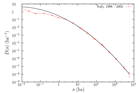
We study in this paper the relation between the temporal properties of forest-fire occurrence and the size of the fires, using the AIB (Archivio Incendi Boschivi) fire catalog compiled by the Italian CFS (Corpo Forestale dello Stato) for all Italy Italy_fire_catalog, covering the years 1998–2002 (included) and containing 36821 fires. In order to characterize the overall behavior, we measure for the whole catalog the probability density of the burned areas $s$ , defined as

D(s)\equiv\frac{\mbox{Prob}[s\leq\mbox{ area }<s+ds]}{ds},

(1)

where $ds$ is the bin size (small enough to sample almost continuously $D(s)$ but large enough to guarantee statistical significance); the resulting shape for $D(s)$ is shown in Fig. 1. Although a power law could be fit to the data, it is clearly seen that the curve is continuously bending downwards, which is the characteristic of a lognormal distribution,

D(s)=\frac{C}{\sqrt{2\pi}\,\sigma s}\,\exp\left(-\frac{\left(\ln s-\mu\right)^{2}}{2\sigma^{2}}\right)\propto\left(\frac{e^{\mu}}{s}\right)^{1+\ \frac{\ln(s/e^{\mu})}{2\sigma^{2}}},

(2)

with $\mu$ and $\sigma$ the mean and standard deviation of $\ln s$ , and $C$ a correction to normalization due to the fact that the fit is not valid for all $s$ . In this way, for each $2\sigma^{2}$ that $\ln s$ is away from $\mu$ the exponent of the previous pseudo-power law increases in one unit (in other words, each decade $s$ is above $e^{\mu}$ increases the exponent in $\ln 10/(2\sigma^{2})$ ). When $s$ is measured in hectares (ha), the results of the best fit yield $\mu=-0.35$ , $\sigma=9.5$ , and $C=6.7$ ; this fit holds not only for the full data but it can be verified that also describes smaller parts of the country and shorter periods of time. In any case, we have no means to conclude if the deviation from a power-law behavior is due to human extinction efforts or to the territorial characteristics of a high-populated country.

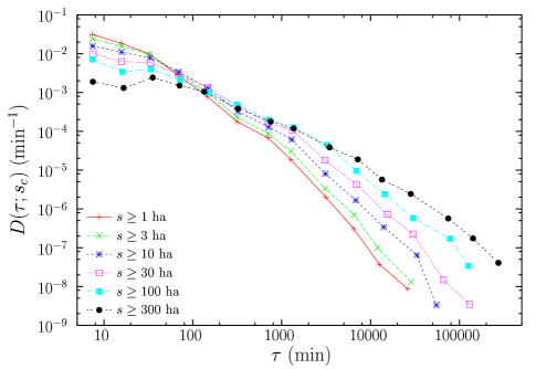
From the distribution of sizes, knowing the total number of events, it is possible to calculate the mean waiting time (or recurrence time) for events above a certain size $s_{c}$ Malamud_fires_pnas; however, looking at the individual values of the waiting times one sees that they are broadly distributed and therefore the mean values are not very informative about the dynamics of the process; so, in order to investigate the temporal properties of fire occurrence it is necessary to look at the whole waiting-time distribution. To be precise, the procedure is as follows: once a spatial area, a time period, and a minimum event size, $s_{c}$ , are selected, the fire history is described as a simple point process, $\{t_{0},t_{1},t_{2}\dots\}$ , where $t_{i}$ denotes the time of occurrence of fire $i$ . For this process, the set of waiting times, defined as the time intervals between consecutive events, is obtained straightforwardly as $\tau_{i}\equiv t_{i}-t_{i-1}.$ Important insight into the nature of the process may be obtained by considering $s_{c}$ not as a constant but as a variable parameter Bak.2002; Corral_prl.2004, and then, the waiting-time probability density for the selected window, defined in the same way as in Eq. (1), will be also considered as a function $D(\tau;s_{c})$ of the minimum size $s_{c}$ .

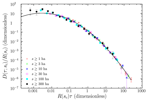
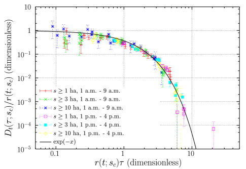
For the whole country and the total temporal extension of the catalog we obtain the different set of curves displayed in Fig. 2(a). We might fit a (decreasing) power law for each distribution, but the exponent would decrease with the increase of the minimum size $s_{c}$ . Instead, it is more convenient to rescale the distributions in order that all of them have the same mean and can be properly compared; this is accomplished by the scale transformation $\tau\rightarrow R(s_{c})\tau$ and $D(\tau;s_{c})\rightarrow D(\tau;s_{c})/R(s_{c})$ , where $R(s_{c})$ is the rate of fire occurrence, defined as the mean number of fires per unit time with $s\geq s_{c}$ (that is, the inverse of the mean of each distribution). The results of the rescaling, as shown in Fig. 2(b), lead to a collapse of the rescaled distributions into a single function $F$ , signaling the fulfillment of a scaling law,

D(\tau;s_{c})=R(s_{c})F(R(s_{c})\tau),

(3)

in the same way as for several natural hazards Corral_prl.2004; Baiesi_flares; Bunde and other avalanche-like processes Yamasaki; Davidsen_fracture.

The rescaled plot unveils more clearly the behavior of the distributions: instead of different power laws, what we have is a unique shape, but at different scales. Again, the apparent continuous decrease of the exponent with the rescaled time, $\theta\equiv R(s_{c})\tau$ , suggest a lognormal shape for $F(\theta)$ as that of Eq. (2), where now we will use tildes to denote the parameters. The best fit yields $\tilde{\mu}=-2.0$ and $\tilde{\sigma}=2.0$ , fixing $\tilde{C}\equiv 1$ . Notice that now we have the constraint that the mean of the rescaled distribution, $\bar{\theta}$ , has to be one; as $\bar{\theta}=e^{\mu+\sigma^{2}/2}$ , this leads to $\mu=-\sigma^{2}/2$ .

It is remarkable that, unlike earthquakes, solar flares, or fractures Corral_prl.2004; Baiesi_flares; Davidsen_fracture; Astrom, forest fires fulfill a scaling law for the waiting time distributions without displaying power-law distribution of event sizes. We could conclude that we have self-similarity in size-time without having scale invariance in size alone. This self-similarity means that for the linear scale transformation $\tau\rightarrow a\tau$ and $s_{c}\rightarrow bs_{c}$ , the value of $b$ which guarantees scale invariance is given by $R(bs_{c})a=R(s_{c})$ , which means that $b$ does not only depend on $a$ , as in the case of a power-law distribution of sizes, but it also depends on $s_{c}$ . This would be equivalent to define an artificial new size variable enforcing that it be power law distributed. However, although this picture describes a kind of self-similarity, it is not a sufficient condition. Indeed, the seasonality of fire occurrence prevents self-similarity in size-time: five years of fire occurrence cannot be equivalent to one year of smaller fires, as there is a clear annual modulation in fire occurrence; nevertheless, for a fixed time window still the small events are a model for the occurrence of the big ones.

Which is then the origin of the scaling law (3)? It is not difficult to relate it with the stationarity of fire sizes and with the existence of a scaling law for the “instantaneous” waiting-time distributions. Indeed, $D(\tau;s_{c})$ is a statistical mixture of those instantaneous waiting-time distributions $D_{t}(\tau;s_{c})$ , which, when the scale of variations of the rate is much larger than the corresponding mean waiting time, take into account that fire occurrence is not stationary but change with time $t$ ; if it is only the instantaneous rate $r(t;s_{c})$ (defined as the number of fires per unit time in a small time interval around $t$ ) what determines fire occurrence, we can write $D_{t}(\tau;s_{c})=D(\tau;s_{c}|r(t;s_{c}))$ and then,

D(\tau;s_{c})=\frac{1}{R(s_{c})}\int_{r_{min}}^{r_{max}}rD(\tau;s_{c}|r)\rho(r;s_{c})\,dr,

where $\rho(r;s_{c})$ is the density of rates, i.e., the fraction of the time the rate is in a particular small range of values, divided by that range Corral_Christensen. Assuming the stationary nature of fire sizes (notice that this is not incompatible with the nonstationarity of time occurrence), this means that $r(t;s_{c})=pr(t;s_{0})$ , where the fraction $p$ is the probability of having a fire larger than $s_{c}$ knowing that it has been larger than $s_{0}$ , $p=\mbox{Prob}[s\geq s_{c}]/\mbox{Prob}[s\geq s_{0}]$ ; this implies that the density of rates fulfills a scaling law, $\rho(r;s_{c})=p^{-1}\rho(p^{-1}r;s_{0})\equiv p^{-1}g(p^{-1}r)$ . Finally, with the hypothesis that $D(\tau;s_{c}|r)$ verifies as well a (instantaneous) scaling law, $D(\tau;s_{c}|r)=rf(r\tau)$ , we get

D(\tau;s_{c})=\frac{1}{pR_{0}}\int_{pa}^{pb}rf(r\tau)p^{-1}g(p^{-1}r)\,dr,

with $r_{min}=pa$ , $r_{max}=pb$ , and $R(s_{c})=pR(s_{0})\equiv pR_{0}$ . A simple change of variables reveals that $D(\tau;s_{c})$ is a function of the form $p\tilde{F}(p\tau)\equiv p\int_{a}^{b}x^{2}f(p\tau x)g(x)dx$ , which is equivalent to the scaling law (3). In other words, if fire occurrence under hypothetical stationary conditions verifies a scaling law for the waiting times (which in this case would be a reflection of the self-similarity of the stationary process, as explained above), non-stationary conditions keep that scaling valid (with a different scaling function) as long as fire size remains stationary and the rate does not become too small for this description to be invalid. [On the other hand, for rates so small that the mean waiting time is much larger than the larger scale of variation of the rate itself (whose existence is not known), the structure of $r(t)$ would become irrelevant and the waiting-time distribution would tend to the exponential form characteristic of Poisson processes.]

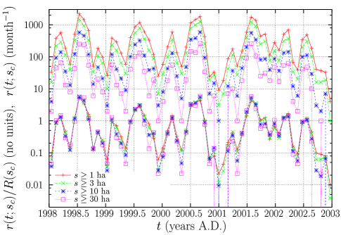
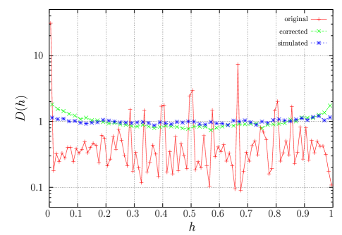
In order to support our argument for the existence of the scaling law (3) we show in Fig. 3 the stationarity of fire sizes, by means of the evolution of $r(t;s_{c})$ for different $s_{c}$ , and how the different curves collapse when they are rescaled by their mean, $R(s_{c})$ ; it is also easy to check that the distribution of rates verifies a scaling law. The last hypothesis, the scaling of $D(\tau;s_{c}|r)$ is more difficult to demonstrate due to the daily oscillations of $r(t;s_{c})$ , which makes that the rate can be considered approximately constant only for a few hours, corresponding to those of the daily maximum and minimum hazard (between 1 p.m. and 4 p.m. and between 1 a.m. and 9 a.m., respectively). This short range of variation leads to very low statistics; nevertheless, for the periods of the year of maximum fire occurrence (for about one month in the summer) the maximum and minimum daily rates are fairly constant for different days, which allows to improve the statistics. The results obtained in this way are shown in Fig. 4, although they are not conclusive. Essentially, they are compatible with an instantaneous scaling law, with perhaps an exponential instantaneous distribution, $D(\tau;s_{c}|r)\simeq re^{-r\tau}$ , but the statistical errors are large; in any case, the hypothesis of the instantaneous scaling law cannot be rejected.

If we find an exponential form for the instantaneous distributions, does this mean that the dynamics can be described by a nonstationary Poisson process? This is the simplest model for nonstationary behavior, for which the events take place at a rate that does not depend on the occurrence of the other events, as in the simple (stationary) Poisson process, but with the difference that the rate changes with time (independently on the process, we can imagine the rate is related to the meteorological conditions, not affected by the presence of fire or not). This leads indeed to exponential instantaneous distributions (provided the rate is not too small), although the reciprocal is not true, in general. If, in addition, the size of the events constitutes an independent random process, this ensures the existence of a scaling law for the instantaneous distributions (as Poisson processes are invariant under random thinning plus rescaling, see Corral_prl.2005). The nonstationary Poisson process has been recently used for earthquake occurrence, see Ref. Shcherbakov.

A test to verify if a process is of the nonstationary Poisson type was introduced by Bi et al. Bi. One only needs to compute for each $i$ the statistics $h_{i}\equiv 2\tau_{{min}\,i}/(2\tau_{{min}\,i}+\tau_{{neig}\,i})$ , where $\tau_{{min}\,i}$ is the minimum of $\tau_{i}$ and $\tau_{i+1}$ , and $\tau_{{neig}\,i}$ is the length of the interval neighbor of the minimum one opposite to the one used in the comparison, i.e., $\tau_{i-1}$ or $\tau_{i+2}$ respectively. Under the hypothesis we want to test, both $\tau_{{neig}}$ and $2\tau_{{min}}$ are independent and exponentially distributed with approximately the same rate, $r(t)$ , and therefore it can be shown that $h$ is uniformly distributed between 0 and 1.

The application of the test to the fire data yields catastrophic results, see Fig. 5. The obtained probability density for $h$ is far from uniform, with very large peaks for precise $h$ -values. This is due to the discretization of fire occurrences in the catalog, which are determined verbally and therefore rounded mainly in units of 10 or 15 min; this favors particular values of $\tau$ and there fore of $h$ (2/3, 4/5, 1/2, etc.). We can correct this effect by the addition of a uniform random value between -5 min and 5 min to each occurrence time $t_{i}$ , then the peaks in the distribution of $h$ disappear and its shape gets closer to a uniform one; however, the difference is significant. We have verified that the difference is not due to the random addition we have performed: simulation of a non-stationary Poisson process where the occurrences are rounded in intervals of 10 min yields a perfect uniform distribution when this discretization is corrected by the uniform random addition just explained (Fig. 5). In consequence, this model does not seem suitable for fire occurrence, and although the instantaneous distributions are close to exponential (Fig. 4), this is not a sufficient condition to have a nonstationary Poisson process, as the absence of correlations is equally important for it.

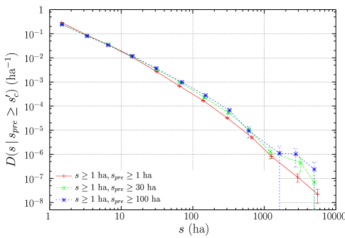
If we reject the nonstationary Poisson process with independent sizes as a model of fire occurrence, the only way to get a scaling law for the instantaneous process is by means of orchestrated correlations between sizes and occurrence times Corral_prl.2005. In order to establish the existence of such correlations we proceed to study conditional size distributions, defined as in Eq. (1) but with an additional condition for the computation of the probability. We consider $D(s\,|\,s_{pre}\geq s_{c}^{\prime})$ , which accounts for the size of the events for which the size of the immediate previous-in-time event, $s_{pre}$ , is above a given threshold $s_{c}^{\prime}$ . The results in Fig. 6 show that an increase of $s_{c}^{\prime}$ triggers a greater proportion of large fires, i.e., large fires are followed by large fires. The dependence of a fire size on the previous size is small but significant, unlike to what happens for earthquakes, where correlation between their magnitudes has not been detected Corral_comment; Corral_tectono (nevertheless, for an alternative view see Ref. Lippiello). On the other hand, the dependence of waiting times on the size of the event defining the starting of the waiting period can be measured by $D(\tau;s_{c}\,|\,s_{pre}\geq s_{c}^{\prime})$ showing how large fires cause a decrease in the number of long recurrence times, i.e., those fires tend to be closer in time to the next fires. The effect is again small, but clearly detectable, and in this case has a counterpart for earthquakes, where the Omori law for aftershocks implies the same behavior.

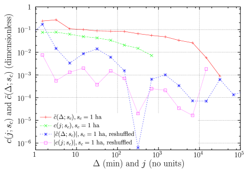
But the correlations between fires are not only with the previous event; its range can be quantified by means of the following auto-correlation function,

c(j;s_{c})=\left\langle(\log s_{i}-\bar{\ell})(\log s_{i+j}-\bar{\ell})\right\rangle\sigma_{\ell}^{-2},

where $\bar{\ell}$ is the arithmetic mean of the logarithm of the size (i.e., the logarithm of the geometric mean of the size), and $\sigma_{\ell}$ is the standard deviation of the logarithm; both $\ell$ and $\sigma_{\ell}$ depend on $s_{c}$ . Notice that although the process is not stationary, the stationarity of the size gives sense to the autocorrelation function defined in this way. The results for this function are shown in Fig. 7, and compared with the same correlation function calculated for a reshuffled version of the catalog, for which the size of the events are randomly permuted, breaking the correlations between them (which should yield an autocorrelation function fluctuation around zero). The conclusion is that positive correlations extend significantly beyond several hundreds of events (for events of size larger than 1 ha).

More clear is the behavior of the autocorrelation as a function of time; as the process is not stationary both functions are not equivalent. We define

\tilde{c}(\Delta;s_{c})=\left\langle(\log s(t)-\bar{\ell})(\log s(t+\Delta)-\bar{\ell})\right\rangle\sigma_{\ell}^{-2},

where $s(t)$ denotes the size of the fire that happens at time $t$ (we slightly change notation, for convenience). The average is taken over all times $t$ and $t+\Delta$ for which there are fires, this yields the results of Fig. 7. The correlation is again positive, but larger in this case, suggesting that real time is a better variable to describe the evolution of correlations, which extend for about 10000 min, i.e., roughly 1 week. It is likely that these correlations are mediated through the meteorological conditions.

In summary, the dynamics of forest-fire occurrence shows a complex scale-invariant structure at any time, modulated by seasonal and daily variations and orchestrated by means of broad-range correlations.

Scaling and correlations in the dynamics of forest-fire occurrence

Abstract