Concise theory of chiral lipid membranes

Abstract

A theory of chiral lipid membranes is proposed on the basis of a concise free energy density which includes the contributions of the bending and the surface tension of membranes, as well as the chirality and orientational variation of tilting molecules. This theory is consistent with the previous experiments [J.M. Schnur et al., Science 264, 945 (1994); M.S. Spector et al., Langmuir 14, 3493 (1998); Y. Zhao, et al., Proc. Natl. Acad. Sci. USA 102, 7438 (2005)] on self-assembled chiral lipid membranes of DC_8,9PC. A torus with the ratio between its two generated radii larger than $\sqrt{2}$ is predicted from the Euler-Lagrange equations. It is found that tubules with helically modulated tilting state are not admitted by the Euler-Lagrange equations, and that they are less energetically favorable than helical ripples in tubules. The pitch angles of helical ripples are theoretically estimated to be about 0^∘ and 35^∘, which are close to the most frequent values 5^∘ and 28^∘ observed in the experiment [N. Mahajan et al., Langmuir 22, 1973 (2006)]. Additionally, the present theory can explain twisted ribbons of achiral cationic amphiphiles interacting with chiral tartrate counterions. The ratio between the width and pitch of twisted ribbons is predicted to be proportional to the relative concentration difference of left- and right-handed enantiomers in the low relative concentration difference region, which is in good agreement with the experiment [R. Oda et al., Nature (London) 399, 566 (1999)].

I Introduction

Since tubules were fabricated successfully from chiral lipid molecules, chiral lipid structures have attracted much experimental attention Schnur93 ; Schnur94 ; Spector98 ; Zhaoy05 ; Zhaoy06 ; Spector01 ; Chung93 ; Zastavker ; Oda99 ; Oda02 . Most of chiral structures in experiments are self-assembled from DC${}_{8,9}PC$ which is a typical chiral molecule. Schnur et al. have observed that the spherical vesicles in solution have very weak circular dichroism signal while tubules have strong one Schnur94 . Spector et al. have investigated the chiral lipid tubules formed from various proportions of left- and right-handed DC${}_{8,9}PC$ molecules and found that they are of similar radii Spector98 , which reveals that the radii of chiral tubules do not depend on the strength of the molecular chirality. Fang’s group has carefully resolved the molecular tilting order in the tubules and concluded that the projected direction of the molecules on the tubular surfaces departs 45^∘ from the equator of the tubules at the uniform tilting state Zhaoy05 . Helical ripples in lipid tubules are also observed by the same group with atomic force microscopy Zhaoy06 . Their pitch angles are found to be concentrated on about 5^∘ and 28^∘ Zhaoy06 . Cholesterol is another kind of chiral molecules used in the experiments where helical stripes with pitch angles $11^{\circ}$ and $54^{\circ}$ are usually observed Chung93 ; Zastavker . Additionally, Oda et al. have reported twisted ribbons of achiral cationic amphiphiles interacting with chiral tartrate counterions Oda99 ; Oda02 . It is found that the twisted ribbons can be tuned by the introduction of opposite-handed chiral counterions in various proportions Oda99 . From the experimental data Oda99 , we see that the ratio between the width and pitch of the ribbons is proportional to the relative concentration difference of left- and right-handed enantiomers in the low relative concentration difference region. Can we interpret all or at least most of above experimental results within a unified theory?

There are several theoretical discussions on chiral lipid membranes (CLMs) in the previous literature, where the chiral molecules are assumed to be in a Smectic C^∗ phase at which the direction of the molecules is tilted from the normal of the membranes at a constant angle. The possible free energy of CLMs is discussed by Helfrich and Prost from symmetry arguments Helfrich88 . Their theory has been further developed and applied in many studies oy90 ; Nelson92 ; Selinger93 ; Selinger96 ; Selinger01 ; oy98 ; HuLo05 . Nelson and Powers have investigated the thermal fluctuations of CLMs Nelson92 . Selinger et al. have discussed tubules with helically modulated tilting state and helical ripples in tubules Selinger93 ; Selinger96 ; Selinger01 . Komura and Ou-Yang have given an explanation to the high-pitch helical stripes of cholesterol molecules oy98 . Due to the complicated form of the free energy used in these theories Helfrich88 ; oy90 ; Nelson92 ; Selinger93 ; Selinger96 ; Selinger01 ; oy98 , it is almost impossible to obtain the general Euler-Lagrange equations corresponding to the free energy. Thus one cannot determine whether a configuration, such as a twisted ribbon, a tubule with helically modulated tilting state or a helical stripe, is a true equilibrium structure or not. This difficulty was always ignored in previous discussion of both tubules with helically modulated tilting state and helical stripes Selinger93 ; Selinger96 ; Selinger01 ; oy98 . Can we confront this difficulty and construct a more concise theory of CLMs consistent with the experiments, in which we can unambiguously say which configuration is a genuine equilibrium structure?

We will address these questions in this paper, which is organized as follows: In Sec. II, we introduce a concise free energy density of CLMs which includes the contributions of the bending and the surface tension of the membranes, as well as the chirality and orientational variation of the tilting molecules. In Sec. III, we present the Euler-Lagrange equations for CLMs without free edges and use them to explain experimental data Schnur94 ; Spector98 ; Zhaoy05 ; Zhaoy06 . We predict a torus with the ratio between its two generated radii larger than $\sqrt{2}$, which has not yet been observed in the experiments on self-assembled CLMs. In Sec. IV, we present the Euler-Lagrange equations and boundary conditions for CLMs with free edges and use them to discuss experimental data Chung93 ; Zastavker ; Oda99 . Sec. V is a brief summary and discussion. In the Appendixes, we briefly derive the Euler-Lagrange equations for CLMs without free edges and the Euler-Lagrange equations as well as boundary conditions for CLMs with free edges through the variational method tzcjpa developed by one of the present authors. Several mathematical details are also put in the Appendixes.

II Free energy density

Following the above theories Helfrich88 ; oy90 ; Nelson92 ; Selinger93 ; Selinger96 ; Selinger01 ; oy98 , we adopt a concise form of free energy density for a CLM which consists of the following contributions.

(i) The bending and surface energy per area is taken as Helfrich’s form helfrich

$$G_{H}=(k_{c}/2)(2H+c_{0})^{2}-\bar{k}K+\lambda,$$ (1)

where $k_{c}$ and $\bar{k}$ are bending rigidities, and $\lambda$ the surface tension. $c_{0}$ is the spontaneous curvature reflecting the asymmetrical factors between two sides of the membrane. $H$ and $K$ are the mean curvature and Gaussian curvature of the membrane, respectively, which can be expressed as $2H=-(1/R_{1}+1/R_{2})$, $K=1/R_{1}R_{2}$ by the two principal curvature radii $R_{1}$ and $R_{2}$. The curvature energy in Eq. (1) is invariant under the coordinate rotation around the normal of the membrane surface, but will change under the inversion of the normal if $c_{0}\neq 0$.

(ii) The energy per area originating from the chirality of tilting molecules has the form oy90

$$G_{ch}=-h\tau_{\mathbf{m}},$$ (2)

where $h$ reflects the strength of the molecular chirality which usually determines the handedness of CLMs—the CLMs with the opposite handedness will be observed in experiments if $h$ changes its sign Schnur94 . Without losing the generality, we only discuss the case of $h>0$ in this paper. $\tau_{\mathbf{m}}$ is the geodesic torsion along the unit vector $\mathbf{m}$ at some point. Here $\mathbf{m}$ represents the projected direction of the lipid molecules in the experiments Schnur94 ; Spector98 ; Zhaoy05 ; Zhaoy06 ; Spector01 ; Chung93 ; Zastavker and chiral tartrate counterions in the experiment Oda99 ; Oda02 on the membrane surface, respectively. If we take a right-handed orthonormal frame $\{\mathbf{e}_{1},\mathbf{e}_{2},\mathbf{e}_{3}\}$ with $\mathbf{e}_{3}$ being the normal vector of the membrane as shown in Fig. 1, $\mathbf{m}$ can be expressed as $\mathbf{m}=\cos\phi\mathbf{e}_{1}+\sin\phi\mathbf{e}_{2}$, where $\phi$ is the angle between $\mathbf{m}$ and $\mathbf{e}_{1}$. At this frame, the curvature tensor can be expressed as a matrix with element $a$, $b$, and $c$ shown in Appendix A. With the curvature tensor, the geodesic torsion along $\mathbf{m}$ can be expressed as tzcjpa

$$\tau_{\mathbf{m}}=b(\cos^{2}\phi-\sin^{2}\phi)+(c-a)\cos\phi\sin\phi,$$ (3)

which is the same as the chiral term in the previous literature, such as the last term of Eq. (2) in Ref. Helfrich88 , Eq. (3) in Ref. Nelson92 , and the third term of Eq. (2.1) in Ref. Selinger96 . In particular, for the principal frame, the above equation is simplified as

$$\tau_{\mathbf{m}}=(1/R_{1}-1/R_{2})\cos\phi\sin\phi.$$ (4)

We will confine $\phi$ to the region ($-\pi/2,\pi/2$] because of the relation $\tau_{\mathbf{m}}(\phi+\pi)=\tau_{\mathbf{m}}(\phi)$. Moreover, it is easy to see that the geodesic torsion along the mirror image of $\mathbf{m}$ with respect to $\mathbf{e}_{1}$ changes its sign because $\phi\mapsto-\phi$ under the reflection with respect to $\mathbf{e}_{1}$. Thus this term breaks the inversion symmetry in the tangent plane at each point of the membrane, which allows us to distinguish the handedness. Additionally, from Eq. (4) we can see that the minimum of Eq. (2),

$$G_{ch}^{min}=-(h/2)|1/R_{1}-1/R_{2}|,$$ (5)

is reached when $\mathbf{m}$ departs from the principal direction at a angle $+\pi/4$ or $-\pi/4$ for a given shape of the membrane. Here the sign in front of $\pi/4$ depends on the sign of $(1/R_{1}-1/R_{2})$. The larger difference between $R_{1}$ and $R_{2}$ is, the larger absolute value of $G_{ch}^{min}$ is reached. In other words, the chiral term favors saddle surfaces (for example, the twisted ribbons in Sec. IV.3) whose two principal curvature radii $R_{1}$ and $R_{2}$ have opposite signs.

Figure 1: Right-handed orthonormal frame $\{\mathbf{e}_{1},\mathbf{e}_{2},\mathbf{e}_{3}\}$ at any point in a surface where $\mathbf{e}_{3}$ is the normal vector of the surface. (A) Surface without boundary curve. (B) Surface with boundary curve where $\mathbf{t}$ is the tangent vector of the boundary curve, and $\mathbf{b}$, in the tangent plane of the surface, is perpendicular to $\mathbf{t}$.

(iii) The energy per area due to the orientational variation of $\mathbf{m}$ is taken as Lubensky92

$$G_{ov}=(k_{f}/2)[(\nabla\times\mathbf{m})^{2}+(\nabla\cdot\mathbf{m})^{2}],$$ (6)

where $k_{f}$ is a constant in the dimension of energy. This is the simplest term of energy cost due to tilting order invariant under the coordinate rotation around the normal of the membrane surface. $\nabla$ is the 2-dimensional (2D) gradient operator on the membrane surface, and the 2D cross product “$\times$” gives a scalar. By defining a spin connection field $\mathbf{S}$ satisfying $\nabla\times\mathbf{S}=K$ Nelson87 , one can derive

$$(\nabla\times\mathbf{m})^{2}+(\nabla\cdot\mathbf{m})^{2}=(\nabla\phi-\mathbf{S})^{2}$$ (7)

through simple calculations.

The total free energy density adopted in the present paper, $G=G_{H}+G_{ch}+G_{ov}$, has the following concise form:

$$G=\frac{k_{c}}{2}(2H+c_{0})^{2}-\bar{k}K+\lambda-h\tau_{\mathbf{m}}+\frac{k_{f}}{2}\mathbf{v}^{2},$$ (8)

where $\mathbf{v}\equiv\nabla\phi-\mathbf{S}$. This special form might arguably be the most natural and concise construction including the bending, chirality and tilting order, for the given vector field $\mathbf{m}$ and normal vector field $\mathbf{e}_{3}$. Of course, using these two fields, one can also construct more general free energy densities which contain much more terms Helfrich88 ; oy90 ; Nelson92 ; Selinger93 ; Selinger96 ; Selinger01 ; oy98 . Compared with the general form, our special form is simplified in two aspects: (i) The contributions of the bending of membranes and the orientational elasticity of $\mathbf{m}$ are taken as the isotropic forms; (ii) There is no additional coupling between $\mathbf{m}$ and the curvature of membranes except the chiral term (2), which makes it a concise theory. Although our free energy density is not new relative to the general form appearing in the previous literature, we derive for the first time the corresponding Euler-Lagrange equations without any assumption on the shapes of membranes before doing the variation, and then check which configuration solves the Euler-Lagrange equations. More importantly, in the following, we will see that most of the experimental results can be explained in terms of such a concise free energy density.

III Chiral lipid membranes without free edges

CLMs without free edges usually correspond to closed vesicles. Here a long enough tubule, where the end effect is neglected, is also regarded as a CLM without free edges. In this section, we show the Euler-Lagrange equations of CLMs without free edges (derived briefly in Appendix B), and then discuss CLMs in spherical, tubular and torus shapes. As we will see, our theoretical results are in good agreement with the experiments Schnur94 ; Spector98 ; Zhaoy05 ; Zhaoy06 .

III.1 Euler-Lagrange equations

The free energy for a closed CLM can be expressed as

$$F=\int G\ dA+P\int dV,$$ (9)

where $dA$ is the area element of the membrane and $dV$ the volume element enclosed by the vesicle. $P$ is either the pressure difference between the outer and inner sides of the vesicle or used to implement a volume constraint. For tubular configuration, we usually take $P=0$.

Using the variational method tzcjpa , we obtain the Euler-Lagrange equations corresponding to the free energy (9) as

$$2h(\kappa_{\mathbf{m}}-H)-k_{f}\nabla^{2}\phi=0,$$ (10)

and

$$2k_{c}\nabla^{2}H+k_{c}(2H+c_{0})(2H^{2}-c_{0}H-2K)-2\lambda H+P$$

$$+h[\nabla\cdot(\mathbf{m}\nabla\times\mathbf{m})+\nabla\times(\mathbf{m}\nabla\cdot\mathbf{m})]$$

$$+k_{f}[(\kappa_{\mathbf{v}}-H)\mathbf{v}^{2}-\nabla\mathbf{v}\colon\nabla\mathbf{e}_{3}]=0,$$ (11)

where $\kappa_{\mathbf{m}}$ and $\kappa_{\mathbf{v}}$ are the normal curvature along the directions of $\mathbf{m}$ and $\mathbf{v}$, respectively. They can be expressed as Eqs. (55) and (56) with the curvature tensor. Physically, Eqs. (10) and (11) express the moment and force balances along the normal $\mathbf{e}_{3}$ at each point of the membrane. If $h$ and $k_{f}$ vanish, the above two equations degenerate into the shape equation of achiral lipid vesicles, which has been fully discussed in Refs. oy87 ; Lipowsky91 ; Seifert97 ; oybook ; DuLiuWang06 .

Two remarks are necessary concerning Eq. (10): (i) We have selected the proper gauge such that $\nabla\cdot\mathbf{S}=0$, or else $\nabla^{2}\phi$ should be replaced with $\nabla^{2}\phi-\nabla\cdot\mathbf{S}$. (ii) For closed vesicles different from toroidal topology, the tangent vector field $\mathbf{m}$ will have singular points. In this case, the right-hand term should be replaced with the sum of $\delta$-function, $\sum_{i}\sigma_{i}\delta(\mathbf{r}-\mathbf{r}_{i})$, where $\mathbf{r}$ and $\mathbf{r}_{i}$ represent any point and singular point in the CLM, while $\sigma_{i}$ represents the strength of the source or vortex at the singular point $\mathbf{r}_{i}$.

III.2 Spherical vesicles

For spherical vesicles of chiral lipid molecules, $\tau_{\mathbf{m}}$ is always vanishing because $R_{1}=R_{2}$. Thus the free energy (9) is independent of the molecular chirality and permits the same probability of left- and right-handed spherical vesicles existing in solution. Naturally, no evident circular dichroism signal would be observed, which is consistent with the experiment Schnur94 . Of course, we cannot exclude the other possible explanation of this experiment that the lipid molecules are non-tilting in the spherical vesicles Selinger01 .

III.3 Tubules with uniform tilting state

A tubule is regarded as an cylinder with radius $\rho$ and infinite length. Then $H=-1/2\rho$, $\kappa_{\mathbf{m}}=-\cos^{2}\phi/\rho$, and $\tau_{\mathbf{m}}=\sin 2\phi/2\rho$, where $\phi$ is the angle between $\mathbf{m}$ and the equator of the cylinder. $\phi$ is a constant for the tubule with the uniform tilting state as shown in Fig. 2(a). Thus Eq. (10) requires

$$\phi=\pm\pi/4.$$ (12)

We should keep $\phi=\pi/4$ because it corresponds to the local minimum of $-h\int\tau_{\mathbf{m}}dA$, which is in good agreement with the experiment by Fang’s group Zhaoy05 where the projected direction of the molecules on the tubular surfaces indeed departing 45^∘ from the equator of the tubules with the uniform tilting state.

For the cylindrical shape, we set $P=0$. It is easy to find $\nabla\cdot(\mathbf{m}\nabla\times\mathbf{m})+\nabla\times(\mathbf{m}\nabla\cdot\mathbf{m})$ and $(\kappa_{\mathbf{v}}-H)\mathbf{v}^{2}-\nabla\mathbf{v}\colon\nabla\mathbf{e}_{3}$ both to be vanishing for $\phi=\pi/4$. Thus Eq. (11) is transformed into

$$k_{c}(c_{0}^{2}\rho^{2}-1)+2\lambda\rho^{2}=0.$$ (13)

This equation indicates that the radius $\rho$ of chiral lipid tubules is independent of the strength of molecular chirality $h$, which is consistent with the experiment Spector98 where the tubular radius is insensitive to the proportion of left- and right-handed DC${}_{8,9}PC$ in the tubule. However, we cannot exclude the other possible explanation that DC${}_{8,9}PC$ molecules with different handedness are not mixed in the tubule such that each tubule in solution contains merely the one kind of molecules with the same handedness ether left- or right-handed Spector98 ; Selinger01 .

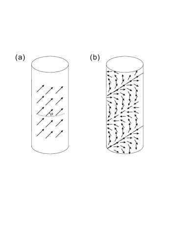
Figure 2: Tubules: (a) Uniform tilting state; (b) Helically modulated tilting state. Arrows represent the projected directions $\{\mathbf{m}\}$ of the tilting molecules on the tubules.

III.4 Tubules with helically modulated tilting state

The concept of tubules with helically modulated tilting state was proposed by Selinger et al. Selinger96 . The orientational variation of the tilting molecules is assumed to be linear and confined to a small range. Here we will directly investigate the orientational variation by using the Euler-Lagrange equation (10) without this assumption. Additionally, as mentioned in the Introduction, whether the tubules with helically modulated titling state are equilibrium configurations or not is not addressed in Ref. Selinger96 . However, our theory will unambiguously reveal that they are not equilibrium configurations. Let $s$ and $z$ denote the arc length parameters along the circumferential and axial directions, respectively. If $\phi$, the angle between $\mathbf{m}$ and the equator of the cylinder, is not a constant, Eqs. (10) and (11) are then transformed into

$$k_{f}(\phi_{ss}+\phi_{zz})+(h/\rho)\cos 2\phi=0,$$ (14)

and

$$h[2(\phi_{z}^{2}-\phi_{s}^{2}+\phi_{sz})\sin 2\phi+(\phi_{ss}-\phi_{zz}+4\phi_{z}\phi_{s})\cos 2\phi]$$

$$+\lambda/\rho+k_{c}(c_{0}^{2}-1/\rho^{2})/2\rho+k_{f}[(\phi_{z}^{2}-\phi_{s}^{2})/2\rho+\phi_{sz}/\rho]$$

$$=0.$$ (15)

where the subscripts $s$ and $z$ represent the partial derivatives respect to $s$ and $z$, respectively. The derivations of the above two equations are shown in Appendix D.

At the helically modulated tilting state, $\phi$ is invariant along the direction of a fictitious helix enwinding around the tubule as shown in Fig. 2(b). Let $\psi$ be the pitch angle of that helix and apply a coordinate transformation $(s,z)\rightarrow(\zeta,\eta)$ via $\zeta=s\cos\psi+z\sin\psi,\eta=-s\sin\psi+z\cos\psi$, where $\zeta$ is the coordinate along the helix and $\eta$ is the coordinate orthogonal to $\zeta$. In the new coordinates, $\phi$ depends only on $\eta$. Changing variable $\Theta=\phi-\psi$ and introducing the dimensionless parameters $\chi=\eta/\rho$ and $\bar{h}=h\rho/k_{f}$, we transform Eqs. (10) and (11), respectively, into

$$\Theta_{\chi\chi}=-\bar{h}\cos 2(\Theta+\psi),$$ (16)

and

$$(k_{c}/k_{f})(1-c_{0}^{2}\rho^{2})-2\lambda\rho^{2}/k_{f}=R,$$ (17)

where $R\equiv\Theta_{\chi}^{2}\cos 2\psi-\Theta_{\chi\chi}\sin 2\psi+2\bar{h}(2\Theta_{\chi}^{2}\sin 2\Theta-\Theta_{\chi\chi}\cos 2\Theta)$.

The first integral of Eq. (16) is

$$\Theta_{\chi}^{2}=\mu^{2}-\bar{h}\sin 2(\Theta+\psi),$$ (18)

with an unknown constant $\mu$. Substituting Eqs. (16) and (18) into Eq. (17), we obtain the right-hand side of Eq. (17):

$$R = \mu^{2}\cos 2\psi+\bar{h}(4\mu^{2}-1)\sin 2\Theta$$ (19)

$$+ 2\bar{h}^{2}[\cos(4\Theta+2\psi)-\sin 2\Theta\sin 2(\Theta+\psi)].$$

The necessary condition for validity of Eq. (17) is that the right-hand side $R$ is constant, which, in terms of Eq. (19), holds if and only if $\bar{h}=0$ for varying $\Theta$. Therefore, tubules with helically modulated tilting state are not admitted by the Euler-Lagrange equation (11) if $h\neq 0$. In other words, the orientational variation of the tilting lipid molecules breaks the force balance along the normal direction of the tubule at this state, which might rather induce helical ripples in tubules.

III.5 Helical ripples in tubules

Assume now that a tubule with radius $\rho$ undergoes small out-of-plane deformations and reaches a new configuration expressed as a vector $\{\rho(1+y)\cos(s/\rho),\rho(1+y)\sin(s/\rho),z\}$, where $|y|\ll 1$ is a function of $s$ and $z$. For simplicity, we take $c_{0}=0$, $\lambda=0$, $k_{f}\simeq k_{c}$, and $\bar{h}\ll 1$ in this subsection. As shown in Appendix E, Eqs. (10) and (11) can be transformed into

$$\rho^{2}(\phi_{ss}+\phi_{zz}+\phi_{z}y_{z}-\phi_{s}y_{s}-2y\phi_{ss}-y_{zs})=-\bar{h}\cos 2\phi$$ (20)

and

$$(k_{c}/k_{f}\rho^{2})[(1+\rho^{2}\partial_{ss}+\rho^{2}\partial_{zz})^{2}y-1/2]$$

$$+(k_{c}/k_{f}\rho^{2})[(1+\rho^{2}\partial_{ss}+\rho^{2}\partial_{zz})y/2-2\rho^{2}y_{zz}]$$

$$+\bar{h}[2(\phi_{z}^{2}-\phi_{s}^{2}+\phi_{sz})\sin 2\phi+(\phi_{ss}-\phi_{zz}+4\phi_{z}\phi_{s})\cos 2\phi]$$

$$+(\phi_{s}^{2}-\phi_{z}^{2})(y+\rho^{2}y_{ss}-\rho^{2}y_{zz}-1)/2$$

$$+\phi_{sz}+y\phi_{s}^{2}-2y\phi_{sz}-y_{zz}+2\rho^{2}y_{sz}\phi_{s}\phi_{z}=0,$$ (21)

where $\phi$ is the angle between $\mathbf{m}$ and the equator of the tubule.

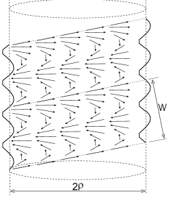
Figure 3: Small amplitude ripples in a tubule with radius $\rho$. Arrows represent the projected directions $\{\mathbf{m}\}$ of the tilting molecules on the ripples’ surface.

Now we consider helical ripples in the tubule where $\phi$ and $y$ are invariant along the direction of a fictitious helix enwinding around the tubule as shown in Fig. 3. We adopt the same coordinate transformation as the above subsection, and let $\vartheta=\phi-(\Theta+\psi)$, where $\psi$ is the pitch angle of the fictitious helix and $\Theta$ is governed by Eq. (16). Then the above equations (20) and (21) are reduced to a matrix equation

$$\mathcal{L}\Psi=\Phi,$$ (22)

with $\Psi\equiv\{\vartheta,y\}^{t}$ and $\Phi\equiv\{0,(\bar{h}/2)(1-4\mu^{2})\sin 2\Theta\}^{t}$, where the superscript ‘$t$’ represents the transpose. The differential operator $\mathcal{L}$ has four matrix elements:

$$\mathcal{L}_{11}\equiv-{d^{2}}/{d\chi^{2}},$$

$$\mathcal{L}_{12}\equiv-\mu\cos 2\psi{d}/{d\chi}-\sin\psi\cos\psi{d^{2}}/{d\chi^{2}},$$

$$\mathcal{L}_{21}\equiv\mu\cos 2\psi{d}/{d\chi}-\sin\psi\cos\psi{d^{2}}/{d\chi^{2}},$$

$$\mathcal{L}_{22}\equiv\mu^{2}\cos^{2}\psi+\mu^{2}\cos 2\psi{d^{4}}/{d\chi^{4}}$$

$$\hskip 18.49428pt+[2\mu^{2}\cos 2\psi\sin^{2}\psi+(\mu^{2}-1)\cos^{2}\psi]{d^{2}}/{d\chi^{2}},$$

where $\mu$ satisfies

$$\mu^{2}\cos 2\psi=k_{c}/k_{f}.\\$$ (23)

It is not hard to find a special solution of Eq. (22) as

$$\tilde{\Psi}=\frac{\bar{h}(1-4\mu^{2})}{4\Gamma}\left(\begin{array}[]{l}\cos 2(\Theta+\psi)\\ 2\sin 2\Theta\end{array}\right)$$ (24)

with $\Gamma\equiv\mu^{2}(3\cos^{2}\psi+\cos 2\psi-8\mu^{2}\cos 2\psi\sin^{2}\psi-4\mu^{2}\cos^{2}\psi+16\mu^{4}\cos 2\psi)$. Considering Eq. (23), we can prove $\Gamma>0$ for $k_{c}/k_{f}>0.133$ and hence $\Gamma>0$ for $k_{c}\simeq k_{f}$.

Note that Eq. (22) contains only the first order terms of $\vartheta$ and $y$, which can also be obtained from the variation of the free energy $F$ expanded up to the second order terms of $\vartheta$ and $y$. The dimensionless mean energy difference between the tubule with helical ripples and that with helically modulated tilting state is expressed as

$$\Delta F=\int_{0}^{W/\rho}\left(\frac{1}{2}\Psi^{t}\mathcal{L}\Psi-\Psi^{t}\Phi\right)d\chi,$$ (25)

where $W$ is the period of the ripples along $\eta$ direction as show in Fig. 3. Substituting the solution (24) into the above equation, we have

$$\Delta F=-\frac{\bar{h}^{2}(1-4\mu^{2})^{2}}{8\Gamma}\int_{0}^{W/\rho}\sin^{2}2\Theta d\chi<0,$$ (26)

which reveals that a tubule with ripples is energetically more favorable than that in a helically modulated titling state. Additionally, we can easily prove from Eq. (23) that the pitch angle obeys $\psi<45^{\circ}$. All ripples in tubules resolved in the recent experiment Zhaoy06 with atomic force microscope have indeed the pitch angles smaller than $45^{\circ}$. The tubules with ‘helically modulated tilting state’ observed in the experiment Lvov might also be the tubules with helical ripples whose amplitudes are below the experimental resolution. In this experiment, all pitch angles are also smaller than $45^{\circ}$.

Considering $\bar{h}\ll 1$, we have $\Theta_{\chi}\approx\mu$ from Eq. (18) and then

$$\mu W/\rho\approx 2\pi,$$ (27)

due to $W$ being the period of the ripples along $\eta$ direction. If the pitch angle $\psi=0$, the fictitious helix is a circle, and Eqs. (23) and (27) requires $2\pi\rho/W\approx\sqrt{k_{c}/k_{f}}$. If $\psi\neq 0$, the fictitious helix is indeed a helix satisfying $W=2\pi\rho\sin\psi$. It is then easy to derive

$$\cos 2\psi/\sin^{2}\psi\approx k_{c}/k_{f}$$ (28)

from Eqs. (23) and (27). Therefore, two kinds of ripples are permitted in our theory: one has pitch angle about $0^{\circ}$; another satisfies Eq. (28), which gives $\psi\simeq 35^{\circ}$ for $k_{c}\simeq k_{f}$. Our theoretical results are thus close to the most frequent pitch angles (about 5^∘ and 28^∘) of the ripples in tubules observed by Fang’s group Zhaoy06 .

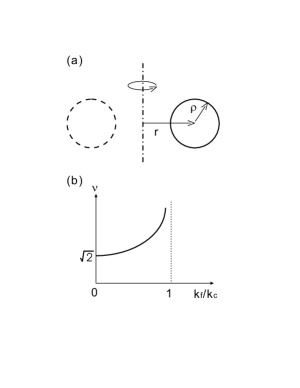
Figure 4: (a) Torus generated by a cycle rotating around an axis in the same plane of the cycle. (b) Ratio of the generated radii ($\nu$), Eq. (31), as a function of $k_{c}/k_{f}$.

III.6 Torus, a prediction

A torus is a revolution surface generated by a cycle with radius $\rho$ rotating around an axis in the same plane of the cycle as shown in Fig. 4(a). The revolution radius $r$ should be larger than $\rho$. A point in the torus can be expressed as a vector $\{(r+\rho\cos\varphi)\cos\theta,(r+\rho\cos\varphi)\sin\theta,\rho\sin\varphi\}$. As shown in Appendix F, Eq. (10) is transformed into

$$\frac{\phi_{\theta\theta}}{\nu+\cos\varphi}+[(\nu+\cos\varphi)\phi_{\varphi}]_{\varphi}-\frac{\nu h\rho}{k_{f}}\cos 2\phi=0,$$ (29)

where $\phi$ is the angle between $\mathbf{m}$ and the latitude of the torus, while

$$\nu\equiv r/\rho$$

is the ratio between two generated radii of the torus.

It is found that the uniform tilting state $\phi=-\pi/4$ satisfies the above equation (29) and that makes $-\int h\tau_{\mathbf{m}}dA$ to take the minimum by considering Eq. (121). As shown in Appendix F, with $\phi=-\pi/4$, Eq. (11) is transformed into

$$(2k_{c}-k_{f})/{\nu^{2}}+k_{c}(c_{0}^{2}\rho^{2}-1)+2(P\rho+\lambda)\rho^{2}$$

$$+\frac{4k_{c}c_{0}^{2}\rho^{2}-4k_{c}c_{0}\rho-2h\rho+8\lambda\rho^{2}+6P\rho^{3}}{\nu}\cos\varphi$$

$$+\frac{5k_{c}c_{0}^{2}\rho^{2}-8k_{c}c_{0}\rho-4h\rho+10\lambda\rho^{2}+3k_{f}+6P\rho^{3}}{\nu^{2}}\cos^{2}\varphi$$

$$+\frac{2k_{c}c_{0}^{2}\rho^{2}-4k_{c}c_{0}\rho-2h\rho+4\lambda\rho^{2}+2k_{f}+2P\rho^{3}}{\nu^{3}}\cos^{3}\varphi$$

$$=0.$$ (30)

If $\nu\rightarrow\infty$ and $P=0$, the above equation degenerates into Eq. (13) obeyed by a tubule with radius $\rho$ at uniform tilting state. If $\nu$ is finite, then Eq. (30) holds if and only if the coefficients of $\{1,\cos\varphi,\cos^{2}\varphi,\cos^{3}\varphi\}$ vanish. It follows that $2\lambda\rho^{2}=k_{c}(4\rho c_{0}-\rho^{2}c_{0}^{2})-3k_{f}+2h\rho$, $P\rho^{3}=2k_{f}-2k_{c}\rho c_{0}-h\rho$ and

$$\nu=\sqrt{\frac{2-k_{f}/k_{c}}{1-k_{f}/k_{c}}}.$$ (31)

The relation between $\nu$, the ratio of the generated radii $r$ and $\rho$, and $k_{f}/k_{c}$ is sketched in Fig. 4(b). The ratio $\nu$ increases with $k_{f}/k_{c}$. Especially, $\nu=\sqrt{2}$ for $k_{f}/k_{c}=0$, which leads to the Willmore torus of non-tilting lipid molecules oytorus ; Seiferttorus . Since this kind of torus was observed in the experiments Bensimon ; Rudolphn91 ; LinHill , tori with $\nu>\sqrt{2}$ for $0<k_{f}/k_{c}<1$ might also be observed in some experiments on CLMs.

IV Chiral lipid membranes with free edges

In this section, we show the Euler-Lagrange equations and boundary conditions of CLMs with free edges, and then discuss helical stripes and twisted ribbons. As we will see, our theoretical result on twisted ribbons is consistent with the experiment Oda99 .

IV.1 Euler-Lagrange equations and boundary conditions

Consider a CLM with an free edge as shown in Fig. 1(b). Its free energy can be expressed as

$$F=\int G\,dA+\gamma\oint ds,$$ (32)

where $dA$ is the area element of the membrane and $ds$ the arc length element of the edge. $\gamma$ represents the line tension of the edge.

Using the variational method tzcjpa , as shown in Appendix C we obtain two Euler-Lagrange equations corresponding to the free energy (32) as

$$2h(\kappa_{\mathbf{m}}-H)-k_{f}\nabla^{2}\phi=0,$$ (33)

and

$$2k_{c}\nabla^{2}H+k_{c}(2H+c_{0})(2H^{2}-c_{0}H-2K)-2\lambda H$$

$$+h[\nabla\cdot(\mathbf{m}\nabla\times\mathbf{m})+\nabla\times(\mathbf{m}\nabla\cdot\mathbf{m})]$$

$$+k_{f}[(\kappa_{\mathbf{v}}-H)\mathbf{v}^{2}-\nabla\mathbf{v}\colon\nabla\mathbf{e}_{3}]=0.$$ (34)

Additionally, the boundary conditions obeyed by the free edge are derived as:

$$k_{f}v_{b}=0,$$ (35)

$$G+\gamma\kappa_{g}=0,$$ (36)

$$k_{c}(2H+c_{0})-\bar{k}\kappa_{n}-(h/2)\sin 2\bar{\phi}=0,$$ (37)

$$\gamma\kappa_{n}-\bar{k}\dot{\tau}_{g}-2k_{c}H_{\mathbf{b}}-h(v_{t}+\dot{\bar{\phi}})\sin 2\bar{\phi}+k_{f}\kappa_{n}v_{t}=0,$$ (38)

where $\kappa_{n}$, $\tau_{g}$ and $\kappa_{g}$ are the normal curvature, geodesic torsion, and geodesic curvature of the boundary curve (i.e., the edge), respectively. $\mathbf{b}$ is in the tangent plane of the membrane surface and perpendicular to $\mathbf{t}$, the tangent vector of the boundary curve, as shown in Fig. 1(b). $v_{b}$ and $v_{t}$ are components of $\mathbf{v}$ in the direction of $\mathbf{b}$ and $\mathbf{t}$, respectively. $H_{\mathbf{b}}$ is the direction derivative of $H$ with respect to $\mathbf{b}$. A dot represents the derivative with respect to $s$. $\bar{\phi}$ is the angle between $\mathbf{m}$ and $\mathbf{t}$ at the boundary curve.

It should be noted that Eqs. (33) and (34) are equivalent to Eqs. (10) and (11) with $P=0$. Eqs. (35)–(38) describe the force and moment balance relations in the edge. Thus they can also be used for a CLM with several edges. If $h$ and $k_{f}$ vanish, the above equations (33)–(38) degenerate into the Euler-Lagrange equations and boundary conditions of open achiral lipid bilayers, which were fully discussed in Refs. Guven ; tzcpre ; Umeda05 ; WangDu06 .

IV.2 Helical stripes

A helical stripe with pitch $T$ and radius $\rho$ is shown in Fig. 5. In terms of the discussion in Sec. III.4, we can immediately deduce that a helical stripe with modulated tilting state is not permitted by the Euler-Lagrange equations (33) and (34) because it can be thought of as a ribbon wound around a fictitious cylinder. Thus here we only have to discuss helical stripes with a uniform tilting state, for which we easily obtain

$$\phi=\pi/4,$$ (39)

$$k_{c}(c_{0}^{2}\rho^{2}-1)+2\lambda\rho^{2}=0,$$ (40)

from the Euler-Lagrange equations. Here $\phi$ is the angle between $\mathbf{m}$ and the equator of the fictitious cylinder.

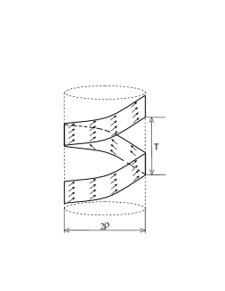
Figure 5: Helical stripe. Arrows represent the projected directions $\{\mathbf{m}\}$ of the tilting molecules on the stripe’s surface.

In the free edge of the helical stripe, we have $v_{b}=v_{t}=0$, $H=-1/2\rho$, $\bar{\phi}=\pi/4-\psi$, $\tau_{\mathbf{m}}=-h/2\rho$, $\kappa_{g}=0$, $\kappa_{n}=-\cos^{2}\psi/\rho$, $\tau_{g}=\sin 2\psi/2\rho$, where $\psi\equiv T/2\pi\rho$ is the pitch angle of the helical stripe. Thus the boundary condition (35) is trivial, and Eqs. (36)–(38) can be transformed into

$$(k_{c}/2)(c_{0}-1/\rho)^{2}+\lambda-h/2\rho=0,$$ (41)

$$k_{c}(c_{0}-1/\rho)+\bar{k}\cos^{2}\psi/\rho-(h/2)\cos 2\psi=0,$$ (42)

$$\gamma\cos^{2}\psi/\rho=0.$$ (43)

If $\gamma\neq 0$, there exists only a trivial solution $\psi=\pi/2$ to the above equations (40)–(43). Thus our theory does not permit genuine helical stripes with free edges with a uniform tilting state.

IV.3 Twisted ribbons

A twisted ribbon with pitch $T$ and width $W$ is shown in Fig. 6, which can be expressed as a a vector $\{u\cos\varphi,u\sin\varphi,\alpha\varphi\}$ with $|u|\leq W/2$, $|\varphi|<\infty$ and $|\alpha|=T/2\pi$. As shown in Appendix G, Eq. (33) is transformed into

$$k_{f}\left(\phi_{uu}+\frac{u\phi_{u}+\phi_{\varphi\varphi}}{u^{2}+\alpha^{2}}\right)+\frac{2h\alpha\sin 2\phi}{u^{2}+\alpha^{2}}=0.$$ (44)

where $\phi$ is the angle between $\mathbf{m}$ and the horizontal.

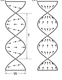
Figure 6: Twisted ribbons: (a) $\mathbf{m}$ is perpendicular to the edges; (b) $\mathbf{m}$ parallels the edges. Arrows represent the projected directions $\{\mathbf{m}\}$ of the tilting molecules on the ribbons’ surface.

If we only consider the uniform tilting state, the above equation requires $\phi=0$ or $\pi/2$. It is easy to see that $\phi=0$ minimizes $-h\int\tau_{\mathbf{m}}dA$ for $\alpha<0$ while $\phi=\pi/2$ minimizes $-h\int\tau_{\mathbf{m}}dA$ for $\alpha>0$ from Eq. (140).Thus we should take $\phi=0$ for $\alpha<0$ and $\phi=\pi/2$ for $\alpha>0$. The former case corresponds to Fig. 6(a) where $\mathbf{m}$ is perpendicular to the edges; the latter corresponds to Fig. 6(b) where $\mathbf{m}$ is parallel to the edges. As shown in Appendix G, both for $\phi=0$ and $\pi/2$, Eq. (34) is transformed into

$$k_{c}c_{0}\alpha^{2}/(u^{2}+\alpha^{2})^{2}=0,$$ (45)

which requires $c_{0}=0$ for non-vanishing $\alpha$. Among the boundary conditions (35)–(38), only Eq. (36) is nontrivial, which gives

$$\lambda(1+x^{2})\alpha^{2}-(h-\gamma x)|\alpha|+\frac{2\bar{k}+k_{f}x^{2}}{2(1+x^{2})}=0,$$ (46)

with $x\equiv W/2|\alpha|$.

Guided by the experimental data Oda99 , we may assume $h$ to be proportional to $R_{d}$, the relative concentration difference of the left- and right-handed enantiomers in the experiment, i.e., $h=h_{0}R_{d}$ with a constant $h_{0}$. In terms of the experimental data, $|\alpha|\rightarrow\infty$ for $R_{d}\rightarrow 0$. Thus Eq. (46) requires $\lambda=0$ and then

$$|\alpha|=(2\bar{k}+k_{f}x^{2})/2(h_{0}R_{d}-\gamma x)(1+x^{2}).$$ (47)

To determine the relation between $x$ and $R_{d}$, we minimize the average energy per area with respect to $|\alpha|$ for given $W$. The average energy per area is calculated as

$$\bar{F}=\frac{(2\bar{k}-k_{f})x+(k_{f}-2h_{0}R_{d}|\alpha|)\sqrt{1+x^{2}}\mathrm{arcsinh}x+2\gamma|\alpha|(1+x^{2})}{\alpha^{2}\sqrt{1+x^{2}}(\mathrm{arcsinh}x+x\sqrt{1+x^{2}})}.$$ (48)

Minimizing it with respect to $|\alpha|$ and using Eq. (47), we obtain

$$x=\beta R_{d}+O(R_{d}^{3}),$$ (49)

with $\beta\equiv 3h_{0}/4\gamma$. This relation reveals that the ratio between the width and pitch of the ribbons is proportional to the relative concentration difference of left- and right-handed enantiomers in the low relative concentration difference region. Eq. (49) fits well with the experimental data with parameter $\beta=0.37$ as shown in Fig. 7.

Figure 7: Relation between $x=W/2|\alpha|$ and $R_{d}$. The solid line is the fitting curve $x=0.37R_{d}$ and the dots are the experimental data in Ref. Oda99 .

V Conclusion and discussion

In this paper, we have focused on a concise free energy from which the Euler-Lagrange equations of CLMs without free edges and Euler-Lagrange equations as well as boundary conditions of CLMs with free edges can be derived analytically. Their implications for extant and future experiments can be summarized as follows.

(i) Our theory predicts the same probability for left- and right-handed spherical vesicles existing in solution. Thus no evident circular dichroism signal should be observed, which is consistent with the experiment Schnur94 .

(ii) The radius of a tubule at uniform tilting state satisfies Eq. (13). It reveals that the radius is independent of molecular chirality, which is consistent with the experiment Spector98 where the tubular radius is insensitive to the proportion of left- and right-handed DC${}_{8,9}PC$ in the tubule. We find that the projected direction of the molecules on the tubular surface departs 45^∘ from the equator of the tubule with the uniform tilting state, which is in good agreement with the experiment Zhaoy05 .

(iii) Tubules with helically modulated tilting state are not admitted by the Euler-Lagrange equation (11) for non-vanishing $h$. The orientational variation of the tilting lipid molecules breaks the force balance along the normal direction of the tubule. Thus a tubule with helically modulated tilting state is not an equilibrium structure within our theoretical framework.

(iv) Helical ripples in tubules are equilibrium structures. The pitch angle of helical ripples is estimated as about 0^∘ and 35^∘ for $k_{f}\simeq k_{c}$, which are close to the experimental values 5^∘ and 28^∘ observed by Fang’s group Zhaoy06 .

(v) Tori with a ratio of generated radii larger than $\sqrt{2}$ are predicted by our theory, Eq. (31), which have not yet been observed in the experiments.

(vi) Helical stripes with free edges at either uniform tilting state or helical modulated tilting state are not possible equilibrium configurations.

(vii) Twisted ribbons satisfy Euler-Lagrange equations (33), (34) and boundary conditions (35)–(38). The ratio between the width and pitch of the ribbons is proportional to the relative concentration difference of left- and right-handed enantiomers in the low relative concentration difference region, which is in good agreement with the experiment Oda99 .

Finally, we have to list a few open problems which should be addressed in the future work.

(i) Within the present theory, we cannot give a simple explanation for the experiments on CLMs of pure cholesterol Chung93 ; Zastavker where helical stripes with pitch angles $11^{\circ}$ and $54^{\circ}$ are usually observed. It has recently been found that the cholesterol helical stripes have good crystal structure Khaykovich07 , which is out of the range of our theory. There might be two possible ramifications based on the present theory: One would be to include anisotropic bending effects ChenCM99 in the free energy density (8); Another one would be to consider a line tension $\gamma$ depending on the angle between the directions of the tilting and the free edges Sarasij02 in the free energy (32).

(ii) We cannot yet interpret the twisted ribbon-to-tubule transition with increasing the relative concentration difference of the left- and right-handed enantiomers reported in the recent experiment by Oda’s group OdaJACS07 . A possible reason is that the parameters except $h$ in our theory are independent of the relative concentration difference odacom . Additionally, the ribbons and tubules observed in this experiment are usually multi-bilayer structures odacom . Then a decoupling effect Seifert96 ; Fournier between neighbor bilayers might occur. An extended theory including these two factors might be required to investigate the mechanism responsible for the transition.

(iii) We have ignored the effect of singular points in CLMs. Although the features of singular points in 2D planar films or achiral nematic spherical, torus vesicles and other manifolds have been fully investigated in previous literature Sarasij02 ; Langer92 ; PetteyPRE99 ; VitelliPRE06 ; Powers07 , it remains a challenge to study the properties of singular points in CLMs rmkspoint .

Appendix A Brief introduction to moving frame method and exterior differential forms

If we take a frame $\{\mathbf{e}_{1},\mathbf{e}_{2},\mathbf{e}_{3}\}$ at any point $\mathbf{r}$ on a surface as shown in Fig. 1, then the infinitesimal tangential vector at $\mathbf{r}$ is expressed as

$$d\mathbf{r}=\omega_{1}\mathbf{e}_{1}+\omega_{2}\mathbf{e}_{2}$$ (50)

and the difference of frame between at points $\mathbf{r}+d\mathbf{r}$ and $\mathbf{r}$ is denoted as

$$d\mathbf{e}_{i}=\omega_{ij}\mathbf{e}_{j},\quad(i=1,2,3),$$ (51)

where $\omega_{1}$, $\omega_{2}$, and $\omega_{ij}=-\omega_{ji},(i,j=1,2,3)$ are 1-forms tzcjpa ; Chernbook . The repeated subscripts in Eq. (51) and the following contents represent the Einstein summation convention. With these 1-forms, the structure equations of a surface can be expressed as tzcjpa ; Chernbook

$$\left\{\begin{array}[]{l}d\omega_{1}=\omega_{12}\wedge\omega_{2},\\ d\omega_{2}=\omega_{21}\wedge\omega_{1},\\ d\omega_{ij}=\omega_{ik}\wedge\omega_{kj}\quad(i,j=1,2,3),\end{array}\right.$$ (52)

and

$$\left(\begin{array}[]{l}\omega_{13}\\ \omega_{23}\end{array}\right)=\left(\begin{array}[]{cc}a&b\\ b&c\end{array}\right)\left(\begin{array}[]{l}\omega_{1}\\ \omega_{2}\end{array}\right),$$ (53)

where the symbol ‘$\wedge$’ expresses the wedge product between differential forms and ‘$d$’ is the exterior differential operator tzcjpa ; Chernbook . The matrix $\left(\begin{array}[]{cc}a&b\\ b&c\end{array}\right)$ is called the curvature matrix which is related to the mean and gaussian curvature by

$$2H=a+c,\quad K=ac-b^{2}.$$ (54)

For a unit vector $\mathbf{m}=\cos\phi\mathbf{e}_{1}+\sin\phi\mathbf{e}_{2}$, the normal curvature along the direction of $\mathbf{m}$ can be expressed as tzcjpa

$$\kappa_{\mathbf{m}}=a\cos^{2}\phi+2b\cos\phi\sin\phi+c\sin^{2}\phi.$$ (55)

The normal curvature along the direction of an arbitrary vector $\mathbf{v}$ can be expressed as

$$\kappa_{\mathbf{v}}=(av_{1}^{2}+2bv_{1}v_{2}+cv_{2}^{2})/\mathbf{v}^{2},$$ (56)

where $v_{1}$ and $v_{2}$ are the components of $\mathbf{v}$ in the directions of $\mathbf{e}_{1}$ and $\mathbf{e}_{2}$.

In our following derivations, several relations between vector forms and differential forms are used frequently. For convenience, we list them below.

$$(\nabla\times\mathbf{m})dA=d(\mathbf{m}\cdot d\mathbf{r}),$$ (57)

$$(\nabla\cdot\mathbf{m})dA=d(\ast\mathbf{m}\cdot d\mathbf{r}),$$ (58)

$$\tau_{\mathbf{m}}dA=\mathbf{m}\cdot d\mathbf{e}_{3}\wedge\mathbf{m}\cdot d\mathbf{r},$$ (59)

$$\kappa_{\mathbf{m}}dA=-\mathbf{m}\cdot d\mathbf{e}_{3}\wedge\ast\mathbf{m}\cdot d\mathbf{r},$$ (60)

$$\nabla\phi\cdot d\mathbf{r}=d\phi,$$ (61)

$$(\nabla^{2}\phi)dA=d\ast d\phi,$$ (62)

$$\mathbf{S}\cdot d\mathbf{r}=-\omega_{12},$$ (63)

$$(\nabla\cdot\mathbf{S})dA=-d\ast\omega_{12},$$ (64)

$$(\nabla\times\mathbf{S})dA=-d\omega_{12}=KdA,$$ (65)

$$\mathbf{v}\cdot d\mathbf{r}=d\phi+\omega_{12},$$ (66)

$$\mathbf{v}^{2}dA=\mathbf{v}\cdot d\mathbf{r}\wedge\ast\mathbf{v}\cdot d\mathbf{r},$$ (67)

$$(\nabla\mathbf{v}\colon\nabla\mathbf{e}_{3})dA=d(\mathbf{v}\cdot d\mathbf{e}_{3}),$$ (68)

where $dA=\omega_{1}\wedge\omega_{2}$ is the area element. $\mathbf{m}$ is a unit vector and $\phi$ is the angle between $\mathbf{m}$ and $\mathbf{e}_{1}$. $\mathbf{S}$ is the spin connection and $\mathbf{v}\equiv\nabla\phi-\mathbf{S}$. $\ast$ is the Hodge star operator tzcjpa ; Westenholzbk which satisfies $\ast\omega_{1}=\omega_{2}$ and $\ast\omega_{2}=-\omega_{1}$.

Using Eqs. (54), (56), (57), (58) and (66), we can prove

$$(\kappa_{\mathbf{v}}-H)\mathbf{v}^{2}=(v_{1}^{2}-v_{2}^{2})(a-c)/2+2bv_{1}v_{2},$$ (69)

and

$$[\nabla\cdot(\mathbf{m}\nabla\times\mathbf{m})+\nabla\times(\mathbf{m}\nabla\cdot\mathbf{m})]dA$$ (70)

$$=d[(v_{2}\cos 2\phi-v_{1}\sin 2\phi)\omega_{1}+(v_{1}\cos 2\phi+v_{2}\sin 2\phi)\omega_{2}],$$

where $v_{1}$ and $v_{2}$ are the components of $\mathbf{v}$ in the directions of $\mathbf{e}_{1}$ and $\mathbf{e}_{2}$.

We suggest the reader refer first to Ref. tzcjpa and some textbook on the calculus with the moving frame method before going on if he is interested in the mathematical details. In writing the following contents we assume that the reader has been familiar with the skill in Ref. tzcjpa and good at calculus with the moving frame method.

Appendix B Derivation of the Euler-Lagrange equations of CLMS without free edges

Here the CLMS without free edges will be derived through the variational method developed in Ref. tzcjpa with the aid of the moving frame method and exterior differential forms, which can highly simplify the calculus of variation.

B.1 Variation respect to $\phi$

Assume $\delta\phi=\Xi$. Through simple calculations, we arrive at

$$\delta\tau_{\mathbf{m}}=2(H-\kappa_{\mathbf{m}})\Xi,$$ (71)

and

$$\delta(\mathbf{v}^{2}dA)=2d\Xi\wedge\ast(d\phi+\omega_{12}).$$ (72)

Combining with the above two equations and using the integral by parts and Stokes’ theorem, we derive

$$\delta F=\int[2h(\kappa_{\mathbf{m}}-H)-k_{f}\nabla^{2}\phi]\Xi dA+k_{f}\oint\Xi\ast\mathbf{v}\cdot d\mathbf{r},$$ (73)

where the second term is the integral along the boundary curve, which vanishes for CLMS without free edges. Since $\Xi$ is an arbitrary function, from $\delta F=0$ we derive Euler-Lagrange equation (10). We have used the assumption $\nabla\cdot\mathbf{S}=0$ when we write Eq. (73). This assumption is indeed satisfied in our discussions on all configurations except ripples in tubules. Thus $\nabla^{2}\phi$ should be replaced with $\nabla^{2}\phi-\nabla\cdot\mathbf{S}$ in Eq. (73) as well as Eq. (10) when this condition is not met.

B.2 Variation respect to the deformation of the surface

In this subsection, let us denote $F_{0}$ as the functional (9) with $h$ and $k_{f}$ vanishing, and define the additional functional

$$F_{ad}=\int\left(\frac{k_{f}}{2}\mathbf{v}^{2}-h\tau_{\mathbf{m}}\right)dA.$$ (74)

Any small deformation of a CLM without free edges can always be achieved from small normal displacement $\Omega_{3}$ at each point $\mathbf{r}$ in the surface. That is, $\delta\mathbf{r}=\Omega_{3}\mathbf{e}_{3}$. The frame is also changed because of the deformation of the surface, which is denoted as

$$\delta\mathbf{e}_{i}=\Omega_{ij}\mathbf{e}_{j},\quad(i=1,2,3),$$ (75)

where $\Omega_{ij}=-\Omega_{ji},(i,j=1,2,3)$ corresponds to the rotation of the frame due to the deformation of the surface.

$\delta F_{0}$ was first dealt with in Ref. oy90 which gives

$$\delta F_{0} = \int(2k_{c}\nabla^{2}H-2\lambda H+P)\Omega_{3}dA$$ (76)

$$+ \int k_{c}(2H+c_{0})(2H^{2}-c_{0}H-2K)\Omega_{3}dA.$$

Following Ref. tzcjpa , and considering Eqs. (59), (66) and (67), through somewhat involved calculations, we can derive

$$\delta(\tau_{\mathbf{m}}dA)=2\Omega_{12}(H-\kappa_{\mathbf{m}})dA+\nabla\cdot\mathbf{m}d\Omega_{3}\wedge\mathbf{m}\cdot d\mathbf{r}$$

$$\hskip 39.83368pt+\mathbf{m}\cdot d\mathbf{r}\wedge d(d\Omega_{3}\wedge\ast\mathbf{m}\cdot d\mathbf{r}/dA),$$ (77)

$$\delta(\mathbf{v}^{2}dA)=2d\Omega_{12}\wedge\ast(d\phi+\omega_{12})$$

$$\hskip 39.83368pt+2d\Omega_{3}\wedge\mathbf{v}\cdot{d}\mathbf{e}_{3}+2(\kappa_{\mathbf{v}}-H)\mathbf{v}^{2}\Omega_{3}dA.$$ (78)

Combining with the above two equations and using the integral by parts and Stokes’ theorem, we derive

$$\delta F_{ad}=\int h[\nabla\cdot(\mathbf{m}\nabla\times\mathbf{m})+\nabla\times(\mathbf{m}\nabla\cdot\mathbf{m})]\Omega_{3}dA$$

$$\hskip 24.18501pt+\int k_{f}[(\kappa_{\mathbf{v}}-H)\mathbf{v}^{2}-\nabla\mathbf{v}\colon\nabla\mathbf{e}_{3}]\Omega_{3}dA,$$ (79)

Then the Euler-Lagrange equation (11) follows from $\delta F=\delta F_{0}+\delta F_{ad}=0$ because $\Omega_{3}$ is an arbitrary function.

Appendix C Derivation of the Euler-Lagrange equations and boundary conditions of CLMS with free edges

A CLM with an free edge can be described as a surface with an boundary curve shown in Fig. 1B.

C.1 Variation respect to $\phi$

Let $\delta\phi=\Xi$, we still have Eq. (73) whose second term is transformed into

$$-k_{f}\oint v_{b}\Xi ds$$ (80)

with $v_{b}=\mathbf{v}\cdot\mathbf{b}$. Thus from $\delta F=0$ we can derive the Euler-Lagrange equation (33) and boundary condition (35).

C.2 Variation respect to the deformation of the surface

Because one can select an arbitrary frame $\{\mathbf{r};\mathbf{e}_{1},\mathbf{e}_{2},\mathbf{e}_{3}\}$, here we take it such that $\mathbf{e}_{1}$ and $\mathbf{e}_{2}$ align with $\mathbf{t}$ and $\mathbf{b}$ in the boundary curve. Then any small deformation of a CLM with an free edge can always be expressed as the linear superposition of small normal displacement $\Omega_{3}$ and tangent displacement $\Omega_{2}$ along $\mathbf{e}_{2}$ at each point $\mathbf{r}$ in the surface.

First, we consider the in-plane deformation mode $\delta\mathbf{r}=\Omega_{2}\mathbf{e}_{2}$. The change of the frame is still denoted as Eq. (75). In terms of Ref. tzcpre , we have $\delta\oint ds=-\oint\kappa_{g}\Omega_{2}ds$ where $\kappa_{g}$ is the geodesic curvature of the boundary curve. Additionally, we can derive

$$\delta\int GdA=-\oint G\Omega_{2}ds.$$ (81)

Although the derivation of the above equation is somewhat involved, its physical meaning is quite clear. Under the displacement $\Omega_{2}$ along $\mathbf{e}_{2}$, $G$ is similar to the surface tension and the area element near the boundary decreases by $\Omega_{2}ds$. Thus the variation of $\int GdA$ gives Eq. (81) and then we obtain the boundary condition (36) from $\delta F=0$.

Second, we consider the out-of-plane deformation mode $\delta\mathbf{r}=\Omega_{3}\mathbf{e}_{3}$. Let us denote $F_{0}$ as the functional (32) with $h$ and $k_{f}$ vanishing, and define the additional functional as Eq. (74). $\delta F_{0}$ is fully discussed in Ref. tzcpre as

$$\delta F_{0}=\int[k_{c}(2H+c_{0})(2H^{2}-c_{0}H-2K)-2\lambda H]\Omega_{3}dA$$

$$+\int 2k_{c}(\nabla^{2}H)\Omega_{3}dA-\oint[k_{c}(2H+c_{0})-\bar{k}\kappa_{n}]\Omega_{23}ds$$

$$-\oint[-2k_{c}\partial H/\partial\mathbf{b}+\gamma\kappa_{n}-\bar{k}\dot{\tau}_{g}]\Omega_{3}ds.$$ (82)

Here the only difference is that the sign of $\bar{k}$ adopted in the present paper is opposite to that in Ref. tzcpre . Similar to the derivation of Eq. (79) from Eqs. (77) and (78) by using the integral by parts and Stokes’ theorem, we have

$$\delta F_{ad} = \int h[\nabla\cdot(\mathbf{m}\nabla\times\mathbf{m})+\nabla\times(\mathbf{m}\nabla\cdot\mathbf{m})]\Omega_{3}dA$$ (83)

$$+ \int k_{f}[(\kappa_{\mathbf{v}}-H)\mathbf{v}^{2}-\nabla\mathbf{v}\colon\nabla\mathbf{e}_{3}]\Omega_{3}dA$$

$$+ \oint[h(v_{t}+\dot{\bar{\phi}})\sin 2\bar{\phi}-k_{f}\kappa_{n}v_{t}]\Omega_{3}ds$$

$$+ \oint(h/2)\sin 2\bar{\phi}\Omega_{23}ds,$$

where $v_{t}=\mathbf{v}\cdot\mathbf{t}$. In the above equations (82) and (83), $\Omega_{3}$ represents the arbitrary small displacement of point on the surface along $\mathbf{e}_{3}$ and $\Omega_{23}$ is the arbitrary small rotation of $\mathbf{e}_{3}$ around $\mathbf{t}$ at the edge. Thus $\delta F=0$ will give the Euler-Lagrange equation (34) and boundary conditions (37) and (38).

Appendix D Derivation of equations (14) and (15) for tubules with nonuniform tilting state in Section III.4

For a cylindrical surface, take a frame such that $\mathbf{e}_{1}$, $\mathbf{e}_{2}$ and $\mathbf{e}_{3}$ are along the circumferential, axial and radial directions, respectively. Then we have

$$\omega_{1}=ds,\omega_{2}=dz$$ (84)

$$a=-1/\rho,b=c=0.$$ (85)

Thus

$$2H=a+c=-1/\rho,K=ac-b^{2}=0.$$ (86)

Because $dds=0$ and $ddz=0$, using the structure equation (52), we have $\omega_{12}=0$. Considering Eq. (63), we obtain the spin connection

$$\mathbf{S}=0,$$ (87)

and then

$$\mathbf{v}=\nabla\phi=\phi_{s}\mathbf{e}_{1}+\phi_{z}\mathbf{e}_{2}.$$ (88)

From Eqs. (55) and (62), we have

$$\kappa_{\mathbf{m}}=-\cos^{2}\phi/\rho,$$ (89)

$$\nabla^{2}\phi=\phi_{ss}+\phi_{zz}.$$ (90)

Substituting the above two equations and Eq. (86) into the Euler-Lagrange equation (10), we can derive Eq. (14) in Sec. III.4.

Additionally, using Eqs. (51), (53) and (88), we derive

$$\mathbf{v}\cdot d\mathbf{e}_{3}=(\phi_{s}/\rho)ds.$$ (91)

From Eq. (68) we can derive

$$\nabla\mathbf{v}\colon\nabla\mathbf{e}_{3}=-\phi_{sz}/\rho.$$ (92)

In this derivation, one should note that $dA=ds\wedge dz=-dz\wedge ds$. From Eqs. (69), (70), (85) and (88), we can obtain

$$(\kappa_{\mathbf{v}}-H)\mathbf{v}^{2}=(\phi_{z}^{2}-\phi_{s}^{2})/2\rho,$$ (93)

and

$$\nabla\cdot(\mathbf{m}\nabla\times\mathbf{m})+\nabla\times(\mathbf{m}\nabla\cdot\mathbf{m})$$ (94)

$$=2\sin 2\phi(\phi_{z}^{2}-\phi_{s}^{2}+\phi_{sz})+\cos 2\phi(\phi_{ss}-\phi_{zz}+4\phi_{z}\phi_{s}).$$

Substituting Eqs. (86) and (92)–(94) into the Euler-Lagrange equation (11), we can obtain Eq. (15) in Sec. III.4.

Appendix E Derivation of equations (20) and (21) for helical ripples in Section III.5

For the surface expressed as vector form

$$\mathbf{r}=\{\rho(1+y)\cos(s/\rho),\rho(1+y)\sin(s/\rho),z\}$$ (95)

with $|y|\ll 1$, the first and second fundamental forms of the surface can be calculated as

$$I=(1+2y)ds^{2}+dz^{2},$$ (96)

$$II=-\frac{1}{\rho}(1+y-\rho^{2}y_{ss})ds^{2}+2\rho y_{sz}dsdz+\rho y_{zz}dz^{2}$$ (97)

up to the order of $O(y)$, respectively. The same order is kept in the following expressions in this section. In terms of the correspondence relations $I=\omega_{1}^{2}+\omega_{2}^{2}$ and $II=a\omega_{1}^{2}+2b\omega_{1}\omega_{2}+\omega_{2}^{2}$, we have

$$\omega_{1}=(1+y)ds,\omega_{2}=dz,$$ (98)

$$a=-(1-y-\rho^{2}y_{ss})/{\rho},b=\rho y_{sz},c=\rho y_{zz},$$ (99)

$$2H=-(1-y-\rho^{2}y_{ss}-\rho^{2}y_{zz})/{\rho},K=-y_{zz}.$$ (100)

$2H$ is a function of $s$ and $z$, using $\nabla^{2}(2H)dA=d\ast d(2H)$, we can derive

$$\nabla^{2}(2H)=(y_{ss}+y_{zz}+\rho^{2}y_{ssss}+2\rho^{2}y_{zzss}+\rho^{2}y_{zzzz})/\rho$$ (101)

Because $d\omega_{1}=y_{z}dz\wedge ds$ and $d\omega_{2}=ddz=0$, using the structure equation (52), we have $\omega_{12}=-y_{z}\omega_{1}$. Considering Eqs. (63) and (64), we have

$$\mathbf{S}=y_{z}\mathbf{e}_{1},\nabla\cdot\mathbf{S}=y_{zs}.$$ (102)

Using Eqs. (61) and (62), we obtain

$$\nabla\phi=\phi_{s}(1-y)\mathbf{e}_{1}+\phi_{z}\mathbf{e}_{2}$$ (103)

$$\nabla^{2}\phi=\phi_{ss}+\phi_{zz}+\phi_{z}y_{z}-\phi_{s}y_{s}-2y\phi_{ss}.$$ (104)

and then

$$\mathbf{v}=\nabla\phi-\mathbf{S}=[\phi_{s}(1-y)-y_{z}]\mathbf{e}_{1}+\phi_{z}\mathbf{e}_{2}.$$ (105)

From Eqs. (51), (53), (68), (69), and (105), we can derive

$$\nabla\mathbf{v}\colon\nabla\mathbf{e}_{3}=-\phi_{sz}/\rho+(y_{z}\phi_{s}+2y\phi_{sz}+y_{zz})/\rho,$$ (106)

$$(\kappa_{\mathbf{v}}-H)\mathbf{v}^{2}=(\phi_{z}^{2}-\phi_{s}^{2})/{2\rho}+\phi_{s}(y\phi_{s}+y_{z})/{\rho}$$

$$+2\rho y_{sz}\phi_{s}\phi_{z}+(y+\rho^{2}y_{ss}-\rho^{2}y_{zz})(\phi_{s}^{2}-\phi_{z}^{2})/2\rho.$$ (107)

Since we only consider the case of $\bar{h}\ll 1$, up to the order $O(\bar{h})$, we obtain

$$\bar{h}(\kappa_{\mathbf{m}}-H)=-(\bar{h}/2\rho)\cos 2\phi,$$ (108)

$$\bar{h}[\nabla\cdot(\mathbf{m}\nabla\times\mathbf{m})+\nabla\times(\mathbf{m}\nabla\cdot\mathbf{m})]$$ (109)

$$=\bar{h}[2(\phi_{z}^{2}-\phi_{s}^{2}+\phi_{sz})\sin 2\phi+(\phi_{ss}-\phi_{zz}+4\phi_{z}\phi_{s})\cos 2\phi]$$

by using Eqs. (55) and (94).

Substituting the above equations (100)–(109) into the Euler-Lagrange equations (10) and (11), we can derive the basic equations (20) and (21) under the assumption $c_{0}=0$, $\lambda=0$, $k_{f}\simeq k_{c}$ in Sec. III.5.

Appendix F Derivation of equations (29) and (30) for tori in Section III.6

A torus can be expressed as a vector form

$$\mathbf{r}=\{(r+\rho\cos\varphi)\cos\theta,(r+\rho\cos\varphi)\sin\theta,\rho\sin\varphi\}$$ (110)

with $r>\rho$. A frame $\{\mathbf{e}_{1},\mathbf{e}_{2},\mathbf{e}_{3}\}$ is taken as

$$\left\{\begin{array}[]{l}\mathbf{e}_{1}=\{-\sin\theta,\cos\theta,0\},\\ \mathbf{e}_{2}=\{-\sin\varphi\cos\theta,-\sin\varphi\sin\theta,\cos\varphi\},\\ \mathbf{e}_{3}=\{\cos\theta\cos\varphi,\sin\theta\cos\varphi,\sin\varphi\}.\end{array}\right.$$ (111)

By using Eqs. (50), (110) and (111), we can derive

$$\omega_{1}=(r+\rho\cos\varphi)d\theta,\omega_{2}=\rho d\varphi.$$ (112)

From Eq. (51) and (111), we obtain

$$\omega_{12}=[{\sin\varphi}/{(r+\rho\cos\varphi)}]\omega_{1},$$ (113)

$$\omega_{13}=-[{\cos\varphi}/{(r+\rho\cos\varphi)}]\omega_{1},$$ (114)

$$\omega_{23}=-(1/\rho)\omega_{2}.$$ (115)

Considering Eqs. (63), (64) and (113), we have

$$\mathbf{S}=-[{\sin\varphi}/{(r+\rho\cos\varphi)}]\mathbf{e}_{1},$$ (116)

$$\nabla\cdot\mathbf{S}=0.$$ (117)

Additionally, (53), (114) and (115) give

$$a=-{\cos\varphi}/{(r+\rho\cos\varphi)},b=0,c=-1/\rho.$$ (118)

Thus by considering Eqs. (3), (54), (55), and (62), we obtain

$$2H=-\frac{r+2\rho\cos\varphi}{\rho(r+\rho\cos\varphi)},K=\frac{\cos\varphi}{\rho(r+\rho\cos\varphi)},$$ (119)

$$\kappa_{\mathbf{m}}=-\frac{\cos^{2}\phi\cos\varphi}{r+\rho\cos\varphi}-\frac{\sin^{2}\phi}{\rho},$$ (120)

$$\tau_{\mathbf{m}}=-\frac{r\sin 2\phi}{2\rho(r+\rho\cos\varphi)},$$ (121)

$$\nabla^{2}\phi=\frac{\phi_{\theta\theta}}{(r+\rho\cos\varphi)^{2}}+\frac{\phi_{\varphi\varphi}}{\rho^{2}}-\frac{\sin\varphi\phi_{\varphi}}{\rho(r+\rho\cos\varphi)}.$$ (122)

Substituting the above four equations into Eq. (10), we can derive Eq. (29) in Sec. III.6.

If $\phi=-\pi/4$, then $\nabla\phi=0$, and

$$\mathbf{v}\equiv\nabla\phi-\mathbf{S}=[{\sin\varphi}/{(r+\rho\cos\varphi)}]\mathbf{e}_{1},$$ (123)

$$\mathbf{v}\cdot d\mathbf{e}_{3}=v_{1}\omega_{31}=[\sin 2\varphi/2(r+\rho\cos\varphi)]d\theta,$$ (124)

where $v_{1}$ is the component of $\mathbf{v}$ in the direction of $\mathbf{e}_{1}$. Thus from Eq. (68) we can derive

$$\nabla\mathbf{v}\colon\nabla\mathbf{e}_{3}=-(r\cos 2\varphi+\rho\cos^{3}\varphi)/\rho(r+\rho\cos\varphi)^{3}.$$ (125)

Using Eqs. (69), (70), (118) and (123), we can obtain

$$(\kappa_{\mathbf{v}}-H)\mathbf{v}^{2}={r\sin^{2}\varphi}/{2\rho(r+\rho\cos\varphi)^{3}},$$ (126)

and

$$\nabla\cdot(\mathbf{m}\nabla\times\mathbf{m})+\nabla\times(\mathbf{m}\nabla\cdot\mathbf{m})=-\cos\varphi/\rho(r+\rho\cos\varphi).$$ (127)

Additionally, from $\nabla^{2}(2H)dA=d\ast d(2H)$, we have

$$\nabla^{2}(2H)=r(r\cos\varphi+\rho)/\rho^{2}(r+\rho\cos\varphi)^{3}.$$ (128)

Substituting the above equations (119) and (125)–(128) into Eq. (11), we can derive Eq. (30) in Sec. III.6.

Appendix G Derivation of equations (44)–(46), and (48) for twisted ribbons in Section IV.3

A twisted ribbon can be expressed as a vector form

$$\mathbf{r}=\{u\cos\varphi,u\sin\varphi,\alpha\varphi\}$$ (129)

A frame $\{\mathbf{e}_{1},\mathbf{e}_{2},\mathbf{e}_{3}\}$ is taken as

$$\left\{\begin{array}[]{l}\mathbf{e}_{1}=\{\cos\varphi,\sin\varphi,0\},\\ \mathbf{e}_{2}=\{-u\sin\varphi,u\cos\varphi,\alpha\}/\sqrt{u^{2}+\alpha^{2}},\\ \mathbf{e}_{3}=\{\alpha\sin\varphi,-\alpha\cos\varphi,u\}/\sqrt{u^{2}+\alpha^{2}}.\end{array}\right.$$ (130)

By using Eqs. (50), (129) and (130), we can derive

$$\omega_{1}=du,\omega_{2}=\sqrt{u^{2}+\alpha^{2}}d\varphi.$$ (131)

From Eq. (51) and (130), we obtain

$$\omega_{12} = [u/(u^{2}+\alpha^{2})]\omega_{2},$$ (132)

$$\omega_{13} = -[\alpha/(u^{2}+\alpha^{2})]\omega_{2},$$ (133)

$$\omega_{23} = -[\alpha/(u^{2}+\alpha^{2})]\omega_{1}.$$ (134)

Considering Eqs. (63), (64) and (132), we have

$$\mathbf{S}=-[u/(u^{2}+\alpha^{2})]\mathbf{e}_{2},$$ (135)

$$\nabla\cdot\mathbf{S}=0.$$ (136)

Additionally, (53), (133) and (134) give

$$a=c=0,b=-\alpha/(u^{2}+\alpha^{2}).$$ (137)

Thus by considering Eqs. (3), (54), (55), and (62), we obtain

$$H=0,K=-\alpha^{2}/(u^{2}+\alpha^{2})^{2},$$ (138)

$$\kappa_{\mathbf{m}}=-\alpha\sin 2\phi/(u^{2}+\alpha^{2}),$$ (139)

$$\tau_{\mathbf{m}}=-\alpha\cos 2\phi/(u^{2}+\alpha^{2}),$$ (140)

$$\nabla^{2}\phi=\phi_{uu}+(u\phi_{u}+\phi_{\varphi\varphi})/(u^{2}+\alpha^{2}).$$ (141)

Substituting the above four equations into Eq. (33), we can derive Eq. (44) in Sec. IV.3.

If $\phi=0$ or $\pi/2$, then $\nabla\phi=0$, and

$$\mathbf{v}\equiv\nabla\phi-\mathbf{S}=[u/(u^{2}+\alpha^{2})]\mathbf{e}_{2},$$ (142)

$$\mathbf{v}\cdot d\mathbf{e}_{3}=v_{2}\omega_{32}=[u\alpha/(u^{2}+\alpha^{2})^{2}]du,$$ (143)

where $v_{2}$ is the component of $\mathbf{v}$ in the direction of $\mathbf{e}_{2}$. Thus from Eq. (68) we can derive

$$\nabla\mathbf{v}\colon\nabla\mathbf{e}_{3}=0.$$ (144)

Considering $\sin 2\phi=0$ and $\cos 2\phi=\pm 1$, from Eqs. (69), (70), (137) and (142), we can obtain

$$(\kappa_{\mathbf{v}}-H)\mathbf{v}^{2}=0,$$ (145)

$$\nabla\cdot(\mathbf{m}\nabla\times\mathbf{m})+\nabla\times(\mathbf{m}\nabla\cdot\mathbf{m})=0.$$ (146)

Substituting the above equations (138) and (144)–(146) into Eq. (34), we can derive Eq. (45) in Sec. IV.3.

Now let us turn to the boundary conditions. If $\phi=0$ for $\alpha<0$, we have $\bar{\phi}=\pm\frac{\pi}{2}$. At the boundary, $\mathbf{t}\|\mathbf{e}_{2}$ and $u=u_{0}\equiv W/2$, so

$$v_{t}=u_{0}/(u_{0}^{2}+\alpha^{2}),v_{b}=0.$$ (147)

From Eqs. (138)–(140), we can obtain

$$K=-\alpha^{2}/(u_{0}^{2}+\alpha^{2})^{2},$$ (148)

$$\kappa_{\mathbf{m}}=0,\tau_{\mathbf{m}}=-\alpha/(u_{0}^{2}+\alpha^{2}).$$ (149)

Additionally, we have

$$\kappa_{n}=a\cos^{2}(\pi/2)+b\sin\pi+c^{2}\sin(\pi/2)=0,$$ (150)

$$\kappa_{g}=\omega_{12}/\omega_{2}=u_{0}/(u_{0}^{2}+\alpha^{2}),$$ (151)

$$\tau_{g}=b\cos\pi+(c-a)(\sin\pi)/2=\alpha/(u_{0}^{2}+\alpha^{2}),$$ (152)

in terms of the definition of normal curvature, geodesic curvature and geodesic torsion. From the above equations (147)–(152), we find that among the boundary conditions (35)–(38), only Eq. (36) is nontrivial, which gives Eq. (46). Similarly, we obtain the same equation as (46) when $\phi=\pi/2$ for $\alpha>0$.

The average energy per area (48) can be obtained from $F/A$, where $A$ is the area of the twisted ribbon and $F$ is the free energy (32). The calculation is straightforward with $c_{0}=0$, Eqs. (138), (140), (142), and

$$dA=\sqrt{u^{2}+\alpha^{2}}dud\varphi,$$ (153)

$$ds=\sqrt{u_{0}^{2}+\alpha^{2}}d\varphi.$$ (154)

References

- (1) J. M. Schnur, Science 282, 1669 (1993).
- (2) J. M. Schnur, B. R. Ratna, J. V. Selinger, A. Singh, G. Jyothi, and K. R. K. Easwaran, Science 264, 945 (1994).
- (3) M. S. Spector, J. V. Selinger, A. Singh, J. M. Rodriguez, R. R. Price, and J. M. Schnur, Langmuir 14, 3493 (1998).
- (4) Y. Zhao, N. Mahajan, R. Lu, and J. Fang, Proc. Natl. Acad. Sci. USA 102, 7438 (2005).
- (5) N. Mahajan, Y. Zhao, T. Du, and J. Fang, Langmuir 22, 1973 (2006).
- (6) M.S. Spector, A. Singh, P. B. Messersmith, and J. M. Schnur, Nano Lett. 1, 375 (2001).
- (7) D. S. Chung, G. B. Benedek, F. M. Konikoff, and J. M. Donovan, Proc. Natl. Acad. Sci. USA 90, 11341 (1993)
- (8) Y. V. Zastavker, N. Asherie, A. Lomakin, J. Pande, J. M. Donovan, J. M. Schnur, and G. B. Benedek, Proc. Natl. Acad. Sci. USA 96, 7883 (1999).
- (9) R. Oda, I. Huc, M. Schmutz, S. J. Candau, F. C. MacKintosh, Nature (London) 399, 566 (1999).
- (10) D. Berthier, T. Buffeteau, J. Léger, R. Oda, and I. Huc, J. Am. Chem. Soc. 124, 13486 (2002).
- (11) W. Helfrich and J. Prost, Phys. Rev. A 38, 3065 (1988).
- (12) O. Y. Zhongcan and L. Jixing, Phys. Rev. Lett. 65, 1679 (1990); Phys. Rev. A 43, 6826 (1991).
- (13) P. Nelson and T. Powers, Phys. Rev. Lett. 69, 3409 (1992).
- (14) J. V. Selinger and J. M. Schnur, Phys. Rev. Lett. 71, 4091 (1993).
- (15) J. V. Selinger, F. C. MacKintosh, and J. M. Schnur, Phys. Rev. E 53, 3804 (1996).
- (16) J. V. Selinger, M. S. Spector, and J. M. Schnur, J. Phys. Chem. B 105, 7157 (2001).
- (17) S. Komura and O. Zhong-can, Phys. Rev. Lett. 81, 473 (1998).
- (18) Z. Hu and V. C. Lo, Int. J. Mod. Phys. B 19, 2999 (2005).
- (19) Z. C. Tu and Z. C. Ou-Yang, J. Phys. A 37, 11407 (2004).
- (20) W. Helfrich, Z. Naturforsch. 28C, 693 (1973).
- (21) F. C. MacKintosh and T. C. Lubensky, Phys. Rev. Lett. 67, 1169 (1991); T. C. Lubensky and J. Prost, J. Phys. (France) 2, 371 (1992).
- (22) D. R. Nelson and L. Peliti, J. Phys. France 48, 1085 (1987).
- (23) O. Y. Zhongcan and W. Helfrich Phys. Rev. Lett. 59, 2486, (1987); Phys. Rev. A 39, 5280 (1989).
- (24) R. Lipowsky, Nature (London) 349, 475 (1991).
- (25) U. Seifert, Adv. Phys. 46, 13 (1997).
- (26) Z. C. Ou-Yang, J. X. Liu and Y. Z. Xie, Geometric Methods in the Elastic Theory of Membranes in Liquid Crystal Phases (World Scientific, Singapore, 1999).
- (27) Q. Du, C. Liu and X. Wang, J. Comput. Phys. 212, 757 (2006).
- (28) Y. M. Lvov, R. R. Price, J. V. Selinger, A. Singh, M. S. Spector, and J. M. Schnur, Langmuir 16, 5932 (2000).
- (29) Z. C. Ou-Yang, Phys. Rev. A 41, 4517 (1990).
- (30) U. Seifert, Phys. Rev. Lett. 66, 2404 (1991).
- (31) M. Mutz and D. Bensimon, Phys. Rev. A 43, 4525 (1991).
- (32) A. S. Rudolph, B. R. Ratna, and B. Kahn, Nature (London) 352, 52 (1991).
- (33) Z. Lin, R. M. Hill, H. T. Davis, L. E. Scriven, and Y. Talmon, Langmuir 10, 1008 (1994).
- (34) R. Capovilla, J. Guven, and J. A. Santiago, Phys. Rev. E 66, 021607 (2002).
- (35) Z. C. Tu and Z. C. Ou-Yang, Phys. Rev. E 68, 061915 (2003).
- (36) T. Umeda, Y. Suezaki, K. Takiguchi, and H. Hotani, Phys. Rev. E 71, 011913 (2005).
- (37) X. Wang and Q. Du, e-print arXiv: physics/0605095.
- (38) B. Khaykovich, C. Hossain, J. J. McManus, A. Lomakin, D. E. Moncton, and G. B. Benedek, Proc. Natl. Acad. Sci. USA 104, 9656 (2007).
- (39) C.-M. Chen, Phys. Rev. E 59, 6192 (1999).
- (40) R. C. Sarasij and M. Rao, Phys. Rev. Lett. 88, 088101 (2002); e-print arXiv: cond-mat/0703182.
- (41) A. Brizard, C. Aimé, T. Labrot, I. Huc, D. Berthier, F. Artzner, B. Desbat, and R. Oda, J. Am. Chem. Soc. 129, 3754 (2007).
- (42) R. Oda, private communication.
- (43) U. Seifert, J. Shillcock, and P. Nelson, Phys. Rev. Lett. 77, 5237 (1996).
- (44) J. B. Fournier, Eur. Phys. J. B 11, 261 (1999).
- (45) S. A. Langer, R. E. Goldstein, and D. P. Jackson, Phys. Rev. A 46, 4894 (1992).
- (46) D. Pettey and T. C. Lubensky, Phys. Rev. E 59, 1834 (1999).
- (47) V Vitelli and D. R. Nelson, Phys. Rev. E 74, 021711 (2006).
- (48) H. Jiang, G. Huber, R. A. Pelcovits, and T. R. Powers, e-print arXiv: 0707.4004.
- (49) The property of singular points on spherical CLMs is still same as that on achiral spherical vesicles discussed in VitelliPRE06 . The difference will be evident in non-spherical CLMs.
- (50) S. S. Chern and W. H. Chern, Lecture on Differential Geometry (Beijing University Press, Beijing, 1983).
- (51) C. V. Westenholz, Differential Forms in Mathematical Physics (North-Holland, Amsterdam, 1981).