Variational QMC study of a Hydrogen atom in jellium with comparison to LSDA and LSDA-SIC solutions

Abstract

A Hydrogen atom immersed in a finite jellium sphere is solved using variational quantum Monte Carlo (VQMC). The same system is also solved using density functional theory (DFT), in both the local spin density (LSDA) and self-interaction correction (SIC) approximations. The immersion energies calculated using these methods, as functions of the background density of the jellium, are found to lie within $1eV$ of each other with minima in approximately the same positions. The DFT results show overbinding relative to the VQMC result. The immersion energies also suggest an improved performance of the SIC over the LSDA relative to the VQMC results. The atom-induced density is also calculated and shows a difference between the methods, with a more extended Friedel oscillation in the case of the VQMC result.

I Introduction

The model system of an atom embedded in infinite jellium is of interest because it can be used to describe the bonding of an atom within a solid. The idea is that the atom is embedded in a homogeneous electron gas which is regarded as the sum of the density tails from all other atoms in the solid spatially averaged over the unit cell of the atom in question. The immersion energy of the atom (the total energy of the atom in jellium minus the energies of the separate atom and jellium) can then be regarded as a first order approximation to the cohesive energy per atom of the solid. In fact, within the framework of the effective medium theory (EMT),[1, 2] one includes an additional term in this cohesive energy which describes the electrostatic attraction between the density tails within the unit cell and the Hartree potential set up by the atom. This allows one to calculate cohesive properties of solids across the periodic table and indeed one finds that the Wigner Seitz radii, bulk moduli and cohesive energies follow the same trends as the experimental values.

In this paper the atom in jellium system is solved using the variational quantum Monte Carlo (VQMC) method [3, 4] and the local spin density (LSDA) [5, 6, 7, 8, 9] and self-interaction correction (SIC) [10] approximations of density functional theory (DFT). The particular system used is a Hydrogen atom immersed in jellium. In order to solve this system using VQMC, the system must be of finite size and therefore we approximate the atom in infinite jellium with an atom in a finite jellium sphere centered on the atom. The quantities to be calculated include the total energies of both the Hydrogen in jellium and the jellium sphere by itself, the immersion energy and the atom-induced density (the density of the Hydrogen atom in jellium minus the density of the jellium). These quantities are to be calculated as a function of the positive background density of the jellium, $n_{0}$, for a jellium sphere with a fixed number of electrons.

VQMC calculations have already been attempted on the system of a Hydrogen atom in jellium by Sugiyama et al. [11] These calculations however resulted in immersion energies which differed significantly from the LDA results. Atom-induced densities calculated by Sugiyama et al. were also found to differ significantly between these methods. Our results are based upon a careful study of size effects and show a much closer agreement between LSDA and QMC.

The system of a jellium sphere with no embedded atom has been solved using QMC (in both the variational and diffusion variants) by Sottile et al. [12] Jellium spheres with up to 106 electrons were reported and good agreement was found between the LSDA and the diffusion QMC (DQMC) results.

Work on using a Hydrogen atom in a finite jellium sphere has also been reported [13] within the LSDA. It was shown that by controlling the size of the jellium sphere, a good approximation to Hydrogen in infinite jellium can be obtained.

SIC calculations have already been reported for the atom in infinite jellium system.[14] The EMT was applied, and for atoms up to and including the $2p$ elements the SIC cohesive energy was found to be higher than that of the LSDA. The interpretation placed on this was that the SIC was correcting for the overbinding present in the LSDA. Here we compare SIC with both LSDA and VQMC.

In the following section we first investigate the LSDA solution of a Hydrogen atom in a finite jellium sphere. We examine the effect of changing the jellium sphere size and establish choices of sphere which yield good approximations to the infinite jellium solution. We then consider in Sections III and IV the VQMC and SIC methods for the same finite sphere system. Section V presents a comparison of our VQMC results with those of the LSDA and SIC.

II LSDA solution

II.1 Minimizing the energy functional

We first solve the spin-polarized Kohn-Sham (KS) equations within the LSDA for an external potential set up by a Hydrogen ion and a sphere of positive charge centered on the ion with charge density $n_{0}$ and radius $R_{jell}$. The system is overall charge neutral.

We spherically symmetrize the spin densities, $n^{\sigma}({\bf r})$, after each iteration of the self-consistency cycle before recalculating the KS potentials. The KS potential will therefore also be spherically symmetric and so the KS equations reduce to the radial Schrödinger equations. The self-consistent solutions to these equations minimize the LSDA energy functional

$$E[n^{\uparrow},n^{\downarrow}]=\sum_{n,l,m,\sigma}\int{\psi_{nlm}^{\sigma*}}({\bf r})(-\frac{1}{2}\nabla^{2}){\psi_{nlm}^{\sigma}}({\bf r})d{\bf r}+$$

$$\frac{1}{2}\int\int{n(r)n(r^{\prime})\over{|{\bf r}-{\bf r}^{\prime}|}}d{\bf r}d{\bf r}^{\prime}+\int v_{ext}(r)n(r)d{\bf r}+$$

$$E_{xc}[n^{\uparrow},n^{\downarrow}]+Z\int_{r=0}^{r=R_{jell}}{n_{0}\over{r}}d{\bf r}+\frac{3}{5}{N^{5/3}\over{r_{s}}}$$

where $\psi_{nlm}^{\sigma}({\bf r})$ are the self-consistent KS orbitals, $n^{\sigma}(r)$ are the spherically symmetrized spin densities, $n(r)=\sum_{\sigma}n^{\sigma}(r)$ is the total electron density and $v_{ext}(r)$ is the external potential

$$v_{ext}(r)=-{1\over r}-\int_{r^{\prime}=0}^{R_{jell}}{n_{0}\over{|{\bf r}-{\bf r}^{\prime}|}}d{\bf r}^{\prime}$$

The final two terms in the energy functional include the Coulomb repulsion between the ion and the positive background and the self-Coulomb repulsion of the positive background. The electron density parameter, $r_{s}$ is defined by $\frac{4}{3}\pi r_{s}^{3}n_{0}=1$ and $N=\frac{4}{3}\pi R_{jell}^{3}n_{0}$ is the number of electrons in the jellium sphere.

The kinetic energy can be calculated either by numerically evaluating the radial derivatives of the orbitals, or alternatively by rearranging the KS equations and substituting in for the Laplacian. In our calculations both methods are used and are found to give the same results.

The energy functional is also used to calculate the energy of the separate jellium sphere and Hydrogen atom. The immersion energy is then obtained by subtracting these quantities from the Hydrogen atom in jellium energy.

II.2 Jellium sphere sizes

The number of electrons in the sphere is chosen by studying, within the LSDA, the immersion energy of a Hydrogen atom in a jellium sphere of fixed $n_{0}$ as a function of the number of electrons in the sphere. Figure 1 illustrates the dependence of the immersion energy on the size of the jellium sphere for a background density of $0.007a_{B}^{-3}$ ($r_{s}=3.25$). The most obvious feature of the plot is the small scale bunching of immersion energies, with the immersion energy increasing or decreasing slightly as a particular angular momentum shell is filled. A larger scale feature is that the immersion energy oscillates around the immersion energy of Hydrogen in infinite jellium.[15] These are Friedel oscillations and the wavelength predicted by the theory is ${\Delta R/{r_{s}}}={\pi/{(r_{s}k_{F})}}={\pi/{(r_{s}(3\pi^{2}n_{0})^{1\over 3})}}=1.637$ which is in good agreement with the wavelength as read off from Fig. 1.

The amplitude of the Friedel oscillations in Fig. 1 becomes smaller as the size of the jellium sphere is increased. This tells us that we can make the immersion energy arbitrarily close to the infinite jellium immersion energy by making the jellium sphere very large. However the damping of the oscillations is slow (unlike calculations by Hintermann et al. [13]). Therefore because we are limited in the number of electrons we can include in the VQMC calculation we must exploit the cross-over points at which the immersion energy is as close as possible to the infinite jellium case.

We observe that plots of immersion energy against $R_{jell}/r_{s}$, such as Fig. 1, look the same for different choices of $n_{0}$. In particular the same sinusoidal oscillation is observed and the crossing points occur at the same values of $R_{jell}/r_{s}=N^{\frac{1}{3}}$. Therefore if for a given choice of $n_{0}$, one chooses a value of $N$ for which the immersion energy is close to that of the infinite jellium, then one is assured that the immersion energy for all other values of $n_{0}$ will also be close to the infinite jellium immersion energy.

This is demonstrated by picking two values of $N$ which, from Fig. 1, have immersion energies close to the infinite jellium immersion energy. These values are $10$ and $50$, which are highlighted in Fig. 1. In Fig. 2 the immersion energy is plotted for these two choices of $N$ for a range of $n_{0}$ values. The curve for the 10-electron jellium sphere is seen to give a reasonable approximation of the infinite jellium curve.[15] However the 50-electron curve improves further by giving the minimum in the same place as for the infinite jellium. One sees that this curve is rigidly shifted above that of the infinite jellium, confirming that the error in the immersion energy due to the finite size is approximately independent of $n_{0}$.

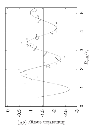
Figure 1: The immersion energy versus jellium sphere radius for jellium spheres of background density $0.007a_{B}^{-3}$. The straight line is the value of the immersion energy for Hydrogen in infinite jellium of the same background density and the sinusoidal line is a guide to the eye. The highlighted points correspond to $N=10$ and $N=50$.

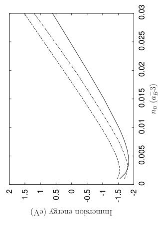
Figure 2: Plots of immersion energy versus background density for a Hydrogen atom immersed in jellium spheres of size 10 (solid curve) and 50 (dashed curve) electrons. Also plotted is the immersion energy curve for a Hydrogen atom in infinite jellium (dot-dash curve).

Our calculations also show that the atom-induced density of the Hydrogen atom in finite jellium tends smoothly towards that of a Hydrogen atom in infinite jellium as the size of the jellium sphere is increased. Figure 3 shows our calculations of the atom-induced densities for a Hydrogen atom in jellium spheres with a background density $0.01a_{B}^{-3}$. We consider jellium spheres with $10$, $50$ and $338$ electrons and also plot the atom-induced density for a Hydrogen atom in infinite jellium. We see clearly that as we increase the number of electrons in the jellium sphere, the atom-induced density approaches the limiting atom-induced density of a Hydrogen atom in infinite jellium.

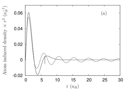
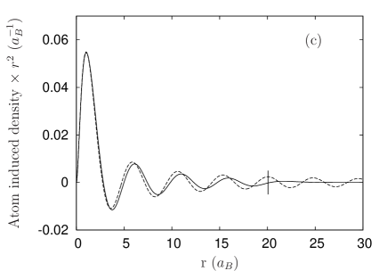
Figure 3: Plots of LSDA atom-induced densities for Hydrogen in finite jellium spheres of background density $0.01a_{B}^{-3}$, with (a) 10, (b) 50 and (c) 338 electrons (solid lines). Also plotted is the atom-induced density for a Hydrogen atom in infinite jellium at the same background density (dashed lines). The jellium sphere radius is shown by a vertical straight line.

III VQMC Solution

III.1 Methodology

In VQMC we use importance sampling to replace the expectation value of the Hamiltonian with a sum over so-called local energies

$$\langle\Psi_{T}|\hat{H}|\Psi_{T}\rangle={1\over{{\cal N}}}\int\Psi_{T}^{*}({\bf R})\hat{H}\Psi_{T}({\bf R})d{\bf R}=$$

$$\int{|\Psi_{T}({\bf R})|^{2}\over{{\cal N}}}{\hat{H}\Psi_{T}({\bf R})\over{\Psi_{T}({\bf R})}}d{\bf R}\approx{1\over{n}}\sum_{i=1}^{n}{\hat{H}\Psi_{T}({\bf R}_{i})\over{\Psi_{T}({\bf R}_{i})}}=\bar{E}$$

where ${\cal N}=\int|\Psi_{T}({\bf R})|^{2}d{\bf R}$, ${\bf R}_{i}$ are sets of particle coordinates, $\{{\bf r}_{1}^{(i)},{\bf r}_{2}^{(i)},\dots,{\bf r}_{N}^{(i)}\}$ (referred to as configurations) which sample the probability distribution ${|\Psi_{T}({\bf R})|^{2}/{{\cal N}}}$ and where $\hat{H}\Psi_{T}({\bf R}_{i})/{\Psi_{T}({\bf R}_{i})}$ is referred to as the local energy, which is summed over a suitably large number of configurations, $n$. These configurations are generated using the Metropolis algorithm.[16]

By the variational principle we know that this expectation value is an upper bound on the exact ground-state energy. To get as close as possible to the ground-state, we minimize $\sigma_{l.e.}$,[17, 18] the standard deviation of the local energy.

The trial wavefunction, $\Psi_{T}$ is written as a product of spin-up and spin-down Slater determinants, $D^{\uparrow}$ and $D^{\downarrow}$, containing LSDA orbitals calculated for the same system. In addition the wavefunction contains a Jastrow factor [19] which describes the correlations between the electrons. For our Jastrow factor we use the same as that used by Sottile et al. [12] in their calculations of jellium spheres (they did not include an embedded atom), except for a ’multipolar’ term which we do not include in our calculations. The trial wavefunction is

$$\Psi_{T}({\bf r}_{1},\cdots,{\bf r}_{N})=\exp\left[\sum_{i=1}^{N}\left(\sum_{n=1}^{6}\alpha_{n}^{(i)}j_{0}\left({n\pi r_{i}\over{R_{jell}}}\right)\right)\right]$$

$$\times\exp\left[\sum_{1\leq i<j\leq N}\frac{1}{2}\left({{a_{ij}r_{ij}+b_{ij}{r_{ij}}^{2}}\over{1+c_{ij}(r_{i})r_{ij}+d_{ij}{r_{ij}}^{2}}}+\right.\right.$$

$$\left.\left.{{a_{ij}r_{ij}+b_{ij}{r_{ij}}^{2}}\over{1+c_{ij}(r_{j})r_{ij}+d_{ij}{r_{ij}}^{2}}}\right)\right]$$

$$\times D^{\uparrow}({\bf r}_{1},\cdots,{\bf r}_{N/2})D^{\downarrow}({\bf r}_{N/2+1},\cdots,{\bf r}_{N})$$

where $c_{ij}$ is given by

$$c_{ij}(r_{i})=c_{ij}^{0}+c_{ij}^{1}\arctan[(r_{i}^{2}-R_{jell}^{2})/2\bigtriangleup R_{jell}]$$

Parameters $a_{ij}$, $b_{ij}$, $c_{ij}^{0}$, $c_{ij}^{1}$ and $d_{ij}$ depend only on the relative spins of electrons $i$ and $j$ and $\alpha_{n}^{(i)}$ depend only on the spin of electron $i$. The parameters $a_{ij}$ are determined by the electron-electron cusp condition. Note that the nuclear-electron cusp condition is automatically satisfied on account of the LSDA orbitals in the determinant. The other 15 parameters in the Jastrow factor are variational parameters which are varied in order to minimize $\sigma_{l.e.}$. Correlated sampling [3, 20, 21] is used in the minimization procedure, which avoids the need to recalculate new configurations for each set of Jastrow parameters.

III.2 Fixing the jellium sphere size

The number of electrons in the jellium sphere is chosen so that the immersion energy is as close to that of the atom in infinite jellium as possible. In addition, in order to have a good trial wavefunction we require a number of electrons such that it is possible to choose a configuration of the electrons in the open-shell so as to give a purely real wavefunction overall. The VQMC energy is also minimized by choosing configurations which are as non-magnetic as possible. With these considerations in mind, and also with a view to minimize computational effort, we choose a 10-electron jellium sphere for the calculations presented below. This choice leads to the following VQMC electron configuration for the Hydrogen in jellium

$$1s^{1\uparrow},1s^{1\downarrow},2s^{1\uparrow},2s^{1\downarrow},2p^{3\uparrow},2p^{3\downarrow},3d^{1\uparrow}$$

and the configuration for the 10-electron jellium sphere without the Hydrogen atom

$$1s^{1\uparrow},1s^{1\downarrow},2p^{3\uparrow},2p^{3\downarrow},3d^{\uparrow},3d^{\downarrow}$$

where the $d$ electrons are placed in orbitals with magnetic quantum number, $m=0$.

In the LSDA solution for the 10-electron jellium sphere, the two $3d$ electrons are instead filled as $3d^{2\uparrow}$ in order to minimize the total energy, in a manner consistent with Hund’s rule. Note that the $d$ sub-shell is not full and so the density contribution from these electrons is spherically symmetrized in LSDA before recalculating the KS potentials.

IV SIC Solution

In our SIC calculations, the SIC will not be applied to all electrons in the system. Instead we apply SIC only to the $1s$ spin-up and spin-down electrons. This approach is taken because our Hydrogen atom in a jellium sphere is meant to be an approximation of Hydrogen in infinite jellium, and in the latter, only the $1s^{\uparrow}$ and $1s^{\downarrow}$ electrons are sufficiently localized to warrant the correction. Hence for our SIC solution, the $1s$ electrons will obey KS equations with a SI-corrected potential and all the other electrons obey the standard LSDA KS equations.

For our 10-electron jellium sphere, the $1s$ and $2s$ orbitals of a given spin are calculated from different eigenvalue equations (unlike in the LSDA, where both share the same potential) and so will not in general be orthogonal. However, the KS formulation of DFT requires this orthogonality and so it must now be imposed, for which we use Gram-Schmidt orthogonalization [22]

$$\psi_{2s}^{\sigma,orth}(r)={\cal{N}}^{\sigma}\left(\psi_{2s}^{\sigma}(r)-\int\psi_{1s}^{\sigma*}(r^{\prime})\psi_{2s}^{\sigma}(r^{\prime})d{\bf r}^{\prime}\psi_{1s}^{\sigma}(r)\right)$$

where $\cal{N}^{\sigma}$ ensures the correct normalization of the orbitals.

The SIC energy functional is

$$E=\sum_{n\neq 2,l,m,\sigma}\int{\psi_{nlm}^{\sigma*}}({\bf r})(-\frac{1}{2}\nabla^{2}){\psi_{nlm}^{\sigma}}({\bf r})d{\bf r}+$$

$$\sum_{\sigma}\int{\psi_{2s}^{\sigma,orth*}}({\bf r})(-\frac{1}{2}\nabla^{2}){\psi_{2s}^{\sigma,orth}}({\bf r})d{\bf r}+$$

$$\sum_{m,\sigma}\int{\psi_{2p,m}^{\sigma*}}({\bf r})(-\frac{1}{2}\nabla^{2}){\psi_{2p,m}^{\sigma}}({\bf r})d{\bf r}+$$

$$\frac{1}{2}\int\int{n(r)n(r^{\prime})\over{|{\bf r}-{\bf r}^{\prime}|}}d{\bf r}d{\bf r}^{\prime}+\int v_{ext}(r)n(r)d{\bf r}+E_{xc}[n^{\uparrow},n^{\downarrow}]-$$

$$\sum_{\sigma}\left[\frac{1}{2}\int\int{n_{1s}^{\sigma}(r)n_{1s}^{\sigma}(r^{\prime})\over{|{\bf r}-{\bf r}^{\prime}|}}d{\bf r}d{\bf r}^{\prime}+E_{xc}[n_{1s}^{\sigma},0]\right]+$$

$$Z\int_{r=0}^{r=R_{jell}}{n_{0}\over{r}}d{\bf r}+\frac{3}{5}{N^{5/3}\over{r_{s}}}$$

Note that the $2s$ contribution to the kinetic energy is most easily calculated by evaluating the radial derivatives of the orbitals. The alternative method of substituting in from the KS equations is also possible, but is more complicated in this case as the orthogonalized orbitals are now mixtures of the eigenstates of the KS equations. As with the LSDA results, both methods are found to give the same results.

V Results

V.1 Total energies and immersion energies

We report VQMC solutions for a Hydrogen atom immersed in 10-electron jellium spheres of background densities $0.001a_{B}^{-3}$ through to $0.03a_{B}^{-3}$ ($r_{s}$ values of $6.2$ and $2$ respectively). Total energies were calculated and are presented, along with LSDA and SIC results, in Fig. 4. Total energies are also calculated using a close approximation to the Hartree-Fock method (HF). These points are calculated by evaluating the expectation value of the Hamiltonian for a wavefunction consisting of just the Slater determinant part containing the LSDA orbitals. This is achieved by performing a VQMC run with the Jastrow factor set equal to one.

Energies for jellium spheres but without the Hydrogen atom are presented in Fig. 5. Finally, the immersion energies are reported in Fig. 6.

In calculating the immersion energy for HF, VQMC and SIC the exact value of the Hydrogen atom energy is used, namely $-13.606eV$. This is appropriate as calculations using HF and SIC both give this value and in the case of VQMC, the calculation is correct to a very high level of precision. For the LSDA calculation, the atom energy is found to be $-13.030$eV.

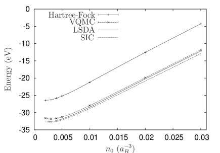
Figure 4: Total energy of a Hydrogen atom immersed in a 10-electron jellium sphere for different background densities.

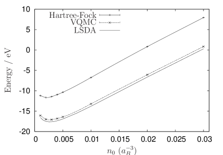
Figure 5: Total energy of a 10-electron jellium sphere for different background densities.

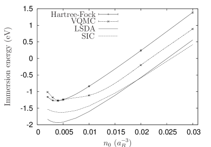
Figure 6: Immersion energies for a Hydrogen atom immersed in a 10-electron jellium sphere for different background densities.

The total energy curves calculated using the different methods are all of the same shape and feature minima at roughly the same locations. The LSDA, SIC and VQMC curves lie within $1eV$ of one another in the atom in jellium total energy graph and similarly the LSDA and VQMC curves are within $1eV$ of one another in the jellium sphere total energy graph. HF gives total energy curves for the atom in jellium and for the jellium sphere which are rigidly shifted by about $5$eV above the VQMC curves.

We note that our VQMC total energy curve for the jellium sphere is slightly different to the type obtained by Sottile et al.[12] Their VQMC results were found to be slightly lower than the LSDA results above background densities of about $0.01a_{B}^{-3}$. This is because we neglected to include the ’multipolar’ term in the trial wavefunction which Sottile et al. [12] used in their calculations. In their work, this term was found to improve the VQMC solution for the larger background densities, but was relatively unimportant at densities near the minimum.

When the total energy curves are subtracted from one another to give the immersion energy curves, the large error in the HF calculations cancel out. We find all four curves lie within $1$eV of one another and all curves feature a minimum at approximately $0.004a_{B}^{-3}$. Notice that the LSDA results for the immersion energy curve are lower than the VQMC results, which means that the LSDA is overbinding the atom to the jellium relative to VQMC.

Calculations by Sugiyama et al. [11] of the immersion energy has a discrepancy of 5eV between Monte Carlo and LSDA, which is very much larger than we find here. Possibly this difference was because of a different choice of trial wavefunction.

We see that the VQMC immersion energy curve below $0.005a_{B}^{-3}$ is more closely followed by the SIC curve than by the LSDA curve. If we regard our VQMC results as a benchmark (see Section VI for a discussion of this) then this indicates that the SIC is outperforming the LSDA for these background densities. This is expected as the $1s$ bound states are becoming more localized at these low background densities and therefore the self-interaction of these bound states is increasing.

Note that for an atom in infinite jellium the SIC and LSDA curves would begin to coincide at large background densities due to the $1s$ electrons becoming increasingly delocalized. However for our system of an atom in finite jellium this is not the case. As the background density is increased, the sphere size becomes smaller and so effects due to the finite size of our system begin to impinge on the results.

V.2 Atom-induced densities

Atom-induced densities (multiplied by $r^{2}$) are plotted in Fig. 7 for a background density of 0.004$a_{B}^{-3}$. The Hydrogen-like maximum in the atom-induced density is very similar between VQMC and LSDA for $r$ less than $4a_{B}$. A discrepancy of at most 5% is identified in this region. On the other hand, as highlighted by Hoffman and Pratt,[23] the work of Sugiyama et al. [11] shows a difference of 30% between LDA and VQMC atom-induced densities near the proton. The much smaller discrepancy in our results is probably due to our use of a trial wavefunction which performs better than that of Sugiyama et al. close to the proton.

However, our atom-induced density plots show the same discrepancy in the Friedel oscillation between LSDA and VQMC as was seen by Sugiyama et al.[11, 23] In particular the minimum in the atom-induced density for the LSDA is much deeper than that for the VQMC. Also the wavelength of the oscillation is larger for VQMC and so the Friedel oscillation maximum occurs at a larger radius.

The SIC atom-induced density is also included in Fig. 7. The SIC and LSDA densities are essentially identical, which seems unusual given the difference in the immersion energies for these methods.

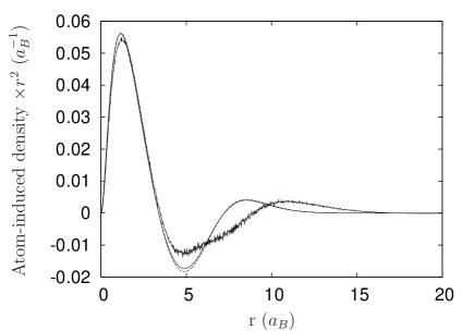
Figure 7: Atom-induced density as calculated using the different methods, for $n_{0}=0.004a_{B}^{-3}$. The solid line is the LSDA density, the dashed line is the SIC density and the noisy line is the VQMC density.

VI Conclusions

We have presented what we believe to be the first reliable VQMC results for the atom in jellium model system. The immersion energy versus background density curves for VQMC, LSDA and SIC lie within $1eV$ of each other with minimas in approximately the same positions. The LSDA results show an overbinding of the atom to the jellium relative to the VQMC result. Viewing the VQMC as a benchmark, this is consistent with the general overbinding seen in LSDA. In addition, for low background densities, the immersion energy curve of VQMC is more closely followed by the the SIC immersion energy curve than by the LSDA immersion energy curve. Again, viewing VQMC as a benchmark, this is consistent with the fact that the SIC is expected to be more accurate than the LSDA for systems with more strongly localized electrons (as is the case for the low background densities).

The status of the VQMC results as a benchmark is uncertain however. More accurate DQMC calculations would yield lower total energies of both the atom in jellium and the jellium relative to the VQMC results. However, because the immersion energy is calculated as the difference between these energies, part of the change in going from VQMC to DQMC will cancel out when we calculate the immersion energy. Furthermore, Sottile et al. [12] found a rigid shift of only $-0.2$eV in the DQMC energies of an 8-electron jellium sphere relative to the VQMC energies. This suggests that our results for the immersion energy would not be strongly modified by using DQMC.

References

- [1] K. W. Jacobsen, J. K. Nørskov, and M. J. Puska. Phys. Rev. B, 35:7423, 1987.
- [2] K. W. Jacobsen. Many-Atom Interactions in Solids, Springer Proceedings in Physics Vol. 48. Springer, Berlin, 1990, pg. 34.
- [3] W. M. C. Foulkes, L. Mitas, R. J. Needs, and G. Rajagopal. Rev. Mod. Phys., 73:33, 2001.
- [4] D. Ceperley, G. V. Chester, and M. H. Kalos. Phys. Rev. B, 16:3081, 1977.
- [5] P. Hohenberg and W. Kohn. Phys. Rev., 136:B864, 1964.
- [6] W. Kohn and L. J. Sham. Phys. Rev., 140:A1133, 1965.
- [7] R. Dreizler and E. Gross. Density Functional Theory. Plenum Press, New York, 1995.
- [8] O. Gunnarsson, B. I. Lundqvist, and J. W. Wilkins. Phys. Rev. B, 10:1319, 1974.
- [9] U. von Barth and L. Hedin. J. Phys. C, 5:1629, 1972.
- [10] J. P. Perdew and A. Zunger. Phys. Rev. B, 23:5048, 1981.
- [11] G. Sugiyama, L. Terray, and B. J. Alder. J. Stat. Phys., 52:1221, 1988.
- [12] F. Sottile and P. Ballone. Phys. Rev. B, 64:045105, 2001.
- [13] A. Hintermann and M. Manninen. Phys. Rev. B, 27:7262, 1983.
- [14] M. J. Puska and R. M. Nieminen. Phys. Rev. B, 43:12221, 1991.
- [15] A. I. Duff. PhD thesis, University of Bristol, 2007.
- [16] N. Metropolis, A. W. Rosenbluth, M. N. Rosenbluth, A. H. Teller, and E. Teller. J. Chem. Phys., 21:1087, 1953.
- [17] C. J. Umrigar, K. G. Wilson, and J. W. Wilkins. Phys. Rev. Lett., 60:1719, 1988.
- [18] R. L. Coldwell. Int. J. Quantum Chem., Quantum Chem. Symp., 11:215, 1977.
- [19] R. Jastrow. Phys. Rev., 98:1479, 1955.
- [20] R. L. Coldwell and R. E. Lowther. Int. J. Quantum Chem. Syrup., 12:329, 1978.
- [21] Y. Kwon, D. M. Ceperley, and R. M. Martin. Phys. Rev. B, 50:1684, 1994.
- [22] G. Arfken. Mathematical Methods for Physicists, 3rd ed, pp. 516-520. Academic Press, 1985.
- [23] G. G. Hoffman and L. R. Pratt. Mol. Phys., 82:245, 1994.
- [24] J. P. Perdew and A. Zunger. Phys. Rev. B, 23:5048, 1981.
- [25] O. Gunnarsson and B. I. Lundqvist. Phys. Rev. B, 13:4274, 1976.
- [26] D. D. Johnson. Phys. Rev. B, 38:12807, 1988.
- [27] M. H. Hettler, M. Mukherjee, M. Jarrell, and H. R. Krishnamurthy. Phys. Rev. B, 61:12739, 2000.