Collisions between equal sized ice grain agglomerates

Abstract

Context. Following the recent insight in the material structure of comets, protoplanetesimals are assumed to have low densities and to be highly porous agglomerates. It is still unclear if planetesimals can be formed from these objects by collisional growth.

Aims. Therefore, it is important to study numerically the collisional outcome from low velocity impacts of equal sized porous agglomerates which are too large to be examined in a laboratory experiment.

Methods. We use the Lagrangian particle method Smooth Particle Hydrodynamics to solve the equations that describe the dynamics of elastic and plastic bodies. Additionally, to account for the influence of porosity, we follow a previous developed equation of state and certain relations between the material strength and the relative density.

Results. Collisional growth seems possible for rather low collision velocities and particular material strengths. The remnants of collisions with impact parameters that are larger than 50 % of the radius of the colliding objects tend to rotate. For small impact parameters, the colliding objects are effectively slowed down without a prominent compaction of the porous structure, which probably increases the possibility for growth. The protoplanetesimals, however, do not stick together for the most part of the employed material strengths.

Conclusions. An important issue in subsequent studies has to be the influence of rotation to collisional growth. Moreover, for realistic simulations of protoplanetesimals it is crucial to know the correct material parameters in more detail.

1 Introduction

The initial growth of particles in a protoplanetary disc is accomplished by sticking collisions. All solid objects in a planetary system are believed to have been developed from collisions between small dust particles with initial sizes of about $0.1$ micron (Greenberg, 1982). These collisions result from Brownian motion, gas turbulence in the disc and gas drag (Weidenschilling, 1977; Voelk et al., 1980; Weidenschilling & Cuzzi, 1993). It has been shown that even protoplanetesimals of equal mass might have rather high relative velocities due to different shapes and hence different gas resistances (Benz, 2000), depending on the orbital distance to the protostar. Experimental data for collisional growth of macroscopic agglomerates with sizes extending the dm-regime are rather scarce. The formation of such macroscopic bodies from smaller dust grains was studied in detail by Ossenkopf (1993) and the fractal growth was modelled by Dominik & Tielens (1997) and Kempf et al. (1999). Generally, the dust particles stick together due to van-der-Waals forces. This growth process leads to (highly) porous agglomerates, a fact that was experimentally confirmed by Wurm & Blum (1998). These macroscopic agglomerates do not stick together as easily as tiny dust grains which only interact by van-der-Waals forces. Instead, aggregate compaction, fragmentation and disruption become important above a specific kinetic energy of the collision. The agglomerates can break and can be dispersed which eventually prevents a fast growth process or even further growth at all. It is now generally assumed that decimetre sized porous agglomerates can form rather quickly in the presolar nebula and the protoplanetary accretion disc (Poppe et al., 2000; Wurm & Blum, 1998; Blum & Wurm, 2000; Weidenschilling, 2000). The critical bottleneck in the formation process of planetesimals lies however in the size range from about several decimetre to objects whose interaction is mainly dominated by gravitation, that is 1 to 10 $\mathrm{km}$ planetesimals. First studies to the collisional growth of brittle planetesimals with material strength were performed by Benz & Asphaug (1994, 1995, 1999) and Benz (2000). Their results indicate that the weakest bodies during collisions are in the size range from metres to around 100 $\mathrm{m}$. Caused by the stronger interaction with the gas, metre sized bodies experience higher collision velocities and are also rather fragile objects and easily disrupted.

A better understood problem is the formation of planets from planetesimals. The formation of planetary embryos or cores has been investigated in a series of publications (Stewart & Wetherill, 1988; Wetherill & Stewart, 1989, 1993) with the application of a statistical approach to describe the evolution of a swarm of planetesimals around the star. Later, by the use of modern supercomputers, direct n-body simulations of a large number of planetesimals became feasible and yielded similar results (Kokubo & Ida, 2000, 2002). Once planetary cores have formed, the terrestrial planets grow through collisions between them (Chambers & Wetherill, 1998; Agnor et al., 1999; Kominami & Ida, 2002). In this size regime, the collisional outcome is by far dominated by gravitational interactions (e.g., Agnor & Asphaug, 2004).

One alternative to avoid the bottleneck at the metre length scale of the formation process of planetesimals is gravitational instability of the dust layer in the midplane of the protoplanetary accretion disc. This idea was suggested independently by Safronov (1969) and Goldreich & Ward (1973). For the solar nebula, Goldreich & Ward (1973) found gravitational clumping of the dust which forms clumps with radii of 10 $\mathrm{km}$ at 1 $\mathrm{AU}$ within 1000 years after the onset of the vertical settling of dust. However, it is still unclear and strongly discussed in the community whether the dust in the midplane can become gravitational unstable, because Kelvin-Helmholtz instability and turbulent motion of dust particles in the disc lead to significant velocity dispersions which may prevent the collapse (Cuzzi et al., 1993; Weidenschilling, 2000; Youdin & Shu, 2002; Youdin & Chiang, 2004).

Therefore, collisional growth of metre sized bodies has to be studied in greater detail in order to investigate the mechanisms of planetesimal formation. Laboratory experiments of collisions between water ice objects (e.g., Bridges et al., 1996) have been restricted to smaller sizes (up to several $\mathrm{cm}$) and low impact velocities (up to several $\mathrm{cm/s}$). Thus, experiments have concentrated on the dependence of sticking forces from the frost-coating of the surfaces (Supulver et al., 1997) or on measuring restitution coefficients (Supulver et al., 1995).

Since real collisions between objects of metre size are not feasible yet in laboratory experiments, one has to resort to numerical simulations. Here, we employ the numerical Lagrangian particle method Smooth Particle Hydrodynamics (SPH) which was first introduced by Lucy (1977) and Gingold & Monaghan (1977) for modelling compressible flows in astrophysical problems. The method was extended to solid state mechanics in the beginning of the nineties by Libersky & Petschek (1990) and improved extensively in the following years (Libersky et al., 1993; Randles & Libersky, 1996; Libersky et al., 1997). After Benz (2000) has applied the method successfully to simulations of low velocity collisions between brittle objects, Sirono (2004) used experimentally measured data to parametrise the compressive strength curve of icy grain agglomerates and derived a modified Murnaghan equation of state (see sect. 2) to simulate porous objects.

Recent astronomical investigations such as the Deep Impact mission (Lisse et al., 2006) and observations of comets (e.g., Lamy et al. 2006) yield strong indications for rather low densities of comets (the values range from 0.1 $\mathrm{g/cm^{3}}$ to several tenths of $\mathrm{g/cm^{3}}$ and still have some larger errors). This matches fairly well with the idea of collisional growth of fractal porous dust agglomerates to planetesimals.

In order to extend the investigations by Sirono (2004), we apply his model to simulate the collisions between equal sized (ice) agglomerates with different impact parameters and also explore the influence of material properties to the simulation outcome. The outline of the paper is as follows: In the next section, we will present the physical model, that is the basic equations and material properties we assume. In sect. 3 we will discuss some numerical issues and in sect. 4 the setup of our simulations. We present our results in sect. 5 and finally draw some conclusions.

2 Physical Model

2.1 Basic Equations

The system of partial differential equations that describe the dynamics of an elastic solid body is given by three equations. The first is the continuity equation

$$\frac{\mathrm{d}\varrho}{\mathrm{d}t}+\varrho\frac{\partial v^{\alpha}}{\partial x^{\alpha}}=0,$$ (1)

where $\varrho$ denotes the density and $\mathbf{v}$ the velocity and where the Einstein summation rule is applied. Greek indices denote the spatial coordinates and run from 1 to 3. The second equation in the system accounts for the conservation of momentum

$$\frac{\mathrm{d}v^{\alpha}}{\mathrm{d}t}=\frac{1}{\varrho}\frac{\partial\sigma^{\alpha\beta}}{\partial x^{\beta}}.$$ (2)

The stress tensor $\sigma$ is given by the pressure $p$ and the deviatoric stress tensor $S^{\alpha\beta}$ according to

$$\sigma^{\alpha\beta}=-p\delta^{\alpha\beta}+S^{\alpha\beta}.$$ (3)

In contrast to fluid dynamics, this set of partial differential conservation equations is not sufficient to describe the elastic body, since the time evolution of the deviatoric stress tensor is not yet specified. The missing relations are called the constitutive equations which describe the rheology of the body and relate the kinematic states of the body to the dynamic states. The elastic behaviour of a solid body can be described by Hooke’s law, which reads in three dimensions

$$S^{\alpha\beta}\sim 2\mu\left(\varepsilon^{\alpha\beta}-\frac{1}{3}\delta^{\alpha\beta}\varepsilon^{\gamma\gamma}\right),$$ (4)

where $\mu$ is the shear modulus of the material, and $\varepsilon^{\alpha\beta}$ denotes the strain tensor which is given by

$$\varepsilon^{\alpha\beta}=\frac{1}{2}\left(\frac{\partial x^{\prime\alpha}}{\partial x^{\beta}}+\frac{\partial x^{\prime\beta}}{\partial x^{\alpha}}\right).$$ (5)

Here, the primed coordinates denote the coordinates of the deformed body.

The stress rate has to be defined in a way that obeys the principle of frame invariance. There are various possibilities to achieve this. We follow the usual approach which is used for SPH codes (Benz & Asphaug, 1994) and adopt the Jaumann rate form, where the time evolution of the deviatoric stress tensor can be expressed as

$$\frac{\mathrm{d}S^{\alpha\beta}}{\mathrm{d}t}=2\mu\left(\dot{\varepsilon}^{\alpha\beta}-\frac{1}{3}\delta^{\alpha\beta}\dot{\varepsilon}^{\gamma\gamma}\right)+S^{\alpha\gamma}R^{\gamma\beta}+S^{\beta\gamma}R^{\gamma\alpha},$$ (6)

where $R^{\alpha\beta}$ denotes the rotation rate tensor

$$R^{\alpha\beta}=\frac{1}{2}\left(\frac{\partial v^{\alpha}}{\partial x^{\beta}}-\frac{\partial v^{\beta}}{\partial x^{\alpha}}\right),$$ (7)

and $\dot{\varepsilon}^{\alpha\beta}$ the strain rate tensor

$$\dot{\varepsilon}^{\alpha\beta}=\frac{1}{2}\left(\frac{\partial v^{\alpha}}{\partial x^{\beta}}+\frac{\partial v^{\beta}}{\partial x^{\alpha}}\right).$$ (8)

The closure of this set of equations is provided by the equation of state that relates the pressure $p$ to the density of the agglomerate. Here, we focus on porous objects and follow the semi-empirical approach by Sirono (2004). We use an extension of the Murnaghan equation of state which accounts for the change of porosity and reads

$$p(\varrho)=\left\{\begin{array}[]{ll}K(\varrho_{0}^{\prime})(\varrho/\varrho_{0}^{\prime}-1),&\varrho<\varrho_{\mathrm{c}},\\[4.30554pt] \Sigma(\varrho),&\varrho\geq\varrho_{\mathrm{c}}.\end{array}\right.$$ (9)

The quantity $\varrho_{0}^{\prime}$ is the reference density of an agglomerate at no external stress while $\varrho_{0}$ is the initial density of the porous agglomerate. Note that $\varrho_{0}^{\prime}$ is in general different to the initial density $\varrho_{0}$ of the porous agglomerate after the start of the simulation. The critical density $\varrho_{\mathrm{c}}$ is a function of the reference density $\varrho_{0}^{\prime}$ and determines the state where the pressure reaches the compressive strength limit $\Sigma(\varrho)$. As soon as the pressure decreases, the behaviour of the agglomerate is again elastic but with a different bulk modulus $K(\varrho_{0}^{\prime})$ since the reference density has changed. The slope of $K(\varrho_{0}^{\prime})$ has to be known either by experimental data or theoretical considerations. The tensile strength of the material is determined accordingly and limits the tension for negative pressure.

The sound speed of the agglomerate is given by the bulk modulus of the agglomerate and the reference density according to the relation

$$c(\varrho_{0}^{\prime})=\sqrt{K(\varrho_{0}^{\prime})/\varrho_{0}^{\prime}}.$$ (10)

For plastic states when the pressure exceeds the compressive strength of the material the sound speed is calculated according to

$$c(\varrho)=\sqrt{\frac{\mathrm{d}\Sigma(\varrho)}{\mathrm{d}\varrho}}.$$ (11)

Sirono (2004) additionally uses an empirical damage model for porous agglomerates which is based on the damage model for brittle materials developed for SPH by Benz & Asphaug (1994, 1995). However, this model is only applicable for the simulation of brittle fracture in rocks (Grady & Kipp, 1980), and our test simulations show that the application of the damage model to porous agglomerates does not yield reliable results since the model also includes compressive damage effects. Because of these considerations, we do not include any damage model in our calculations and only consider the fragmentation due to plastic flow.

2.2 Material properties

The shape of the compressive and tensile strength curves have to be known either by experimental data or theoretical considerations. Since we want to compare our calculations to Sirono (2004), we primarily use the values published in his paper which are derived from experimental data (see Kendall et al. 1987; Valverde et al. 1998): The compressive strength is given by $\Sigma(\varphi)=\Sigma_{0}\varphi^{\alpha}$, with $\varphi=\varrho/\varrho_{0}$, and the tensile strength accordingly by $T(\varphi)=T_{0}\varphi^{\beta}$. The dependence of the bulk modulus of the aggregate on the porosity reads $K(\varphi)=K_{0}\varphi^{\gamma}$. The shear modulus is assumed to be $\mu=K/2$, and the shear strength is defined by $Y(\varphi)=\sqrt{2T(\varphi)\Sigma(\varphi)/3}$. The parameter $\varphi$ is related to the porosity $\phi=\varrho/\varrho_{\mathrm{s}}$ in the following way

$$\varphi=\frac{\varrho}{\varrho_{0}}=\phi\frac{\varrho_{\mathrm{s}}}{\varrho_{0}}=\frac{\phi}{\phi_{0}},$$ (12)

where $\varrho_{\mathrm{s}}$ denotes the density of the solid material in the porous body and $p_{0}$ is the porosity of the body at the initial simulation time.

The transition from an elastic state to a yield state of a material can be characterised by a complex stress state. The stress at which the transition starts is called the yield stress and the condition is called the yield criterion or the plasticity criterion. In this paper, we follow the implementation by Benz & Asphaug (1995) and assume isotropic material and apply the von Mises yield criterion: We calculate the second irreducible invariant of the deviatoric stress tensor $J_{2}=S_{\alpha\beta}S^{\alpha\beta}$ and reduce the deviatoric stress when necessary according to

$$S^{\alpha\beta}\rightarrow fS^{\alpha\beta},\qquad f=\min\left[Y(\varphi)^{2}/3J_{2},1\right].$$ (13)

3 Numerical Issues

Smooth Particle Hydrodynamics (SPH) is perfectly suitable for the simulation of brittle and plastic materials. The continuum of the solid body is discretised into mass packages which are called particles. The particles move like point masses according to the Lagrangian form of the equation of motion. They carry all physical properties like mass, momentum and energy of the part of the solid body they represent. The particles interact by kernel interpolation during the simulation to exchange momentum and energy. For a complete description of the method and its features and qualities, we refer to two comprehensive review articles (Benz, 1990; Monaghan, 1992).

In standard SPH, the velocity derivatives in eqs. (7) and (8) for the determination of the rotation rate and the strain rate tensor for particle $i$ are usually calculated according to

$$\frac{\partial v_{i}^{\alpha}}{\partial x_{i}^{\beta}}=\sum_{j}\frac{m_{j}}{\varrho_{j}}(v^{\alpha}_{j}-v^{\alpha}_{i})\frac{\partial W^{ij}}{\partial x^{\beta}_{i}},$$ (14)

where the sum runs over all interaction partners $j$ of particle $i$, and $W^{ij}$ denotes the kernel for the particular interaction.

This approach, however, leads to erroneous results and does not conserve angular momentum due to the discretisation error by particle disorder in simulations of solid bodies. This error can be avoided by constructing and applying a correction tensor $C^{\gamma\beta}$ according to

$$\frac{\partial v_{i}^{\alpha}}{\partial x_{i}^{\beta}}=\sum_{j}\frac{m_{j}}{\varrho_{j}}(v^{\alpha}_{j}-v^{\alpha}_{i})\sum_{\gamma}\frac{\partial W^{ij}}{\partial x^{\gamma}_{i}}C^{\gamma\beta},$$ (15)

where the correction tensor $C^{\gamma\beta}$ is the inverse of

$$\sum_{j}\frac{m_{j}}{\varrho_{j}}(x^{\alpha}_{j}-x^{\alpha}_{i})\frac{\partial W^{ij}}{\partial x^{\gamma}_{i}},$$ (16)

that is

$$\sum_{j}\frac{m_{j}}{\varrho_{j}}(x^{\alpha}_{j}-x^{\alpha}_{i})\sum_{\gamma}\frac{\partial W^{ij}}{\partial x^{\gamma}_{i}}C^{\gamma\beta}=\delta^{\alpha\beta}.$$ (17)

By applying this correction tensor first order consistency can be constructed where the errors due to particle disorder cancel out and the conservation of angular momentum is ensured. This is similar to an approach that Bonet & Lok (1999) proposed for the conservation of angular momentum, where all spatial derivatives are corrected according to eq. (15). We have found however that it is sufficient to correct only the rotation rate and the strain rate tensor.

We additionally use the standard SPH artificial viscosity (Monaghan & Gingold, 1983) with $\alpha=1$. However, in order to reduce the viscous energy dissipation, we follow Sirono’s approach and apply the artificial viscosity only when the approaching relative velocity of two particles is larger than the sound speed in contrast to the standard case where the artificial viscosity acts always on approaching particles.

Our SPH code parasph (Hipp & Rosenstiel, 2004) has been successfully tested with some numerical standard tests such as the collision of perfectly elastic rings (Swegle, 1992; Monaghan, 2000) and the simulations of ductile and brittle rods under tension (Benz & Asphaug, 1994; Gray et al., 2001). Additionally, the Sirono model in the extended code has been checked carefully (Schäfer, 2005) and we have successfully reproduced the impact result for the standard setup in Sirono (2004).

4 Setup

All collisions have been simulated in three dimensions. The setup of our calculations includes the following parameters: Two spherical ice agglomerates with the initial density $\varrho_{0}=0.1\leavevmode\nobreak\ \mathrm{g/cm^{3}}$ and identical radius $r=1\leavevmode\nobreak\ \mathrm{m}$ collide at either $20\leavevmode\nobreak\ \mathrm{m/s}$ or $10\leavevmode\nobreak\ \mathrm{m/s}$. The initial density implies an initial porosity of 90 %. The density dependencies of compressive and tensile strengths are chosen according to Sirono (2004) to $\Sigma(\varrho)=\Sigma_{0}(\varrho/\varrho_{0})^{6}$ and $T(\varrho)=T_{0}(\varrho/\varrho_{0})^{5}$, and the bulk modulus is given by $K(\varrho)=K_{0}(\varrho/\varrho_{0})^{4}$. We always assume the shear modulus is given by $\mu=K/2$. For the first simulations with impact velocity $20\leavevmode\nobreak\ \mathrm{m/s}$ we use the basic setup values from Sirono and set $K_{0}=6\times 10^{5}\leavevmode\nobreak\ \mathrm{Pa}$, $\Sigma_{0}=600\leavevmode\nobreak\ \mathrm{Pa}$, and $T_{0}=6\times 10^{3}\leavevmode\nobreak\ \mathrm{Pa}$. These are the values for which Sirono (and we) find perfect sticking behaviour for a smaller sphere impacting into a larger object (with a radii ratio of 10:3) at speed $10\leavevmode\nobreak\ \mathrm{m/s}$. The temperature implicitely assumed in this set of parameters corresponds to very cold ice, which is consistent with the simulation results where large deformations but hardly any compression is found. Since the probability of a head-on collision is low, we have additionally varied the impact parameter of the collision, $b=0.2$, $0.4,$ $0.8$, $1.2\leavevmode\nobreak\ \mathrm{m}$. The results of these simulations are shown in sect. 5.1.

To study the importance of realistic material properties, we have then varied the tensile and compressive strength parameters $T_{0}$ and $\Sigma_{0}$ in some of the $10\leavevmode\nobreak\ \mathrm{m/s}$ head-on collisions and present these calculations in sect. 5.2. Reducing the impact velocity also allows to compare the influence of the latter.

5 Results

5.1 Varying impact parameter

As noted above, in this section we focus on the material parameters for which Sirono (2004) found perfect sticking for a collision with a projectile 3:10 smaller in radius than the target. Figs. 1-5 present the simulation outcome for five different impact parameters. The plots show the SPH particles with a colour-scale code for the density of each particle. As we are mainly interested in the final configuration of the impact after compression has ceased, the density is acting as a measure for any permanent compaction that may have taken place during the compression phase.

Each sphere consists of approximately 11 500 SPH particles which are initially placed on a tetrahedral grid to maximise the number of adjacent and interacting particles and thus to increase the resolution. The figures show the surface of the resulting objects after impact, as the particles are plotted opaque.

The first simulation (see fig. 1) demonstrates the behaviour during a head-on collision with impact parameter $b=0$. In contrast to the sticking mechanism found by Sirono (2004) with the same material properties but different sizes, the two spheres do not penetrate. In fact, they undergo a large change in shape and the two spheres end up as flattened discs. Almost the entire kinetic energy of the impact is dissipated by plastic deformation, and ultimately the two discs are at rest in the barycentric system. Only some particles which were tossed outwards during the compression phase fly away at constant speed.

The picture slightly changes for the simulation with $b=0.2\leavevmode\nobreak\ \mathrm{m}$ (see fig. 2). As in the head-on collision, the two spheres transform into flattened discs with some separate particles floating away. In contrast to the head-on collision, the remnants of the spheres rotate slowly.

First major difference arises at the step from $b=0.2\leavevmode\nobreak\ \mathrm{m}$ to $b=0.4\leavevmode\nobreak\ \mathrm{m}$ (see fig. 3), when the spheres break up. Again, the spheres undergo a large plastic deformation during the compression phase and become strongly prolate. A small piece is quarried out of each object after the compression due to the strong tensile forces caused by rotation.

Even more smaller fragments emerge after the collision with impact parameter $b=0.8\leavevmode\nobreak\ \mathrm{m}$ (see fig. 4). However, now the largest remnants of the collision consist of two rotating half-spheres. The density of the half-spheres is exactly the density of the initial spheres. Essentially they have not been compacted.

The situation hardly changes for $b=1.2\leavevmode\nobreak\ \mathrm{m}$ (see fig. 5). Again, smaller fragments are tossed out from the spheres after the compaction phase. The two formed larger remnants have again the shape of half-spheres, slightly larger than in the simulation with $b=0.8\leavevmode\nobreak\ \mathrm{m}$. The rotation rate and the velocity of the half-spheres is larger than for smaller impact parameters.

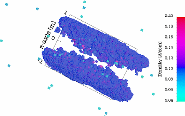
Figure 1: Head-on collision with impact velocity $20\leavevmode\nobreak\ \mathrm{m/s}$. The material strength coefficients are chosen to $\Sigma_{0}=600\leavevmode\nobreak\ \mathrm{Pa}$ and $T_{0}=6000\leavevmode\nobreak\ \mathrm{Pa}$. The plot shows colour-scaled the density for each particle at simulation time $t=0.662\leavevmode\nobreak\ \mathrm{s}$ after contact. The colourbar is in units of $\mathrm{g/cm^{3}}$ and is valid for all colour-scale plots in this paper. Also note that the line of approach is tilted by $\sim 30\degr$ from the vertical in all plots.

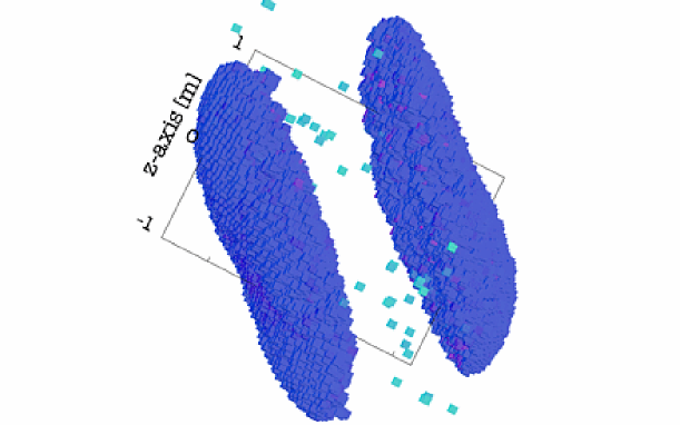
Figure 2: Collision with impact parameter $b=0.2\leavevmode\nobreak\ \mathrm{m}$. The plot shows colour-scaled the density for each particle at simulation time $t=0.662\leavevmode\nobreak\ \mathrm{s}$ after contact.

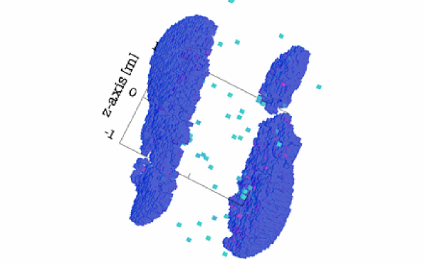
Figure 3: Collision with impact parameter $b=0.4\leavevmode\nobreak\ \mathrm{m}$. The plot shows colour-scaled the density for each particle at simulation time $t=0.662\leavevmode\nobreak\ \mathrm{s}$ after contact.

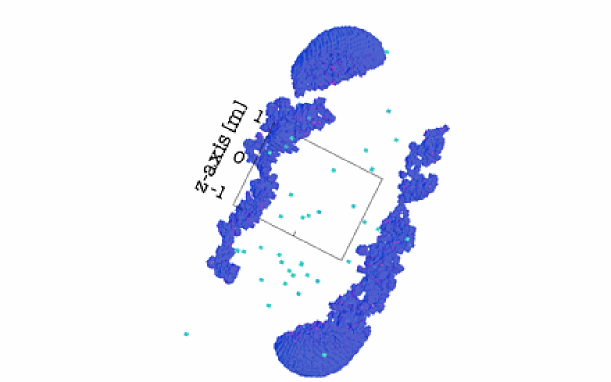
Figure 4: Collision with impact parameter $b=0.8\leavevmode\nobreak\ \mathrm{m}$. The plot shows colour-scaled the density for each particle at simulation time $t=0.662\leavevmode\nobreak\ \mathrm{s}$ after contact.

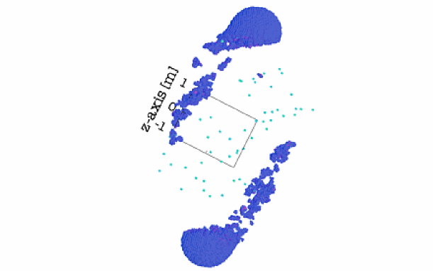
Figure 5: Collision with impact parameter $b=1.2\leavevmode\nobreak\ \mathrm{m}$. The plot shows colour-scaled the density for each particle at simulation time $t=0.662\leavevmode\nobreak\ \mathrm{s}$ after contact.

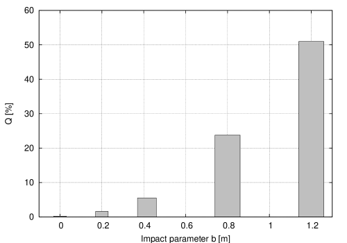
Figure 6: Ratio $Q$ between kinetic energy at end of the simulation and initial energy for five different impact parameters.

The strong influence of the impact parameter $b$ on the change in kinetic energy with the respect to the centre of mass is shown in fig. 6, where the ratio $Q$ of the kinetic energy at the end of the simulation to the initial kinetic energy is plotted. In the case of the head-on collision, more than 99.7 % of the initial kinetic energy has been dissipated during the plastic deformation phase. The remnants (except for a few particles) of the collision are at rest. Although they do not stick together, their relative velocity is zero. Even for impact parameters $b=0.2$ and $0.4$ $\mathrm{m}$, the kinetic energy at the end is less than 10 % of the initial kinetic energy. The spheres are effectively slowed down during the compression phase.

The situation changes for higher impact parameters. For $b=0.8\leavevmode\nobreak\ \mathrm{m}$ less than 80 % and for $b=1.2\leavevmode\nobreak\ \mathrm{m}$ even less than 50 % of the initial kinetic energy is lost due to the compression.

Interestingly, the density of the remnants after the simulation is basically the initial density for all studied impact parameters. Only some small areas in the contact region have a slightly higher density. The density in the interiour of the objects does not differ distinctly from the density at the surfaces. Therefore only the latter is shown in the figures.

5.2 Varying material strength

Although Sirono (2004) has investigated the influence of the material strength on the collisional outcome, we have additionally studied the behaviour for our equal-sized agglomerates.

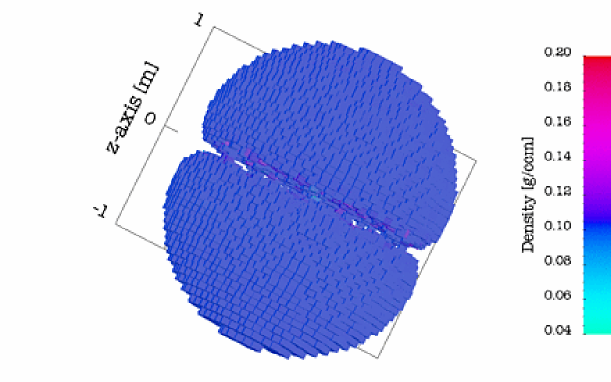
Figure 7: Head-on collision with impact velocity $10\leavevmode\nobreak\ \mathrm{m/s}$. The material strength coefficients are $\Sigma_{0}=600\leavevmode\nobreak\ \mathrm{Pa}$ and $T_{0}=6\,000\leavevmode\nobreak\ \mathrm{Pa}$. The plot shows colour-scaled the density for each particle at simulation time $t=0.5\leavevmode\nobreak\ \mathrm{s}$ after contact.

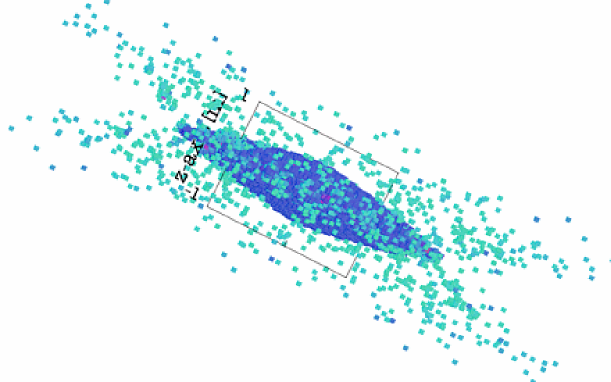
Figure 8: Head-on collision with impact velocity $10\leavevmode\nobreak\ \mathrm{m/s}$. The material strength coefficients are $\Sigma_{0}=600\leavevmode\nobreak\ \mathrm{Pa}$ and $T_{0}=600\leavevmode\nobreak\ \mathrm{Pa}$. The plot shows colour-scaled the density for each particle at simulation time $t=0.5\leavevmode\nobreak\ \mathrm{s}$ after contact.

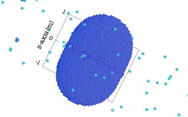
Figure 9: Head-on collision with impact velocity $10\leavevmode\nobreak\ \mathrm{m/s}$. The material strength coefficients are $\Sigma_{0}=6\,000\leavevmode\nobreak\ \mathrm{Pa}$ and $T_{0}=6\,000\leavevmode\nobreak\ \mathrm{Pa}$. The plot shows colour-scaled the density for each particle at simulation time $t=0.5\leavevmode\nobreak\ \mathrm{s}$ after contact.

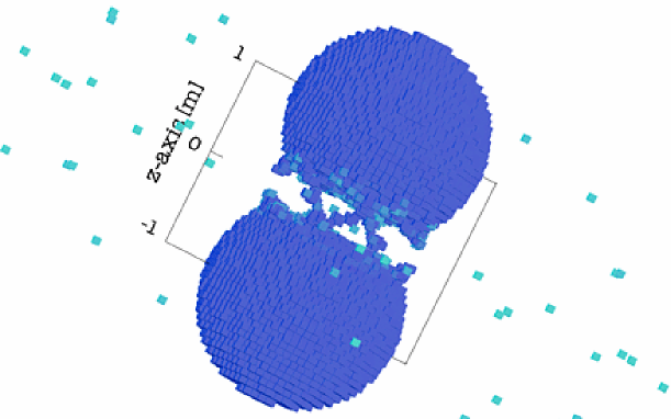
Figure 10: Head-on collision with impact velocity $10\leavevmode\nobreak\ \mathrm{m/s}$. The material strength coefficients are $\Sigma_{0}=60\,000\leavevmode\nobreak\ \mathrm{Pa}$ and $T_{0}=6\,000\leavevmode\nobreak\ \mathrm{Pa}$. The plot shows colour-scaled the density for each particle at simulation time $t=0.5\leavevmode\nobreak\ \mathrm{s}$ after contact.

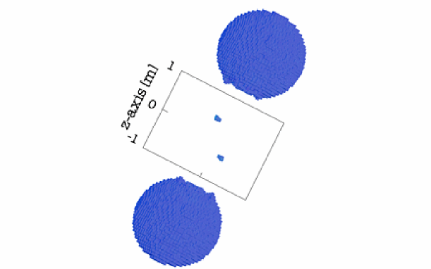
Figure 11: Head-on collision with collision velocity $10\leavevmode\nobreak\ \mathrm{m/s}$. The material strength coefficients are $\Sigma_{0}=60\,000\leavevmode\nobreak\ \mathrm{Pa}$ and $T_{0}=60\,000\leavevmode\nobreak\ \mathrm{Pa}$. The plot shows a colour-scaled the density for each particle at simulation time $t=0.5\leavevmode\nobreak\ \mathrm{s}$ after contact.

All simulations with varying material strengths are head-on collisions with a relative velocity of $10\leavevmode\nobreak\ \mathrm{m/s}$. The basic relations for the compressive and tensile strengths and the bulk modulus remain unchanged, only the coefficients $\Sigma_{0}$ and $T_{0}$ are varied.

The figures 7-10 show colour-scaled density plots of the particles at the end of each simulation. For the first of these simulations, we have used the same material properties as in sect. 5.1, $\Sigma_{0}=600$ $\mathrm{Pa}$ and $T_{0}=6\times 10^{3}\leavevmode\nobreak\ \mathrm{Pa}$ (see fig. 7). Because the collision velocity is half the collision velocity from the simulation shown in fig. 1, the spheres do not experience the same drastic plastic deformation. In fact, they end up as two solid half spheres and no particles were pulled out of the spheres during the compression phase. Their relative velocity at the end are again vanishing. This picture changes drastically if the tensile strength coefficient $T_{0}$ is reduced by one order of magnitude to $600\leavevmode\nobreak\ \mathrm{Pa}$ (see fig. 8). Now the tensile forces are too weak to sustain the bodies during the contact phase. In the end, the two spheres stick together into a disc-like structure and many particles are ejected due to the fragmentation by plastic flow. If the compressive strength parameter $\Sigma_{0}$ is increased to $6\times 10^{3}\leavevmode\nobreak\ \mathrm{Pa}=T_{0}$ instead (see fig. 9), the material is strong enough to evade the fragmentation, only a few particles are thrown out, and the two spheres finally stick together, forming an elongated body. Interestingly, if the compressive strength is augmented even further to $6\times 10^{4}\leavevmode\nobreak\ \mathrm{Pa}$ (see fig. 10), the bodies become too elastic and do not stick. The basic structure of the spheres is conserved, only in the impact contact region, the spheres are flattened. The objects rather bounce off from each other, losing some particles. A nearly fully elastic rebound of the spheres happens for $\Sigma_{0}=T_{0}=6\times 10^{4}\leavevmode\nobreak\ \mathrm{Pa}$ (see fig. 11).

Again, the density of the spheres does not change significantly. Although their shapes change notably, they are not compacted effectively and their porosities stay mainly unchanged.

6 Discussion

The simulations presented in this work extend the investigation of Sirono (2004) to collisions between equal-sized agglomerates. Sirono’s main results regarding collisional growth and stickiness conditions can be summarised in the following way: Porous agglomerates can grow by collisions if the tensile strength is larger than the compressive strength, the shear strength is larger than the compressive strength and the Mach number is lower than $0.04$ for oblique impacts, which corresponds in our simulations to a maximum collision velocity of $3.1\leavevmode\nobreak\ \mathrm{m/s}$. Additionally, a damage restoration effect has to be included, otherwise the agglomerates are totally fragmented. Since we do not use the damage model from Sirono, there is no need for a restoration effect.

Our new simulations with varying impact parameters indicate that collisions with $b<0.4$ lead to drastic shape deformations, the spheres finally form disc-like structures. Clearly, disc-like structures will withstand subsequent collisions even worse if the impact is perpendicular to the disc plane. On the other hand most (for head-on collisions nearly all) of the kinetic energy is lost, which possibly leads to lower collision velocities for following encounters, thus favouring growth in subsequent collisions. The change in shape is lower for larger impact parameters $b>0.4$, where less kinetic energy is lost. However, agglomerates emerging from oblique collisions tend to rotate and eventually break if the tensile strength is not large enough. Then, plastic flow leads to fragmentation of agglomerates after the compression phase. However, the tensile strength of a realistic porous protoplanetesimal might be higher in orders of magnitude than assumed here.

One of the most striking simulation results is the missing compaction of the agglomerates. Although they are rather porous objects (with 90 % porosity), their porosity does not change significantly during the impact. It is unclear, how the porosity in the agglomerates may be reduced and the bodies compacted. Probably, lower collision velocities and differing sizes of the colliding agglomerates lead to the incorporation of smaller bodies into large agglomerates, and a slight decrease of porosity. However, the velocity distribution of protoplanetesimals in the solar nebula at the Earth’s orbital distance ranges up to several tens of $\mathrm{m/s}$. One collision at such a high speed might destroy previous growth entirely.

The varying material strength parameters which were investigated in the second series of simulations show the strong influence of the material properties on the collisional outcome. For the applied values we find the whole spectrum: sticking, no sticking but vanishing relative velocity, complete fragmentation, and elastic rebound. In contrast to Sirono’s results, the only simulation that results in sticking uses $\Sigma_{0}=T_{0}>Y_{0}$. Moreover, since the Mach number of our simulations is $0.13$ for the $10\leavevmode\nobreak\ \mathrm{m/s}$ collisions and $0.26$ for the $20\leavevmode\nobreak\ \mathrm{m/s}$ collisions respectively, all simulations should lead to fragmentation according to Sirono’s results.

Altogether the results indicate that to prevent fragmentation, a large compressive strength may compensate a low tensile strength (see fig. 10) and vice versa (see fig. 7).

7 Conclusion

As long as we do not have more insight into realistic material properties of protoplanetesimals, it is cumbersome to give any accurate description about the formation of planetesimals by collisional growth. However, we have demonstrated that specific strength parameters can lead to growth and encourage the formation of planetesimals even for collisions of equal sized objects, where previous investigations have found destruction. Currently, it is a major topic to establish realistic material parameters of protoplanetesimals in laboratory experiments. Recent experimental data (Blum & Schräpler, 2004; Wurm et al., 2005a, b) provide first insight in the properties of porous dust agglomerates which differ significantly from the properties applied in this study and may lead to further perception. We plan to recalibrate the existing SPH-model which was applied in this paper by performing comparison calculations of impact experiments. Thus, a realistic model for elastic and plastic behaviour of porous agglomerates will be developed.

Additionally, our studies indicate that rotation is an important unexplored effect which needs to be probed in more detail. A subsequent study will therefore focus on the collisions between rotating porous protoplanetesimals.