Clustering by soft-constraint affinity propagation:
Applications to gene-expression data

Abstract

Motivation: Similarity-measure based clustering is a crucial problem appearing throughout scientific data analysis. Recently, a powerful new algorithm called Affinity Propagation (AP) based on message-passing techniques was proposed by Frey and Dueck Frey et al., (2007). In AP, each cluster is identified by a common exemplar all other data points of the same cluster refer to, and exemplars have to refer to themselves. Albeit its proved power, AP in its present form suffers from a number of drawbacks. The hard constraint of having exactly one exemplar per cluster restricts AP to classes of regularly shaped clusters, and leads to suboptimal performance, e.g., in analyzing gene expression data.

Results: This limitation can be overcome by relaxing the AP hard constraints. A new parameter controls the importance of the constraints compared to the aim of maximizing the overall similarity, and allows to interpolate between the simple case where each data point selects its closest neighbor as an exemplar and the original AP. The resulting soft-constraint affinity propagation (SCAP) becomes more informative, accurate and leads to more stable clustering. Even though a new a priori free-parameter is introduced, the overall dependence of the algorithm on external tuning is reduced, as robustness is increased and an optimal strategy for parameter selection emerges more naturally. SCAP is tested on biological benchmark data, including in particular microarray data related to various cancer types. We show that the algorithm efficiently unveils the hierarchical cluster structure present in the data sets. Further on, it allows to extract sparse gene expression signatures for each cluster.

Contact:leone,sumedha,weigt@isi.it

I Introduction

Clustering based on a measure of similarity is a crucial problem which appears throughout scientific data analysis. For an overview see Jain et al., (1999). Recently, a powerful algorithm called Affinity Propagation (AP) based on message passing was proposed by Frey and Dueck Frey et al., (2007). As reported impressively in the original publication, this algorithm achieves a considerable improvement over standard clustering methods like K-means MacQueen, (1967), spectral clustering Shi et al., (2000) and super-paramagnetic clustering Blatt et al., (1996); Shental et al, (2003).

Based on an ad hoc pairwise similarity function between data points, AP seeks to identify each cluster by one of its elements, the so-called exemplar. Each point in the cluster refers to this exemplar, each exemplar is required to refer to itself as a self-exemplar. This hard constraint forces clusters to appear as stars of radius one: There is only one central node, and all other nodes are directly connected to it. Subject to this constraint, AP seeks at maximizing the overall similarity of all data points to their exemplars. The solution to this hard combinatorial task is approximated following the ideas of belief-propagation Yedidia et al., (2005); Kschischang et al., (2001). One of the important points of AP is its computational efficiency: whereas a naive implementation of belief propagation for $N$ data points leads to $O(N^{3})$ messages which have to be determined self-consistently, the elegant formulation of Frey and Dueck allows to work with $O(N^{2})$ messages only. Therefore the algorithm is feasible even in the presence of very large data sets.

Albeit its impressive power in a wide range of applications Frey et al., (2007), AP in its present form suffers from a number of drawbacks. The most important ones related to the present work are:

• The hard constraint in AP relies strongly on cluster-shape regularity: Elongated or irregular multi-dimensional data might have more than one simple cluster center. AP may force division of single clusters into separate ones.

• Since all data points in a cluster must point to the same exemplar, all information about both the internal structure and the hierarchical merging/dissociation of clusters is lost.

• AP has robustness limitations: A small perturbation of similarities may influence the choice of one or few exemplars, and the hard constraint may trigger an avalanche leading to a different partitioning of the data set into clusters. This point is particularly important in the presence of noise in the data as, e.g., in microarray measurements.

• AP forces each exemplar to point to itself. A relaxation of the hard constraint may allow for cluster structures including second- or higher-order pointing processes.

These problems may be solved by modifying the original optimization task of AP. As a first step we relax the hard constraint by introducing a finite penalty term for each constraint violation. This softening can be chosen in a way that the computational complexity of the algorithm remains unchanged, but its performance on biological test sets is improved considerably. Moreover, relaxing the constraint helps in gaining valuable insight into the hierarchical structure of the clustering, increasing result robustness at the same time. By tuning the cluster number we see the merging of two clusters into a single one, or the dissociation of single clusters into two separated ones.

II The Algorithm

Given a set $D=\{x_{\mu}\}_{\mu=1}^{N}$ of $N$ data points, the original algorithm of Frey and Dueck takes as input a collection of real valued similarities $S(\mu,\nu)$ between the pairs $x_{\mu},x_{\nu},\ \mu,\nu\in\{1,...,N\}$. The choice of the similarity measure is heuristic, it depends on the nature of data to be clustered. In the case of high-dimensional data as present in gene-expression analysis, similarity may be measured by the Pearson correlation coefficient or the negative pairwise Euclidean distance. However, for the algorithm described below it is not even necessary that the similarities are symmetric.

The algorithm searches for a mapping ${\bf c}:\{1,...,N\}\mapsto\{1,...,N\}$ which maps each data point $\mu$ to its exemplar $c_{\mu}$ which itself is a data point. This mapping shall minimize the cost function (or energy) $E_{1}[{\bf c}]=-\sum_{\mu=1}^{N}S(\mu,c_{\mu})$ which equals minus the overall similarity of the data points to their exemplars. In the original AP algorithm ${\bf c}$ is restricted by $N$ hard constraints: Whenever a data point is selected as an exemplar by another data point, it has to be its own self-exemplar.

In this setting, we need to specify self-similarities $S(\mu,\mu)$. They describe the availability of data points for being self-exemplars (and thus to serve as a cluster center). Since all data points are a priori equally suitable to play such a role, one is naturally led to choose all self-similarities to have some common value $S(\mu,\mu)\equiv-\sigma,\ \mu=1,...,N$. The free model parameter $\sigma$ acts like a chemical potential in statistical physics, setting the prior likelihood of the number of self exemplars (and of separated clusters consequently). For very small value of $\sigma$, every data point prefers to be its own exemplar, and the number of clusters equals the number of data points. In the opposite extreme case of large $\sigma$, self-exemplars have high cost in $E_{1}[{\bf c}]$. All data points are collected in one large cluster with a single exemplar. For intermediate values $\sigma$ acts as a tuning parameter for the cluster number which decreases monotonously with $\sigma$. Frey and Dueck argue that, if the data set has some underlying structure, the correct clustering can be identified by a comparably broad range of values of the self-similarity in which the inferred cluster structure does not change. If data are not sparse and clusters are symmetrically shaped, then affinity propagation works very well and produces the correct clustering in a very short time.

Finding the cost minimum of $E_{1}[{\bf c}]$ subject to the self-exemplar constraint is a computationally hard task. It can be achieved exactly only for very small systems. The central idea of AP is therefore to identify the exemplars using message passing (belief propagation, BP) as a heuristic strategy Yedidia et al., (2005): Real-valued messages between pairs of data points are updated recursively until a stable clustering emerges. The original AP equations are a direct application of BP (or, equivalently, Max-Sum Kschischang et al., (2001)) to the clustering problem.

There are two types of messages exchanged between data points Frey et al., (2007): The responsibility $r(\mu,\nu)$ is sent from data point $\mu$ to candidate exemplar $\nu$; it reflects the accumulated evidence that $\mu$ chooses $\nu$ as its cluster exemplar. The availability $a(\mu,\nu)$ is sent from candidate exemplar $\nu$ to datum $\mu$; it reflects the appropriateness for $\nu$ to be an exemplar for $\mu$ as a result of the self-exemplar constraint. As mentioned before, the original AP imposes constraints on exemplars to be self-exemplars. We modify the algorithm of Frey and Dueck by softening this hard constraint. We write the constraint attached to a given data point $\mu$ as follows, with $p\in[0,1]$:

$$\chi^{(p)}_{\mu}[{\bf c}]=\left\{\begin{array}[]{lll}p&{\rm if}&\exists\nu:~{}c_{\nu}=\mu,~{}c_{\mu}\neq\mu\\[2.84544pt] 1&{\rm else.}&\end{array}\right.$$ (1)

The first case assigns a penalty $p$ if data point $\mu$ is chosen as an exemplar by some other data point $\nu$, without being a self-exemplar. The hard-constraint limit of Frey and Dueck is recovered by setting $p$ to zero. For $p=1$, $\chi^{(p)}_{\mu}[{\bf c}]$ becomes identically one, the minimization task of $E_{1}[{\bf c}]$ becomes unconstrained and independent for all data points, thus each data point chooses his nearest neighbor as an exemplar. An intermediate value of $p$ allows to interpolate between these two extreme cases. It presents a compromise between the minimization of $E_{1}[{\bf c}]$ on one hand, and the search for compact clusters on the other hand.

Finally we introduce a positive real-valued parameter $\beta$ weighing the relative importance of the cost minimization with respect to the constraints. In a statistical-physics perspective, this parameter can be seen as a formal inverse temperature. Its introduction allows us to define the probability of an arbitrary clustering ${\bf c}$ as

$$P[{\bf c}]=\frac{1}{Z}\exp\left(-\beta E_{1}[{\bf c}]\right)\ \prod_{\mu}\ \chi^{(p)}_{\mu}[{\bf c}]$$ (2)

where the partition function $Z$ serves to normalize $P[{\bf c}]$. In this setting, both clusterings of non-optimal cost and of many violated self-exemplar constraints are suppressed exponentially. The task of finding high-scoring ${\bf c}$ can be understood as a minimization problem with the modified cost function

$$E_{p}[{\bf c}]=-\sum_{\mu=1}^{N}S(\mu,c_{\mu})-\frac{1}{\beta}\sum_{\mu=1}^{N}\ln\left(\chi^{(p)}_{\mu}[{\bf c}]\right)$$ (3)

AP is recovered by taking $p=0$ since any violated constraint sets $P[{\bf c}]$ to zero in Eq. (2). For general $p$, the optimal clustering ${\bf c}^{\star}$ can be determined component-wise by maximizing the marginal probabilities,

$$c^{\star}_{\mu}={\rm argmax}_{c_{\mu}}P_{\mu}(c_{\mu})={\rm argmax}_{c_{\mu}}\sum_{\{c_{\nu};\nu\neq\mu\}}P[{\bf c}]$$ (4)

for all data points $\mu$.

II.1 The SCAP equations

In the limit $\beta\to\infty$, Eq. (2) becomes concentrated to the true cost minima. Looking at Eq. (3) it becomes obvious that $p$ has to scale as $p\propto e^{-\beta{\tilde{p}}}$ in order to have some non-trivial effect. In this limit, we find the SCAP equations (with $\mu\neq\nu$, see Sec. IV):

$$r(\mu,\nu) = S(\mu,\nu)-{\max}_{\lambda\neq\nu}\big{[}S(\mu,\lambda)+a(\mu,\lambda)\big{]}$$

$$r(\mu,\mu) = {\max}\big{[}\!-\tilde{p},S(\mu,\mu)-{\max}_{\lambda\neq\mu}\{S(\mu,\lambda)+a(\mu,\lambda)\}\big{]}$$

$$a(\mu,\nu) = {\min}\Big{[}0,\ r(\nu,\nu)+\sum_{\lambda\neq\mu}{\max}(0,\ r(\lambda,\nu)\Big{]}$$ (5)

$$a(\mu,\mu) = {\min}\Big{[}{\tilde{p}},\ \sum_{\lambda\neq\mu}{\max}\{0,r(\lambda,\mu)\}\Big{]}\ .$$

These $2N^{2}$ equations are closed and can be solved iteratively. Following Eq. (4) the exemplar $c^{*}_{\mu}$ of any data point $\mu$ can be computed by maximizing the marginal a posteriori probability:

$$c^{*}_{\mu}={\rm argmax}_{\nu}\big{[}\,a(\mu,\nu)+r(\mu,\nu)\,\big{]}$$ (6)

Compared to original AP, SCAP amounts to an additional threshold on the self-availabilities $a(\mu,\mu)$ and the self-responsibilities $r(\mu,\mu)$: For small enough ${\tilde{p}}$, $a(\mu,\mu)\to{\tilde{p}}$ in many cases, up to $p=1$ (or ${\tilde{p}}=0)$, where every site chooses its best first neighbor as its exemplar. At the same time, beyond a certain threshold the self responsibility $r(\mu,\mu)$ is substituted with $-{\tilde{p}}$. For ${\tilde{p}}\to\infty$ (i.e. $p=0$) the original AP equations are recovered.

In practice, this means that variables are discouraged to be self exemplars beyond a give threshold, even in the case someone is already pointing at them. The resulting clustering is more stable and obviously allows for a hierarchical structure where $\lambda$ can point to $\mu$ that can point to $\nu$ etc. Also loops are possible. In most of the tests performed (both on artificial and biological cancer data) clusters are almost tree-like besides a dimer.

II.2 Efficient implementation of the algorithm

The iterative solution of Eqs. (5) can be implemented in the following way:

1. Define the similarity $S(\mu,\nu)$ for each set of data points. Choose the values of the self-similarity $\sigma$ and of the constraint strength $\tilde{p}$. Initialize all $a(\mu,\nu)=r(\mu,\nu)=0$

2. For all $\mu\in\{1,...,N\}$, first update the $N$ responsibilities $r(\mu,\nu)$ and then the $N$ availabilities $a(\nu,\mu)$, using Eqs. (5).

3. Identify the exemplars $c_{\mu}$ by looking at the maximum value of $r(\mu,\nu)+a(\mu,\nu)$ for given $\mu$, according to Eq. (6).

4. Repeat steps 2-3 till there is no change in exemplars for a large number of iterations (we used 10-100 iterations). If not converged after $T_{max}$ iterations (typically 100-1000), stop the algorithm.

Three notes are necessary at this point:

• Step 3 is formulated as a sequential update: For each data point $\mu$, all outgoing responsibilities and then all incoming availabilities are updated before moving to the next data point. In numerical experiments this was found to converge faster and in a larger parameter range than the damped parallel update suggested by Frey and Dueck in Frey et al., (2007). Dependence of the result on initial conditions was not observed.
  

• The naive implementation of the update equations (5) requires $2N^{2}$ updates, each one of computational complexity $O(N)$. A factor $N$ can be gained by first computing the unrestricted max and sum once for a given $\mu$, and then implying the restriction only inside the internal loop over $\nu$. Like this, the total complexity of a global update is $O(N^{2})$ and thus feasible even for very large data sets.
  

• Belief propagation on loopy graphs is not guaranteed to converge. We observe, however, efficient convergence of the sequential update over wide parameter ranges. To handle the possibility of non-convergence, we have introduced a cutoff in the number of iterations. If this is reached, the algorithm stops, and the actual parameter combination is discarded.

II.3 Extracting cluster signatures

In many clustering tasks input data consist of high-dimensional vectors, a specific example being genome-wide microarrays. Frequently only few components of these vectors carry useful information about the cluster structure, extracting such cluster signatures is of crucial importance in understanding the mechanisms behind the cluster structure.

In the following, we will use the specific case of microarray data. Therefore we use the notion gene for a component of the input vector, even if at this stage the discussion is still general. The total number of genes is denoted by $G$. We propose a simple measure of the influence of single genes on the total similarity measure of a cluster, as compared to random choices of the exemplar selection ${\bf c}$. For simplicity, we assume the similarity between data points $x_{\mu}=(x_{\mu}^{1},...,x_{\mu}^{G})$ and $x_{\nu}=(x_{\nu}^{1},...,x_{\nu}^{G})$ to be additive in single-gene contributions

$$S(\mu,\nu)=\sum_{i=1}^{G}s(x_{\mu}^{i},x_{\nu}^{i})\ .$$ (7)

This is true, e.g., for the Pearson correlation or the negative square Euclidean distance. It can be easily generalized to similarity measures which are given by a monotonous function of a sum over gene contributions (like the negative of the Euclidean distance which is the square root of the sum of single-gene contributions).

Having found a clustering given by the exemplar selection ${\bf c}$, we can calculate the similarity of a cluster $C$ defined as a connected component of the directed graph given by ${\bf c}$. It is given by

$$S(C)=\sum_{i=1}^{G}S^{i}(C)\ ,$$ (8)

as a sum over single-gene contributions

$$S^{i}(C)=\sum_{\mu\in C}s(x_{\mu}^{i},x_{c_{\mu}}^{i})$$ (9)

These have to be compared to random exemplar choices which are characterized by their mean

$$S_{0}^{i}(C)=\sum_{\mu\in C}\frac{1}{N}\sum_{\nu=1}^{N}s(x_{\mu}^{i},x_{\nu}^{i})$$ (10)

and variance

$$[\Delta S_{0}^{i}(C)]^{2}=\sum_{\mu\in C}\left\{\frac{1}{N}\sum_{\nu=1}^{N}s(x_{\mu}^{i},x_{\nu}^{i})^{2}-\left[\frac{1}{N}\sum_{\nu=1}^{N}s(x_{\mu}^{i},x_{\nu}^{i})\right]^{2}\right\}$$ (11)

The relevance of a gene can now be ranked according to

$$I_{i}(C)=\frac{S^{i}(C)-S_{0}^{i}(C)}{\Delta S_{0}^{i}(C)}$$ (12)

which measures the distance of the actual $S^{i}(C)$ from the distribution of random exemplar mappings. Genes can be ranked according to the value of $I_{i}(C)$, highest-ranking genes are considered a cluster signature. The same procedure can be carried through for each cluster independently, but also for cluster combinations.

III Application to biological data

III.1 Iris data

The data consist of measurements of sepal length, sepal width, petal length and petal width, performed for 150 flowers, chosen from three species of the flower Iris. It is a benchmark problem for clustering Duda et al., (1973). Super-paramagnetic clustering is able to cluster 125 of the data points correctly, leaving 25 points unclustered Blatt et al., (1996).

When we apply AP on Iris data, we identify three clusters making 16 errors. With SCAP, we identify them with just nine errors. We use the Manhattan distance measure for the similarity function, i.e $S(\mu,\nu)=-\sum_{i=1}^{4}|x_{\mu}^{i}-x_{\nu}^{i}|$.

We saw that the species Iris Setosa separates without any errors. On increasing the value of $\tilde{p}$, the Iris Setosa cluster stays intact and the clusters for Versicolor and Virginica merge with each other, reflecting the fact that they are closer to each other than to Setosa. The errors occur because some samples from these species were closer to samples from other species than to their own.

III.2 Brain cancer data

We used a test data set monitoring the expression levels of more than 7000 genes for 42 patients, which were previously correctly classified into 5 diagnosis types by an a posteriori assessment method Pomeroy et al. (2002) (10 medulloblastoma, 10 malignant glioma, 10 atypical teratoid/rhabdoid tumors, 4 normal cerebella, 8 primitive neuroectodermal tumors). Each array was filtered, log-normalized to mean zero and variance one, resulting in $G=6010$ genes. Due to this choice Pearson correlation and negative square Euclidean distance are equivalent. The diagnosis information was not used during clustering, but only for checking the algorithmic outcome.

Imposing five clusters in AP and SCAP: Since we knew that the correct clustering was to identify five different patterns, our first approach was to tune $\sigma$ and $\tilde{p}$ in order to get five clusters. First, we fixed $\tilde{p}$ to infinity (original AP) and changed $\sigma$ finding around $\sigma\sim 120$ the desired number of 5 clusters with 8 errors. The error was calculated a posteriori by counting every data point which referring to an exemplar of a different diagnosis. Next we fixed $\sigma$ to a sufficiently large value (the result becomes insensitive on $\sigma$ once the latter takes large values), and we changed $\tilde{p}$. In this case, for $\tilde{p}=12$ we got 6 clusters with 8 errors, for $\tilde{p}=16$ 4 clusters with again 8 errors. 5 clusters were not found to correspond to any extended $\tilde{p}$-region. Note that in both cases all errors occur in the last cluster: samples supposed to take diagnosis 5 (PNET) rarely find an exemplar of the same class. Instead they distribute over the other four diagnoses.

Clustering with AP: Then, instead of fixing the number of clusters, we changed $\sigma$ continuously for $\tilde{p}\to\infty$. We counted the number of clusters and of errors as a function of $\sigma$, see Fig. 1. The algorithm ground state (configuration of maximum marginals values) in the limit of $\sigma\to\infty$ is a single cluster.

The first non trivial clustering occurs when the number of clusters remain unchanged for a stable range of $\sigma$ values. In this preliminary study, we took that to be the actual predicted data clustering. Hence, by looking at Fig. 1, we would conclude that there are three well-distinguishable clusters in the present data set. Look, however, to the number of errors: It is found to be 14-15 in this range, basically due to the wrong assignment of two entire classes to only three exemplars. Four or five clusters can be imposed and lead to lower error values, but require fine-tuning of $\sigma$.

Clustering with SCAP: We than fix $\sigma$ to be very large and change only $\tilde{p}$. For $\tilde{p}=0$ we start with seven clusters, this number decreases rapidly as $\tilde{p}$ increases, see Fig. 2. As before, the point at which the number of clusters is robust against changes in $\tilde{p}$ was taken as the best SCAP clustering. From Fig. 2 we conclude that SCAP identifies $4$ clusters. The number of errors in classification is 8.

Figure 1: Plot of number of clusters as a function of self-affinity $S(\mu,\mu)\equiv-\sigma$, for $\tilde{p}=\infty$ (the original AP algorithm). Based on this we would conclude that the data has three nontrivial clusters.

Figure 2: Plot of number of cluster and errors of SCAP as a function of cutoff parameter $\tilde{p}$. This plot suggests that the data has four clusters.

Right from $\tilde{p}=0$, where each data point chooses its closest neighbor as his exemplar, errors are due to misclassifications of the fifth diagnosis (PNET). The other data points select exemplars of the same diagnosis, but various clusters of same diagnosis exist. Only in the case of four clusters, as shown in Fig. 3, each of the first four diagnoses is assembled in an isolated cluster, with the PNET arrays distributed over the three cancer-related clusters. The normal tissue (30-33 in the figure) is well-separated from all others. Only if we go towards three clusters, it merges with diagnosis type (0-9) (medulloblastoma), showing that these two are closer in expression in between them than compared to others. A more detailed analysis of the brain cancer data is provided in the supplementary material.

Note that SCAP also provides information about the internal organization inside the clusters. We find, e.g., that the misclassified patterns are always peripherical cluster elements. No other data point refers to them. This information is lost in AP. Due to the hard constraint all points belonging to the same cluster refer to the same exemplar, and information about the internal cluster structure is not contained in ${\bf c}^{\star}$. A graphical representation of the cluster structure in this case is contained in the supplementary material.

In Pomeroy et al. (2002) data were clusterized using hierarchical clustering. Even if the overall cluster structure is similar to the one we found, there is no clear-cut clustering into 4-5 classes, some arrays (well-clustered with SCAP) were only added at very late stages of hierarchical clustering. The global nature of SCAP leads to a better clustering performance than the local and greedy hierarchical clustering.

Another interesting point comes from the comparison of our clustering results with the supervised classification results of Dettling (2004). There, a number of state-of-the-art classification algorithms is applied, with training sets containing 2/3, test sets containing 1/3 of the data points. Dettling finds that the minimal generalization error made is 23.8%, corresponding to ca. 10 errors on a data set of cardinality 42. It is interesting to note that SCAP in the clustering corresponding to 4 clusters makes only 8 errors. Note that training in Dettling (2004) is done on a subset of patterns, but supervision in this case seems to add no valuable information to the unsupervised clustering results.

Last but not least, we use the procedure described above to extract cluster signatures in the most stable case of four clusters depicted in Fig. 3. The lists of the highest ranking genes together with their relevance value $I_{i}(C)$ is given in the supplementary material. The number of statistically relavant genes (we consider a threshold $I_{i}(C)\simeq 3$) depends on the cluster and is largest for the normal tissue (42 genes), it is much smaller in particular for the first cluster (ca. 4 genes). If we take the first 15-25 genes per cluster, i.e., an overall signature of 60-100 genes, we already find basically the same clustering as before, only two new errors of previously well-assigned patterns appear. At gene signatures 120-240, only one of these errors survives. We therefore find that the signature found in this way carries most of the information needed for the clustering. Note also, that due to the fact that in an unsupervised way we did not separate the fifth diagnosis type into a single cluster, we do not have by definition a cluster signature for this cancer type.

Figure 3: Graphical presentation of clusters at $\tilde{p}=30$. Increasing $\tilde{p}$ did not separate the data set (10-19) and (34-41). Instead they together make one big cluster.

III.3 Other benchmark cancer data

Lymphoma cancer data: We used a data set of 62 patients for 4026 genes, showing 3 different diagnosis Alizadeh et al. (2000). In the limit of $\tilde{p}$ going to infinity, we find the first nontrivial clustering for $\sigma$ between $150-250$. In this regime AP group data into 3 sets, making with 3 error. For very high $\sigma$ and varying $\tilde{p}$, the 3-groups clustering becomes more stable and robust, while the algorithm makes just one assignment prediction error. In this case, Dettling finds a minimal generalization error of 0.95%, corresponding to less than one error in 62 patterns. Supervision adds some information, even if clustering itself makes only one error.

SRBCT cancer data: This set has 63 samples with 2308 genes and 4 expression diagnosis patterns Kahn et al. (2001). For $\tilde{p}$ going to infinity, the best tuning-robust estimates groups cluster data into 5 clusters making as many as 22 errors. On the other hand, with finite $\tilde{p}$, SCAP finds a regime of 4 clusters, making only 7 assignment errors. Here, Dettling reports only 1.24% generalization error in supervised classification, corresponding to less than one error on 63 patterns. Classification thus performs considerably better than clustering alone.

Leukemia: This set has 72 samples with 3571 genes and 2 diagnoses Golub et al. (1999). In the case of infinite $\tilde{p}$, the original AP groups data into 2 clusters with 4 errors, while for variable $\tilde{p}$ (fixing $\sigma$ very large) modified AP finds 2 clusters with 2 errors. Also classification leads to 2.5% of errors, a result which is slightly better than our clustering result.

IV Methods

In the process of choosing exemplars, we need to calculate marginals

$$P_{\mu}(c_{\mu})=\sum_{\{c_{\nu}\}_{\nu\neq\mu}}P({\bf c})$$ (13)

$P_{\mu}(c)$ is the probability that data point $\mu$ chooses point $c$ as its exemplar. The calculation of marginals can be done iteratively via a message-passing algorithm called Belief Propagation (BP) Yedidia et al., (2005). It is exact on tree factor graphs but usable heuristically in the general case. Together with a generalized larger family of message-passing algorithms, it was shown to be very powerful in solving NP-hard combinatorial problems on locally tree-like structures Mézard et al. (2002); Hartmann et al. (2005). Recently, the applicability of BP was also shown to be efficient in some important problems giving rise to dense and loopy factor graphs Kabashima (2003); Braunstein and Zecchina (2006).

Looking at figures (4) and (5), BP computes beliefs $P^{BP}_{\mu}(c)$ for the marginal probabilities as products of messages $A_{\lambda\to\mu}(c)$ coming from each compatibility constraint, times the local prior computed as the exponential of the similarity between point $\mu$ and its putative exemplar $c$. Up to overall normalization, we write:

$$P^{BP}_{\mu}(c)\propto\prod_{\lambda}A_{\lambda\to\mu}(c)e^{\beta S(\mu,c)}$$ (14)

where $\beta$ plays the role of an annealing parameter measuring the relative importance given to the priors compared to the information passed by the messages. Message $A_{\lambda\to\mu}(c)$ can be interpreted, as the probability that constraint $\lambda$ alone forces $\mu$ to select exemplar $c$. It can be calculated via the following self-consistent equations

$$A_{\mu\to\nu}(c) \propto \sum_{\{c_{\lambda}\}}\prod_{\lambda\neq\nu}B_{\lambda\to\mu}(c_{\lambda})\chi^{(p)}_{\mu}(\{c_{\lambda}\},c)$$ (15)

$$B_{\mu\to\nu}(c) \propto \prod_{\lambda\neq\nu}A_{\lambda\to\mu}(c)\exp(\beta S(\mu,c))$$ (16)

where the $N^{2}$ functions $B_{\mu\to\nu}(c)$ can be seen as probabilities that data point $\mu$ chose $c$ to be its exemplar if constraint $\lambda$ were absent in Eq. (2). These probabilities are called cavity probabilities, because the disregarding of one data point / constraint effectively carves a cavity in the original factor graph. The link direction of functions $A$s and $B$s is shown if fig. (4) together with the problem’s factor graph. Fig. (5) shows a pictorial representation of the flow of messages (15) and (16).

Along the lines of Frey et al., (2007) and Frey et al., (2005), but bearing in mind the modified form for the compatibility constraints, eq. (15) can be simplified after a few manipulations in the following way, depending on cases:

$$(\mu=\nu)\;\wedge\;(c=\mu) \to A_{\mu\to\mu}(\mu)=\frac{1}{Z^{A}_{\mu\to\mu}}\prod_{\lambda\neq\nu}\sum_{\{c_{\lambda}\}}B_{\lambda\to\mu}(c_{\lambda})$$

$$= \frac{1}{Z^{A}_{\mu\to\nu}}$$

$$(\mu=\nu)\;\wedge\;(c\neq\mu) \to A_{\mu\to\mu}(c:c\neq\mu)=\frac{1}{Z^{A}_{\mu\to\mu}}\big{[}p+$$ (17)

$$(1-p)\prod_{\lambda\neq\nu}(1-B_{\lambda\to\mu}(\mu))\big{]}$$

$$(\mu\neq\nu)\;\wedge\;(c=\mu) \to A_{\mu\to\nu}(\mu)=\frac{1}{Z^{A}_{\mu\to\nu}}\left[p+(1-p)B_{\mu\to\mu}(\mu))\right]$$

$$(\mu\neq\nu)\;\wedge\;(c\neq\mu) \to A_{\mu\to\nu}(c:c\neq\mu)=\frac{1}{Z^{A}_{\mu\to\nu}}\big{[}p+(1-p)*$$

$$*\big{(}(B_{\mu\to\mu}(\mu))+\prod_{\lambda\neq\nu}(1-B_{\lambda\to\mu}(\mu))\big{)}\big{]}$$

with $Z^{A}_{\mu\to\nu}$ being normalization constants.

It is remarkable that the number of effectively independent quantities present in Eqs. (15) is much smaller than the apparent $O(N^{3})$ real valued numbers. Indeed, functional messages $A$ take only 2 different values: $A_{\mu\to\nu}(\mu)$, that from now on will be called $A(\nu,\mu)$ to avoid index redundancy, and $A_{\mu\to\nu}(c:c\neq\mu)={\hat{A}}_{\mu\to\nu}$ independently on $c$, as long as it is $\neq\mu$. The exchange of indexes in $A(\mu,\nu)$ is pure convention, but it has been introduced for coherency with the definition of availabilities given in Frey et al., (2007). It follows immediately from the normalization condition that ${\hat{A}}_{\mu\to\nu}=(1-A(\nu,\mu))/(N-1)$.

For the cavity probability functions, manipulation of Eq. (16) involving the use of the last normalization condition and of the normalization constant rescaling, leads to

$$(\mu=\nu)\;\wedge\;(c=\mu) \to B_{\mu\to\mu}(\mu)=R(\mu,\mu)=\frac{e^{\beta S(\mu,\mu)}}{Z^{B}_{\mu\to\mu}}$$

$$(\mu=\nu)\;\wedge\;(c\neq\mu) \to B_{\mu\to\mu}(c:c\neq\mu)=$$

$$=\frac{1}{Z^{B}_{\mu\to\mu}}\frac{(N-1)A(\mu,c)e^{\beta S(\mu,c)}}{1-A(\mu,c)}$$

$$(\mu\neq\nu)\;\wedge\;(c=\mu) \to B_{\mu\to\nu}(\nu)=R(\mu,\nu)=\frac{e^{\beta S(\mu,\nu)}}{Z^{B}_{\mu\to\nu}}$$ (19)

$$(\mu\neq\nu)\;\wedge\;(c\neq\nu) \to B_{\mu\to\nu}(c:c\neq\nu)=$$

$$=\frac{1}{Z^{B}_{\mu\to\nu}}\frac{(N-1)A(\mu,c)e^{\beta S(\mu,c)}}{1-A(\mu,c)}$$

with $Z^{B}_{\mu\to\nu}$ guaranteeing normalization $\sum_{c}B_{\mu\to\nu}(c)=1$. Messages $B_{\mu\to\nu}(\nu)\to R(\mu,\nu)$ have been also renamed with a symbol coherent with the responsibility-availability notation of Frey et al., (2007). It can be seen that self consistent equations close into the ${\it O}(N^{2})$ quantities $A(\nu,\mu)$ and $R(\mu,\nu)$ alone. Indeed, the effective dependence on the exemplar choice is dropped, and the computational size of the problem reduces by a factor $N$.

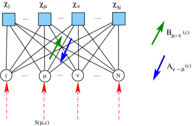
Figure 4: SCAP factor graph and direction of sent messages. Variables are represented by circles, constraints by squares.

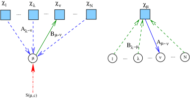
Figure 5: Pictorial representation of messages flow.

The set of equations of $A$ and $R$ can be solved iteratively via the BP algorithm. The case in which one is interested not in the whole form of the posterior probability function, but only in retaining information about the most probable exemplar chosen by each data point, can be seen to be equivalent to taking the $\beta\to\infty$ limit where availabilities $a$ and responsibilities $r$ are introduced in the following way:

$$A(\mu,\nu) = e^{\beta a(\mu,\nu)}e^{\beta{\hat{a}}_{\nu\to\mu}}$$ (20)

$${\hat{A}}_{\nu\to\mu} = e^{\beta{\hat{a}}_{\nu\to\mu}}$$ (21)

$$R(\mu,\nu) = e^{\beta r(\mu,\nu)+\beta max_{c:c\neq\nu}\{r_{\mu\to\nu}(c:c\neq\nu)\}}$$ (22)

$$B_{\mu\to\nu}(c:c\neq\nu) = e^{\beta r_{\mu\to\nu}(c:c\neq\nu)}$$ (23)

and treating the exponential scaling in a regime where prior similarities between data points $S$ are of the same order of magnitude of the valued of $a$ and $r$. The rescaling of responsibilities can be freely done as it does not change the number of independent variables. From the last definitions one is led to equations

$$A(\mu,\nu) = \frac{1}{1+(N-1)e^{-\beta a(\mu,\nu)}}$$ (24)

$$R(\mu,\nu) \sim \frac{1}{1+e^{-\beta r(\mu,\nu)}}$$ (25)

where the last relation already assumes a large-$\beta$ limit with non-degeneracy of the most probable value of the cavity probabilities. This hypothesis is equivalent to having non-degenerate choices of exemplars for all data points, i.e., to the existence of a single optimal clustering identified via the SCAP algorithm as the unique ground state of the system energy (3). This is a sensible assumption, but it is not always satisfied in interesting cases. Studying the degenerate number and behavior of clustering choices is another crucial question that is only partially answered by the introduction of the relaxation parameter $p$ and will be the subject of further work beyond this paper. In the large $\beta$ regime, in order to work with quantities all with the same scaling, it is useful to define

$$p=e^{-\beta{\tilde{p}}}$$ (26)

and consider ${\tilde{p}}$, $a$ and $r$ fixed varying $\beta$. Equating Eqs. (24) and (25) with Eqs. (17) and (19) respectively, and extracting the leading terms in the large $\beta$ limit assuming no degeneracy, the following equations are found, using Eq. (26):

$$r(\mu,\nu) = S(\mu,\nu)-{\max}_{\lambda\neq\nu}\big{[}S(\mu,\lambda)+a(\mu,\lambda)\big{]}$$

$$r(\mu,\mu) = S(\mu,\mu)-{\max}_{\lambda\neq\mu}\big{[}S(\mu,\lambda)+a(\mu,\lambda)\big{]}$$ (27)

$$a(\mu,\nu) = {\min}\Big{[}0,{\max}(-{\tilde{p}},{\min}(0,\ r(\nu,\nu)))+\sum_{\lambda\neq\mu}{\max}(0,\ r(\lambda,\nu)\Big{]}$$

$$a(\mu,\mu) = {\min}\Big{[}{\tilde{p}},\ \sum_{\lambda\neq\mu}{\max}\{0,r(\lambda,\mu)\}\Big{]}\ .$$

Making another change of variables redefining the self-responsibilities as

$$r^{\prime}(\mu,\mu)={\max}\big{[}-{\tilde{p}},r(\mu,\mu)\big{]}-{\max}_{\mu}\{r(\mu,\mu)\}\to r(\mu,\mu)$$ (28)

we get, in terms of the rescaled quantities,

$${\max}(-{\tilde{p}},{\min}(0,\ r(\mu,\mu)))=r(\mu,\mu)$$ (29)

leading to SCAP equations (5) . After convergence, marginals can be written Yedidia et al., (2005); Frey et al., (2007) as

$$P_{\mu}(c) \sim P^{BP}_{\mu}(c)\propto\prod_{\lambda}A_{\lambda\to\mu}(c)\exp(\beta S(\mu,c))$$ (30)

$$\propto R(\mu,c)A(\mu,c)\propto e^{\beta(a(\mu,c)+r(\mu,c))}$$

In the $\beta\to\infty$ limit, one can write equation  (6).

V Discussion

Affinity Propagation is a new powerful tool for unsupervised clustering. It has many very strong points. First it is very efficient, convergence to the final clustering is very fast, the latter appears to be independent on the initialization of messages. Second, due to its hard constraints AP identifies exemplars which are prototypical data points representing a whole cluster.

This last point is, however, also a first limitation of the original AP algorithm. If clusters cannot be well-represented by a single cluster exemplar, AP has to fail. The hard constraint renders the algorithm greedy, and small fluctuations in the similarity measure may trigger avalanches in the exemplar choice leading to different clusterings for only slightly modified model parameters.

We have introduced a soft-constraint version of affinity propagation which is able to cure a part of these problems without loosing the efficiency of the original AP:

• By relaxing the hard constraint on clusters exemplars, we could introduce a parameter ($\tilde{p}$) controlling the algorithm greediness. $\tilde{p}$ is a better tuning parameter than $\sigma$ (it is more informative and leads to more robust and stable clustering) and it is easier to interpret the statistical meaning of its tuning process.
  

• Clusters are more robust than in the original formulation of the algorithm. Moreover, even though a second a priori free-parameter is introduced, the overall dependence of the algorithm on free parameters is reduced, and an optimal tuning strategy naturally emerges.
  

• The cluster structure can be efficiently probed. This concerns the internal structure of the clusters since SCAP is able to identify central and peripherical nodes of each clusters, as well as the hierarchical organization leading to a process of cluster merging if cluster number is reduced by looking to less fine structures.
  

• In the case of high-dimensional data, the relation between data points and their exemplars can be used to extract a sparse cluster signature. In the case of brain tumors, we have found that 20-40 genes per cluster are sufficient to reproduce almost the same clustering as found using all genes.
  

We conclude that SCAP is more efficient than AP in particular in the case of noisy, irregularly organized data - and thus in biological applications concerning microarray data. The computational efficiency of SCAP allows there to treat also very large data sets.

References

- Frey et al., (2007) Frey, J.F. and Dueck, D. (2007) Clustering by Passing Messages Between Data Points, Science 315, 972-976.
- Frey et al., (2005) Frey, J.F. and Dueck, D. (2007) Mixture Modeling by Affinity Propagation, freely available at books.nips.cc/papers/files/nips18/NIPS2005_0799.pdf
- Jain et al., (1999) Jain, A.K., Murty, M.N., and Flynn, P.J. (1999) Data Clustering: A Review, ACM Computing Surveys, 31, 264-323.
- MacQueen, (1967) MacQueen,J., Proc. Fifth Berkeley Symp. on Mathematical Statistics and Probability, L. Le Cam, J. Neyman, Ed. (Univ. of California Press 1967), 281.
- Shi et al., (2000) Shi, J., Malik, J., (2000) IEEE Trans. Pattern Anal. Mach. Intell. 22, 888.
- Blatt et al., (1996) Blatt, M. , Wiseman, S. and Domany, E. (1996) Super-paramagnetic clustering of data, Physical Review Letters,76, 3251.
- Shental et al, (2003) Shental, N., Zomet, A., Hertz,T. and Weiss,Y. (2003) Pairwise Clustering and Graphical Models, 17th Int. Conf. on Neural Information Processing Systems - NIPS, Vancouver, Canada, December 2003.
- Duda et al., (1973) Duda, R. O. and Hart, P. E., Pattern Classification and Scene analysis (Wiley, NEw York 1973).
- Yedidia et al., (2005) Yedidia, J.S., Freeman, W.F., and Weiss, Y. (2005) Belief Propagation and Generalizations, IEEE Trans. Inform. Theory 51, 2282.
- Kschischang et al., (2001) F. R. Kschischang, B. J. Frey, H.-A. Loeliger, (2001) Factor Graphs and the Sum-Product Algorithm, IEEE Trans. Inform. Theory 47, 1.
- Pomeroy et al. (2002) Pomeroy, S., Tamayo, P., Gaasenbeek, M., Sturla, L., Angelo, M., McLaughlin, M., Kim, J., Goumnerova, L., Black, P., Lau, C. et al. (2002). Prediction of Central Nervous System Embryonal Tumor Outcome Based on Gene Expression. Nature 415, 436-442.
- Dettling (2004) Dettling, M. (2004), BagBoosting for Tumor Classification with Gene Expression Data, Bioinformatics 20, 3583-3593.
- Alizadeh et al. (2000) Alizadeh, A et al. (2000) Distinct types of diffuse large B-Cell-Lymphoma Identified by Gene Expression Profiling, Nature 403, 503-511.
- Kahn et al. (2001) Khan, J. et al. (2001) Classification and Diagnostic Prediction of Cancer Using Gene Expression Profiling and Artificial Neural Networks. Nature Medicine 6, 673-679.
- Golub et al. (1999) Golub, T. et al. (1999) Molecular Classification of Cancer: Class Discovery and Class Prediction by Gene Expression Monitoring. Science 286, 531-537.
- Braunstein and Zecchina (2006) Braunstein, A., Zecchina, R. (2006) Learning by Message passing in Networks of Discrete Synapses Phys Rev. Lett. 96 030201.
- Mézard et al. (2002) Mézard, M., Parisi, G., Zecchina, R. (2002) Analytic and Algorithmic Solution of Random Satisfiability Problems, Science 297, 812.
- Hartmann et al. (2005) Hartmann, A.K., Weigt, M. (2005) Phase Transitions in Combinatorial Optimization Problems (Wiley-VCH, Berlin 2005).
- Kabashima (2003) Kabashima, Y. (2003) A CDMA multiuser detection algorithm on the basis of belief propagation, J. Phys. A 36, 11111-11121.