Predicting and Understanding Order of Heteroepitaxial Quantum Dots.

Abstract

Heteroepitaxial self-assembled quantum dots (SAQDs) will allow breakthroughs in electronics and optoelectronics. SAQDs are a result of Stranski-Krastanow growth whereby a growing planar film becomes unstable after an initial wetting layer is formed. Common systems are Ge_xSi_1-x/Si and In_xGa_1-xAs/GaAs. For applications, SAQD arrays need to be ordered. The role of crystal anisotropy, random initial conditions and thermal fluctuations in influencing SAQD order during early stages of SAQD formation is studied through a simple stochastic model of surface diffusion. Surface diffusion is analyzed through a linear and perturbatively nonlinear analysis. The role of crystal anisotropy in enhancing SAQD order is elucidated. It is also found that SAQD order is enhanced when the deposited film is allowed to evolve at heights near the critical wetting surface height that marks the onset of non-planar film growth.

Pennsylvania State University, Department of Engineering Science and Mechanics, University Park, PA 16802

1 Introduction

Heteroepitaxial self-assembled quantum dots (SAQDs) represent an important step in the advancement of semiconductor fabrication at the nanoscale that will allow breakthroughs in optoelectronics and electronics.[1, 2, 3, 4, 5, 6, 7, 8, 9, 10, 11, 12] SAQDs are the result of a transition from 2D growth to 3D growth in strained epitaxial films such as $\mbox{Si}_{x}$$\mbox{Ge}_{1-x}$/Si and $\mbox{In}_{x}\mbox{Ga}_{1-x}\mbox{As}$/GaAs. This process is known as Stranski-Krastanow growth or Volmer-Webber growth.[13, 1, 14, 15]. In applications, order of SAQDs is a key factor. There are two types of order, spatial and size. Spatial order refers to the regularity of SAQD dot placement, and it is necessary for nano-circuitry applications. Size order refers to the uniformity of SAQD size which determines the voltage and/or energy level quantization of SAQDs. It is reasonable to expect that these type of order are linked, and it is important to understand the factors that determine SAQD order. Further understanding should help in the design and simulation of both spontaneous “bottom up” self-assembly and directed or guided self-assembly to enhance SAQD order. [16, 17, 18, 19, 20, 21, 22, 23] Order prediction inherently involves the modeling of stochastic processes. Recently, SAQD order has been modeled using a deterministic model with stochastic initial conditions in the linear approximation.[24, 25] This model was based on previous nucleationless models of SAQD formation.[26, 27, 28, 29] Here, this method of modeling SAQD order is improved by incorporating stochastic thermal fluctuations in the surface diffusion. Thus, the previously deterministic governing equations become stochastic. The final order predictions are qualitatively the same as for the previous linear model, but they are quantitatively different. Additionally, preliminary non-linear modeling results are presented. One non-linear model approximates a 1D surface, but incorporates the stochastic thermal fluctuations. The second non-linear model is of a 2D surface, but it is only implemented as a deterministic model at present.

In the previous work using a linear deterministic model with stochastic initial conditions[24, 25], it was found that peaks in the linear dispersion relation can be used to predict and explain order. It was also found that only anisotropic models give rise to dispersion relations with discrete peaks, thus explaining why elastic anisotropy contributes to SAQD order as previously reported.[30, 28, 31, 32] The dispersion relation was then used to generate a spectrum function in the linear approximation, and the spectrum function in turn could be used to define and predict two correlation lengths that grow as the square root of time. These correlation lengths were identified as the key quantities describing SAQD order. Using equations for these correlation lengths, it was found that growth of SAQDs with an average film height near the critical 2D-3D transition height might enhance order, although practical limitation of producing ordered arrays of SAQDs were also noted. Although the incorporation of a wetting potential is possibly controversial, it appears to produce the correct phenomenology, and it may possibly be a mathematical surrogate for more complicated processes such as stabilization by intermixing.[33] See refs.[34, 27, 29, 28, 26, 25] for further discussion. In ref.[25], it was also shown that the modeling/order prediction method could easily be applied to a large class of models, but the simplest model that produced Stranski-Krastanow growth was used as an example. Additionally, various mathematical issues such as convergence and precise definitions of the correlation functions as either spatial averages or ensemble averages was treated. Readers interested in these more technical details are referred to ref.[25].

The new result presented here is mainly the mentioned incorporation of thermal fluctuation to seed quantum dot formation, as opposed to the somewhat artificial assumption of a random roughness initial condition that is chosen more or less arbitrarily. One product of the present work is a formula to choose this initial roughness to give a nearly equivalent disordering effect as thermal fluctuations; however, a deterministic model will never be a true substitute for a stochastic one. The outcomes of the stochastic model are qualitatively similar to the previous deterministic model, but quantitatively distinct. In addition to the stochastic linear model of SAQD order, preliminary results of non-linear models are presented. These models appear to corroborate the linear model predictions but also give a more complete picture of the time evolution of SAQD order. The current model predicts that order will be fairly poor under most growth conditions. This seems to be in agreement with most experiments, for example refs.[35, 36, 14, 37, 38]. The basic phenomenology appears to be more or less in agreement with observations; however, more quantitative reporting of experimentally observed order would facilitate future comparisons.

The rest of this article is organized as follows. Section 2 presents the stochastic governing equations and physical causes of SAQD formation. Section 3 presents the linearization of the model presented in Sec. 2 along with the extraction of order predictions and application to growth near the critical film height using parameters appropriate to Ge/Si SAQDs. Section 4 presents preliminary non-linear modeling results. Section 5 presents the conclusion. Finally, Appendix A presents the derivation of the time evolution equation of the spectrum function.

2 Physical Model

The formation and growth of SAQDs is modeled in a fashion similar to refs.[26, 28, 27, 39, 18]. The film surface is described by the film height as a function of the lateral position, $0pt(\mathbf{x})$. The film height evolves via surface diffusion that is driven by a diffusion potential, $\mu(\mathbf{x})$. The film surface grows with a velocity normal to its surface that is given by

$$v_{n}(\mathbf{x}) = n_{z}(\mathbf{x})\frac{\partial 0pt(\mathbf{x)}}{\partial t}$$ (1)

$$= \boldsymbol{\nabla}_{s}\cdot\left[\mathcal{D}\boldsymbol{\nabla}_{s}\mu(\mathbf{x})+\sqrt{2\Omega\mathcal{D}k_{b}T}\boldsymbol{\eta}(\mathbf{x},t)\right]\dots$$

$$\dots+n_{z}(\mathbf{x})Q,$$

where $\mathcal{D}$ is the surface diffusivity; $n_{z}(\mathbf{x})$ is the $z-$component of the surface normal vector, $\hat{n}(\mathbf{x})$; $\boldsymbol{\nabla}_{S}$ is the surface gradient; $\boldsymbol{\nabla}_{S}\cdot$ is the surface divergence; $Q$ is the flux of new material onto the surface; and $\sqrt{2\Omega\mathcal{D}k_{b}T}\boldsymbol{\eta}(\mathbf{x},t)$ is the fluctuation of the surface diffusion. Note that the surface diffusivity is assumed to be a scalar; thus, it is isotropic. A limited discussion of diffusional anisotropy appears in ref.[25], and full development is in progress. The surface diffusion fluctuation is chosen to give a steady state that is consistent with the Gibbs distribution for a quadratic potential.[40] In ref. [40], there is a slope-dependent intensity factor, but here that factor is neglected for simplicity and because it has no effect to linear order. $\boldsymbol{\eta}(\mathbf{x},t)$ is a time fluctuating white noise (or the derivative of a Brownian process)[41, 42] so that it has zero mean $\left\langle\boldsymbol{\eta}(\mathbf{x},t)\right\rangle=0$, where $\left\langle\dots\right\rangle$ denotes the ensemble average, and it has a sharply peaked correlation function, $\left\langle\boldsymbol{\eta}(\mathbf{x},t)\boldsymbol{\eta}(\mathbf{x}^{\prime},t^{\prime})\right\rangle=\tilde{\mathbf{I}}\delta^{2}(\mathbf{x}-\mathbf{x}^{\prime})\delta(t-t^{\prime}).$ $\tilde{\mathbf{I}}$ is the rank 2 identity matrix, and $\delta(x)$ is the Dirac Delta function. Eq. 1 is interpreted as an Îto stochastic differential equation.

The diffusion potential is derived from the total free energy. The details of the derivation are covered in ref.[25], and only the most important points are reviewed here. The total free energy is assumed to have two parts, elastic energy and a term that is a combined surface energy and substrate wetting energy $\mathcal{F}=\mathcal{F}_{\text{elast.}}+\mathcal{F}_{sw}$. The second part $\mathcal{F}_{sw}$ is an integral over the horizontal coordinate $\mathbf{x}$ of an areal energy density,

$$\mathcal{F}_{sw}=\int_{\mathbf{x}-\text{plane}}d^{2}\mathbf{x}\,F_{sw}\left(0pt(\mathbf{x}),\boldsymbol{\nabla}0pt(\mathbf{x})\right).$$

The areal energy density, $F_{sw}$, is in turn a function of the film height, $0pt(\mathbf{x})$ and the film height gradient, $\boldsymbol{\nabla}0pt(\mathbf{x})$. From this total free energy, one can find the diffusion potential $\mu(\mathbf{x})$ by taking the variational derivative with respect to film height and multiplying by the atomic volume, $\Omega$,

$$\mu(\mathbf{x}) = \Omega\left[\omega(\mathbf{x})+F_{sw}^{\left(10\right)}(\mathbf{x})-\boldsymbol{\nabla}\cdot\mathbf{F}_{sw}^{\left(01\right)}(\mathbf{x})\right].$$ (2)

$\omega(\mathbf{x})$ is the elastic energy density at the film surface. $F_{sw}^{(mn)}$ indicates the $m^{\text{th}}$ derivative with respect to $0pt$ and the $n^{\text{th}}$ derivative with respect to $\boldsymbol{\nabla}0pt$. $F_{sw}^{\left(10\right)}(\mathbf{x})=\partial_{0pt(\mathbf{x})}F_{sw}\left(0pt(\mathbf{x}),\boldsymbol{\nabla}0pt(\mathbf{x})\right)$ and each vector component of $\mathbf{F}_{sw}^{\left(01\right)}(\mathbf{x})$ is $\left[\mathbf{F}_{sw}^{\left(01\right)}(\mathbf{x})\right]_{i}=\partial_{\left[\boldsymbol{\nabla}0pt(\mathbf{x})\right]_{i}}F_{sw}\left(0pt(\mathbf{x}),\boldsymbol{\nabla}0pt(\mathbf{x})\right)$. This diffusion potential (Eq. 2) is a general form for any surface diffusion model that incorporates the non-local elastic energy density and a local areal energy density such as a surface energy (even one with orientation dependence/faceting[27]) and a wetting energy.[34, 27, 29, 28] In refs.[24, 25] a simple model is analyzed that includes elastic anisotropy, a constant surface energy density, $\gamma$, and a substrate wetting energy density, $W(0pt)$. For this simple model, $F_{sw}=\left[1+\left(\boldsymbol{\nabla}0pt(\mathbf{x})\right)^{2}\right]^{1/2}\gamma+W\left(0pt(\mathbf{x})\right)$, and the resulting diffusion potential is

$$\mu(\mathbf{x})=\Omega\left[\omega(\mathbf{x})-\gamma\kappa(\mathbf{x})+W^{\prime}(0pt(\mathbf{x}))\right],$$ (3)

where $\kappa(\mathbf{x})$ is the total curvature, and $W^{\prime}(0pt)$ is just the derivative of the wetting potential. A more extensive discussion of different possibilities for $F_{sw}$ is discussed in ref.[25].

3 Linear Stochastic Model

Stochastic terms that fluctuate in time lead to stochastic differential equation that are often difficult so solve with either analytic techniques or numerical simulation. [42, 41] Linear stochastic differential equations, however, are much easier to solve. In fact, their solution is not very different from the solution of linear deterministic (or ordinary) differential equations with stochastic initial conditions. The linear model is naturally more approximate than the non-linear model, but it represents an important first step, and its solution can facilitate the development and interpretation of non-linear models.

To model the development of SAQD order, the growth dynamics are linearized producing a linear dispersion relation (Sec. 3.1). Then, the spectrum function is calculated based on the governing linear equations and the dispersion relation (Sec. 3.2). The expression for the spectrum function is then applied to the simple diffusion potential (Eq. 3) for a (100) surface of a cubic crystal (Sec. 3.3). Application of this method generally (to other surfaces or crystals) is outlined in ref.[25]. In this part of the calculation, crystal anisotropy can play an important role in the diffusion dynamics and development of SAQD order.[24, 25, 43, 28] For simplicity, it is assumed that only elasticity has a strong anisotropic effect. A more detailed analysis of other anisotropic effects can be very cumbersome.[25] Using the specific dispersion relation, formulas for the correlation lengths that quantify SAQD order and the real-space correlation function or derived. Finally, the correlation function and the correlation lengths are applied to a numerical example of Ge dots on a Si substrate. In this example, order predictions and dependence of order on average film height is compared with previous deterministic models.

3.1 Linearized Model

Figure 1: Evolving film surface. Total height is average ($\bar{0pt})$ plus fluctuations $h$.

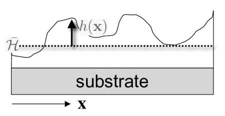
Eqs. 1 and 2 are linearized about the average film height (denoted $\bar{0pt}$) for the case of zero deposition rate ($Q=0$). Thus, the following analysis would correspond to a fast deposition and then an anneal. Other growth cases such as constant deposition rate can be analyzed in a similar fashion, but they are beyond the scope of the present work. Following refs.[44, 29], the total film height is the average film height plus small fluctuations (Fig. 1),

$$0pt(\mathbf{x},t)=\bar{0pt}+h(\mathbf{x},t).$$

Due to translational invariance of the governing equations, the Fourier components of $h(\mathbf{x},t)$ evolve independently in the linear model. Also, the non-local nature of the elastic energy makes calculations using Fourier components (spectral methods) easier than using $h(\mathbf{x},t)$. Fourier transforms use the convention, $f(\mathbf{x})=\int d^{2}\mathbf{k}\,e^{i\mathbf{k}\cdot\mathbf{x}}f_{\mathbf{k}}$ and $f_{\mathbf{k}}=(2\pi)^{-2}\int d^{2}\mathbf{x}\,e^{-i\mathbf{k}\cdot\mathbf{x}}f(\mathbf{x})$. $h_{\mathbf{k}}$ is the Fourier transform of $h(\mathbf{x})$, where $\mathbf{k}$ is the corresponding wave vector.

The linearized diffusion potential is calculated following ref.[25]. Linearizing the surface-wetting part of the diffusion potential, Eq. 2 and taking the Fourier transform, one gets[24]

$$\mu_{sw,\text{lin},\mathbf{k}}=\Omega\left(F_{sw}^{(20)}+\mathbf{k}\cdot\tilde{\mathbf{F}}_{sw}^{(02)}\cdot\mathbf{k}\right)h_{\mathbf{k}},$$

where the $F_{sw}^{(mn)}$ terms are the derivatives of $F_{sw}(0pt,\boldsymbol{\nabla}0pt)$, evaluated for a perfectly flat surface of height $\bar{0pt}$. They are constants in the following analysis because they depend only on the average film height $0pt$. The first superscript indicates the $m^{\text{th}}$ derivative of $F_{sw}$ with respect to $0pt$. The second index indicates the $n^{\text{th}}$ derivative with respect to $\boldsymbol{\nabla}0pt$. Evaluated for a perfectly flat surface of height $\bar{0pt}$, $F_{sw}^{\left(mn\right)}=\left.\partial_{0pt}^{m}\partial_{\boldsymbol{\nabla}0pt}^{n}F_{sw}\left(0pt,\boldsymbol{\nabla}0pt\right)\right|_{0pt=\bar{0pt},\,\boldsymbol{\nabla}0pt=\mathbf{0}}.$ The elastic energy density at the film surface is calculated as in refs.[25, 45, 46], where the bimaterial (film + substrate) is approximated as an elastically homogeneous material to simplify calculations. The resulting elastic energy density to linear order is $\omega_{\text{lin},\mathbf{k}}=-\mathcal{E}_{\theta_{\mathbf{k}}}kh_{\mathbf{k}}$ so that the elastic energy is proportional to the wavenumber $k=\left\|\mathbf{k}\right\|$ and the Fourier component $h_{\mathbf{k}}$, and it has a prefactor that depends on the wave vector direction, $\theta_{\mathbf{k}}$. Thus, the total linearized diffusion potential in reciprocal space is

$$\mu_{\text{lin},\mathbf{k}}=\Omega\left(-\mathcal{E}_{\theta_{\mathbf{k}}}k+F_{sw}^{(20)}+\mathbf{k}\cdot\tilde{\mathbf{F}}_{sw}^{(02)}\cdot\mathbf{k}\right)h_{\mathbf{k}}.$$ (4)

Linearizing the dynamic evolution, Eq. 1, and plugging in $Q=0$ and $\mu_{\text{lin},\mathbf{k}}$,

$$\partial_{t}h_{\mathbf{k}}(t) = \sigma_{\mathbf{k}}h_{\mathbf{k}}(t)+\sqrt{2\Omega\mathcal{D}k_{b}T}\left[i\mathbf{k}\cdot\boldsymbol{\eta}_{\mathbf{k}}(t)\right];$$ (5)

$$\sigma_{\mathbf{k}} = -k^{2}\mathcal{D}\Omega\left(-\mathcal{E}_{\theta_{\mathbf{k}}}k+F_{sw}^{(20)}+\mathbf{k}\cdot\tilde{\mathbf{F}}_{sw}^{(02)}\cdot\mathbf{k}\right),$$ (6)

where $\boldsymbol{\eta}_{\mathbf{k}}(t)$ is the Fourier transform of $\boldsymbol{\eta}(\mathbf{x},t)$. It has zero ensemble mean, $\left\langle\boldsymbol{\eta}_{\mathbf{k}}(t)\right\rangle=0$), and a sharply peaked two-point correlation function, $\left\langle\boldsymbol{\eta}_{\mathbf{k}}(t)\boldsymbol{\eta}_{\mathbf{k}^{\prime}}(t^{\prime})^{*}\right\rangle=(2\pi)^{-2}\delta^{2}(\mathbf{k}-\mathbf{k}^{\prime})\delta(t-t^{\prime}).$ The growth rate of each Fourier component, $\sigma_{\mathbf{k}}$, is dubbed the dispersion relation.

3.2 Spectrum Function

Eqs. 5 and 6 can be solved as a system of uncoupled linear stochastic ordinary differential equations with constant coefficients[42, 41] because the Fourier components, $h_{\mathbf{k}}$, evolve independently to linear order. One could assume that there are both stochastic initial conditions and thermal fluctuations; however, the purpose here is to analyze the impact of just the thermal fluctuations on order. It is assumed the film is perfectly flat at $t=0$, and that the instability is seeded by just the thermal noise. Thus, initially, $h_{\mathbf{k}}(0)=0$ for all $\mathbf{k}$, and to linear order, the ensemble average film height fluctuation remains zero for all time. However, the spectrum function, $C_{\mathbf{k}}(t)$ provides the lowest order non-trivial statistical description of film height fluctuations, and it is used to predict the order of SAQD arrays in a fashion similar to refs.[24, 25]. By taking the inverse Fourier transform of the spectrum function, one can predict the real-space correlation function (Sec. 3.3.1). A more complete picture of the interrelations between the spectrum function, the real-space correlation functions and other correlation functions is presented in ref.[25].

Taking the ensemble average of Eq. 5,

$$\partial_{t}\left\langle h_{\mathbf{k}}(t)\right\rangle=\sigma_{\mathbf{k}}\left\langle h_{\mathbf{k}}(t)\right\rangle+\sqrt{2\Omega\mathcal{D}k_{b}T}\left[i\mathbf{k}\cdot\left\langle\boldsymbol{\eta}_{\mathbf{k}}(t)\right\rangle\right].$$

The surface diffusion thermal fluctuation is mean-zero (Sec. 3.1), and the initial surface height fluctuation is mean-zero,$\left\langle h_{\mathbf{k}}(0)\right\rangle=0$; thus, $\left\langle h_{\mathbf{k}}(t)\right\rangle=0$ for all time.

Starting from the linearized governing equation and initial conditions, an evolution equation for the spectrum function can be derived that is both linear and deterministic (Appendix A),

$$\partial_{t}C_{\mathbf{k}}(t)=2\sigma_{\mathbf{k}}C_{\mathbf{k}}(t)+\frac{k^{2}}{(2\pi)^{2}}\left(2\Omega\mathcal{D}k_{b}T\right).$$ (7)

Using the initial condition that $C_{\mathbf{k}}(0)=0$,

$$C_{\mathbf{k}}(t)=\frac{\mathcal{D}\Omega k_{b}T}{(2\pi)^{2}\sigma_{\mathbf{k}}}k^{2}\left(e^{{2\sigma}_{\mathbf{k}}t}-1\right).$$ (8)

The spectrum function $C_{\mathbf{k}}(t)$ is the average value one would expect if one extracts from a simulation or experiment the film height power spectrum, $(2\pi)^{2}\left|h_{\mathbf{k}}(t)\right|^{2}/Area\approx C_{\mathbf{k}}(t)$. [25]

3.3 Application to (100) surfaces

The spectrum function time dependence, Eq. 8, is now applied to a (100) surfaces of cubic crystals using the simple diffusion potential, Eq. 3. Anisotropy plays an important role in order development, and for simplicity only elastic anisotropy is included. From this analysis, the two correlation lengths are found, and then the correlation function. Finally, a numerical example of Ge dots on a Si substrate is presented. The dependence of order on film height is investigated and compared and contrasted with the similar dependence from the previous deterministic model.[25]

3.3.1 Spectrum and Correlation function

If $\sigma_{\mathbf{k}}$ is peaked at wave vectors, $\mathbf{k}_{n}$, corresponding to some reciprocal lattice vectors, then a quasiperiodic arrangement of SAQDs can form during the initial stages of growth.[24, 25] This quasiperiodicity is demonstrated by applying the linearized simple diffusion potential, Eq. 3, along with elastic anisotropy $\omega(\mathbf{x})$ to Ge deposited on Si with a (100) substrate surface. For a (100) surface of a crystal with cubic symmetry, $\omega_{\text{lin},\mathbf{k}}=-\mathcal{E}_{0^{\circ}}\left(1-\epsilon_{A}\sin^{2}(2\theta_{\mathbf{k}})\right)kh_{\mathbf{k}}$ is a very good fit to a full elasticity calculation, where $\mathcal{E}_{0^{\circ}}$ is the elastic energy prefactor for $\theta_{\mathbf{k}}=0^{\circ}$, and $\epsilon_{A}=\left(\mathcal{E}_{0^{\circ}}-\mathcal{E}_{45^{\circ}}\right)/\mathcal{E}_{0^{\circ}}$ is an elastic anisotropy factor.[25] The resulting linear diffusion potential in reciprocal space is[25]

$$\mu_{\text{lin},\mathbf{k}}=\Omega\left[-\mathcal{E}_{0^{\circ}}\left(1-\epsilon_{A}\sin^{2}(2\theta_{\mathbf{k}})\right)k+\gamma k^{2}+W^{\prime\prime}(\bar{0pt})\right]h_{\mathbf{k}},$$

where $\gamma$ is the surface energy density, and $W^{\prime\prime}(0pt)$ is the second derivative of the wetting potential. One can see that this is a special case of Eq. 4.

The corresponding dispersion relation is

$$\sigma_{\mathbf{k}}=\mathcal{D}\Omega k^{2}\left[\mathcal{E}_{0^{\circ}}\left(1-\epsilon_{A}\sin^{2}(2\theta_{\mathbf{k}})\right)k-\gamma k^{2}-W^{\prime\prime}(\bar{0pt})\right],$$

assuming that diffusivity is isotropic as in refs.[25, 24].

From this dispersion relation, characteristic lengths and times can be found along with details of the early film evolution behavior. A characteristic wavenumber and time can be defined, $k_{c}=\mathcal{E}_{0^{\circ}}/\gamma$ and $t_{c}=\gamma^{3}(\mathcal{D}\Omega\mathcal{E}_{0^{\circ}}^{4})$. Also, the strength of the wetting term $W^{\prime\prime}(\bar{0pt})$ can be expressed as a dimensionless variable, $\beta=\gamma W^{\prime\prime}(\bar{0pt})/\mathcal{E}_{0^{\circ}}^{2}$. A detailed analysis[25, 24, 29, 27] shows that a large value of $W^{\prime\prime}(\bar{0pt})$ such that $\beta>1/4$ stabilizes a flat film to linear order in $h_{\mathbf{k}}$, while a small value of $W^{\prime\prime}(\bar{0pt})$ such that $\beta<1/4$ is insufficient to stabilize a flat film for all possible fluctuations, $h_{\mathbf{k}}$. For sufficiently small $\beta$, $\sigma_{\mathbf{k}}$ has 4 peaks along the four $\left\langle 100\right\rangle$ directions, corresponding to $\theta_{\mathbf{k}}=0^{\circ},\,90^{\circ},\,180^{\circ}$ and $270^{\circ}$ and $k=\alpha_{0}k_{c}$. $\alpha_{0}=\left(3+\sqrt{9-32\beta}\right)/8$ is a convenient dimensionless quantity. Thus, the four peaks occur at $\mathbf{k}_{1}=\alpha_{0}k_{c}\mathbf{i}$, $\mathbf{k}_{2}=\alpha_{0}k_{c}\mathbf{j}$, $\mathbf{k}_{3}=-\alpha_{0}k_{c}\mathbf{i}$ and $\mathbf{k}_{4}=-\alpha_{0}k_{c}\mathbf{j}$. Expanding $\sigma_{\mathbf{k}}$ in the vicinity of peak $n$,

$$\sigma_{\mathbf{k}}\approx\sigma_{0}-\frac{1}{2}\sigma_{\parallel}(k_{\parallel}-\alpha_{0}k_{c})^{2}-\frac{1}{2}\sigma_{\perp}k_{\perp}^{2},$$ (9)

where $k_{\parallel}$ is the component of $\mathbf{k}$ parallel to $\mathbf{k}_{n}$, and $k_{\perp}$ is the component of $\mathbf{k}$ perpendicular to $\mathbf{k}_{n}$. $\sigma_{0}=\frac{1}{4}t_{c}^{-1}\alpha_{0}^{2}\left(\alpha_{0}-2\beta\right)$, $\sigma_{\parallel}=t_{c}^{-1}k_{c}^{-2}\left(3\alpha_{0}-4\beta\right)$, and $\sigma_{\perp}=8\epsilon_{A}\alpha_{0}t_{c}^{-1}k_{c}^{-2}$.

Eq. 9 is used to find an approximate expression for the spectrum function $C_{\mathbf{k}}(t)$. $\sigma_{\mathbf{k}}$ appears inside an exponential; thus, for sufficiently large values $\sigma_{0}t$, the exponential term in the vicinity of the peaks will dominate over all other contributions to the spectrum function. Thus, $C_{\mathbf{k}}(t)$ will have the approximate form of four gaussians each centered around the four peak locations, $\mathbf{k}_{n}$. For sufficiently narrow gaussians, the prefactor can be approximated by its value at the peak. Thus,

$$C_{\mathbf{k}} (t)\approx \frac{\mathcal{D}\Omega k_{b}T}{(2\pi)^{2}\sigma_{0}}\left(\alpha_{0}k_{c}\right)^{2}e^{2\sigma_{0}t}\dots$$ (10)

$$\dots\times\sum_{n=1}^{4}e^{-\frac{1}{2}L_{\parallel}^{2}\left(k_{\parallel}-k_{0}\right)^{2}-\frac{1}{2}L_{\perp}^{2}k_{\perp}^{2}},$$

where

$$L_{\parallel}=\sqrt{2\sigma_{\parallel}t}=k_{c}^{-1}\sqrt{(6\alpha_{0}-8\beta)(t/t_{c})},$$ (11)

$$L_{\perp}=\sqrt{2\sigma_{\perp}t}=k_{c}^{-1}\sqrt{16\epsilon\alpha_{0}(t/t_{c})}.$$ (12)

Figure 2: (a) Film height and (b) spectrum function of the $\bar{0pt}=1.1$$0pt_{c}$ simulation discussed in Sec. 4.2 at the end time, $t=255t_{c}$. The drawn circle in (a) has a radius equal to $L_{\perp}$ calculated from the spectrum function (b).

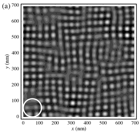
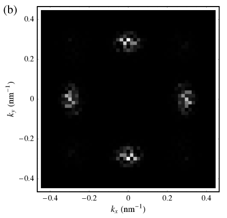
$L_{\parallel}$ and $L_{\perp}$ are the two correlation lengths that arose from models with deterministic evolution and stochastic initial conditions. They are measures of how spatially ordered an array of SAQDs is. The distance over which one can expect an array of SAQDs to appear periodic is about twice the smaller of the two correlation lengths, usually $L_{\perp}$.[24, 25] Fig. 2 shows an example of a film surface with the correlation length indicated. The approximate spectrum function, Eq. 10, is only valid when $\alpha_{0}k_{c}L_{\parallel}\gg 1$, and $\alpha_{0}k_{c}L_{\perp}\gg 1$. Of course, when this is not the case, order will be very poor. Thus, Eqs. 10–12 are useful for quantifying order when it is good, and they are able to indicate when order is poor.

The spectrum function, Eq. 10, is very similar to the spectrum function for the deterministic case with stochastic initial conditions characterized by a noise amplitude $\Delta^{2}$.[24, 25] If the noise amplitude is set to be

$$\Delta^{2}=\mathcal{D}\Omega k_{b}T\left(\alpha_{0}k_{c}\right)^{2}/\sigma_{0},$$

then the two cases are equivalent to linear order, when one performs these similar expansions. Often, one uses deterministic evolution equations with stochastic initial conditions as approximations to stochastic evolution equations. By performing a suitable linear analysis as done here, perhaps one can find an appropriate initial condition for such approximations. Note that $\Delta^{2}$ has dimensions of $\left[\text{length}\right]^{4}$, and the size of fluctuations in a discretization procedure changes with the discretization length scale. The spectral methods used here handle this problem fairly easily as one can coarse-grain a model by simply discarding fast oscillating noise components. A spatial discretization such as finite differencing or the finite element method makes quantitative implementation of white noise more complicated.

As with the deterministic model[24, 25], one can take the inverse Fourier transform of the spectrum function to obtain the real-space correlation function,

$$C(\boldsymbol{\Delta}\mathbf{x})=\frac{\mathcal{D}\Omega k_{b}T\left(\alpha_{0}k_{c}\right)^{2}}{\pi\sigma_{0}L_{\parallel}L_{\perp}}e^{2\sigma_{0}t}\dots$$ (13)

$$\dots\times\left[e^{-\frac{1}{2}\left(\Delta x^{2}/L_{\parallel}^{2}+\Delta y^{2}/L_{\perp}^{2}\right)}\cos(\alpha_{0}k_{c}\Delta x)\dots\right.$$

$$\dots+\left.e^{-\frac{1}{2}\left(\Delta x^{2}/L_{\perp}^{2}+\Delta y^{2}/L_{\parallel}^{2}\right)}\cos(\alpha_{0}k_{c}\Delta y)\right]$$

The correlation function, $C(\boldsymbol{\Delta}\mathbf{x})$, is a good predictor of the autocorrelation when the sampled or simulated area is very large.[25]

3.3.2 Numerical Example and film height dependence

In ref.[25], it was found that for reasonably soft wetting potentials, there can be some enhancement to spatial order when annealing takes place for films with heights, $\bar{0pt}$, that are only just above critical film height for unstable 3D growth. This finding was based on an assumption that the order that develops during the initial stages of growth is a meaningful order estimate. This assumption is justified to an extent by published numerical simulations[29, 28, 47, 48, 49] and is further justified by initial non-linear modeling results in Sec. 4. In ref.[25], the correlation lengths were found using parameters appropriate to Ge deposited on Si. A condition for the end of the linear evolution regime was taken to be when the r.m.s. film height fluctuation exceeded the atomic scale, the height of one monolayer. The r.m.s. height fluctuation is just $h_{\text{r.m.s.}}=\left[C\left(\mathbf{0}\right)\right]^{1/2}$, using Eq. 13. The time at which this condition was satisfied, $t_{\text{large}}$, was recorded, and the smaller correlation length, $L_{\perp}$ was calculated for this time. These predicted $t_{\text{large}}$ values and the number of correlated dots in a row were graphed vs. the dimensionless wetting potential strength for $\beta=0\dots 0.25$. It was found that the calculated time $t_{\text{large}}$ and the calculated correlation length diverge as $\beta\rightarrow 0.25$.

Figure 3: $t_{\text{large}}/t_{c}$ and $L_{\perp}/L_{0}$ vs. the dimensionless wetting parameter $\beta$ for Ge/Si at $T=600^{\circ}\text{C}$ as discussed in Sec. 3.3.2

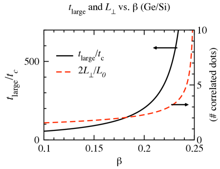
The same procedure is now followed for the present model for Ge on Si with temperature $T=600^{\circ}\text{ C}$. All values are the same as for the calculations in ref.[25]. The results are graphed in Fig. 3. When compared with the results from the deterministic model with stochastic initial conditions[25], one finds that the effect of thermal fluctuations in the surface diffusion are actually more disruptive to order than assuming an initial surface with atomic scale roughness. The qualitative trends are the same,however, and the divergence in correlation length as $\beta\rightarrow 0.25$ is observed. As discussed in ref.[25], one should take care interpreting this result, and there are of course practical limitations. The order enhancing effect of near critical growth has not been experimentally observed (or looked for), and there may be practical limitation to implementing near critical growth as a method to enhance order such as the requirement for precise deposition control.

4 Perturbatively Non-Linear Models

The order estimates presented in refs.[24, 25] and Sec. 3.3.2 are based on the order that develops before fluctuations become large. The significance of these calculations is based on the following observations:

1. Order increases during the linear stage of growth as $t^{1/2}$ (Eqs. 11 and 12).

2. Order does not increase forever. If it did, growing perfectly ordered arrays of dots would be trivial. Also, qualitative analysis of numerical simulations bears this out. [29, 28, 47, 48, 49]

It is, of course, worthwhile to extend the method of quantifying and predicting order to non-linear models. Non-linear stochastic modeling can be very cumbersome and difficult to implement, but some preliminary results are presented here. The same system as in Sec. 3.3.2 and ref.[25] is modeled here, and the same parameters are used.

4.1 1D Multiscale-Multitime Expansion

First, the results of a 1D non-linear model with stochastic evolution is presented. As a first attempt at non-linear modeling, two approximations are made. First, the elastic and surface energy parts are completely linearized. Second, the wetting potential, $W(0pt)$ is treated using a multiscale-multitime expansion. [29, 50] Full details of the model are omitted out of space considerations and because these are preliminary results.

Figure 4: Time dependence of number of correlated dots $L_{\text{cor}}/L_{0}$ vs. dimensionless time, $t/t_{c}$ for 1D stochastic film evolution (Sec. 4.1). Both linear model and multiscale expansion results are shown.

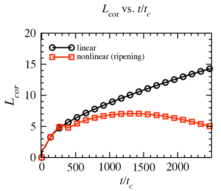
Based on ref.[27], the wetting potential is chosen to be $W(0pt)=2.314\times 10^{-6}/0pt\text{ erg/cm}^{2}$ with $0pt$in cm. This gives a critical film height of 4 monolayers $=1.132\text{ nm}$. The simulated film has an average film height of $\bar{0pt}=1.358\text{ nm}$ giving $\beta=0.1447$. The simulation cell size is $19.68\,\mu\text{m}$, large enough to hold 513 dots of average size $L_{0}=2\pi/k_{0}=38.4\text{ nm}$. The multiscale-multitime expansion uses an expansion in a scale variable $\epsilon$ to create a perturbation-like series. Additionally, fast oscillating Fourier components of $W(0pt)$ are discarded so that the natural length scale is the average size of a single dot, $L_{0}$ . To fourth order in $\epsilon$, one obtains a set of two coupled partial differential equations.[29, 50] These equations are solved using Stochastic Euler numerical integration[41, 42] implemented with Mathematica.[51] Computational efficiency is greatly enhanced by the multiscale-multitime expansion, but of course, accuracy and fidelity to the original model is partially sacrificed. Correlation lengths are calculated from the peak widths of the spectrum function ($\Delta k$), using $L_{\text{cor}}=1/\Delta k$. The number of dots in a row that form a recognizably periodic structure is $\#dots=2L_{\text{cor}}/L_{0}$. The time evolution of this number is plotted for both the linear model and the stochastic simulation (Fig. 4). The linear model has a correlation length that grows indefinitely. The non-linear model has a correlation length that grows to a peak value and then shrinks. In this case, the onset of ripening ruins the SAQD order. The onset of ripening in this model corresponds to the “blow-up solution” in ref.[29]

4.2 2D non-linear deterministic model

Figure 5: Dimensionless correlation length vs. dimensionless time for 2D non-linear deterministic model with stochastic initial conditions. Results for two different average film height are reported, $\bar{0pt}=1.250pt_{c}$ and $\bar{0pt}=1.10pt_{c}$

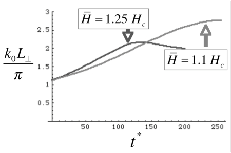
A similar result is obtained for a 2D deterministic non-linear model. This model treats the surface energy and wetting energy in full non-linear fashion. The non-local elastic part is found to cubic order in the film height fluctuation in $h$ via a perturbation series. The stochastic initial conditions are sampled white noise with an initial atomic scale roughness, corresponding to $\Delta^{2}=0.0403\text{ nm}^{4}$.[25] The critical height for the 2D-to-3D-growth transition is $0pt_{c}=1.132\text{ nm}$. Two initial average film heights are used to investigate the trend predicted in Fig. 3, $\bar{0pt}=1.250pt_{c}=1.415\text{ nm}$ ($\beta=0.1280$) and $\bar{0pt}=1.10pt_{c}=1.245\text{ nm}$ ($\beta=0.1878$). The simulation cell size corresponds to 17 dots squared = 289 dots. The time evolution equations are solved using the native numerical differential equation solver in Mathematica.[51] The correlation lengths vs. dimensionless time are plotted for both cases in Fig. 5. In both cases, the correlation length increases early on while fluctuations are small, reaches a peak value and then decreases due to ripening. The peak value of the correlation length is greater for the second case with $\beta$ closer to the optimal value of $1/4$. The 2D non-linear deterministic model further substantiates the theory that order develops during the early growth stages and then is diminished during ripening. Furthermore, the trend predicted by the linear order model is it least qualitatively corroborated because growth near the critical threshold enhances the peak order of SAQDs according to the 2D non-linear model.

5 Conclusions

A linear stochastic model of SAQD order has been presented as an extension of a previous linear deterministic model of the order of epitaxial self-assembled quantum dots (SAQDs). In addition, some preliminary results from non-linear stochastic and non-linear deterministic models have been presented to substantiate the significance of, extend and clarify the linear models of SAQD order. The presented numerical examples were based on a very simple SAQD model, and there has been much advancement in SAQD growth modeling; however, the presented procedure should apply equally well to a wide variety of models with various phenomenological assumptions and help to augment them and quantitatively extract order predictions. The current stochastic model should be augmented in the future to reflect these advances. Some adaptation of the method ought to apply to attempts to engineer SAQD order as well, such as substrate patterning or growing multilayers of SAQDs. As with the previous deterministic model, two correlation lengths are found, longitudinal $L_{\parallel}$ and transverse $L_{\perp}$ . The transverse correlation length appears to be the most limiting, and thus should be used to estimate order. It is found that if a wetting potential is incorporated that is sufficiently soft, growth near the 2D-3D transition critical film height enhances SAQD order; however, this enhancement would require very precise experimental control to implement. Nevertheless, it demonstrates how the presented methods might apply to other attempts to optimize SAQD growth and could help engineer those processes. It was also found that the previous deterministic model can be made approximately equivalent to the present stochastic model by choosing the appropriate initial conditions. Preliminary non-linear modeling appears to corroborate these claims, at least qualitatively. A quantitative comparison is still needed. The method to extract SAQD order should help with phenomenological model development as the correlation lengths and possibly other statistical characterization should facilitate quantitative tuning of phenomenological models to experiments. The models presented here apply to the nucleationless mode of SAQD formation; however, the inclusion of thermal fluctuations in non-linear models should facilitate a conceptual and/or mathematical unification of models of SAQD thermal nucleation and the nucleationless mode.

Thanks to L. Fang for a critical reading of this manuscript.

Appendix A Derivation of Eq. 7

The two-point correlation function in reciprocal space is

$$C_{\mathbf{k}\mathbf{k}^{\prime}}(t)=\left\langle h_{\mathbf{k}}(t)h_{\mathbf{k}^{\prime}}(t)^{*}\right\rangle.$$

Note that at time $t=0$, $C_{\mathbf{k}\mathbf{k}^{\prime}}(0)=\left\langle h_{\mathbf{k}}(0)h_{\mathbf{k}^{\prime}}(0)^{*}\right\rangle=0$. The time evolution of $C_{\mathbf{k}\mathbf{k}}(t)$ can be found using the stochastic chain rule ($\hat{\text{I}}$to’s lemma) and then taking the ensemble average.[41, 42]

$$\partial_{t}C_{\mathbf{k}\mathbf{k}^{\prime}}(t) = \left(\sigma_{\mathbf{k}}+\sigma_{\mathbf{k}^{\prime}}\right)C_{\mathbf{k}\mathbf{k}^{\prime}}(t)\dots$$ (15)

$$\dots+\frac{\mathbf{k}\cdot\mathbf{k}^{\prime}}{(2\pi)^{2}}\left(2\Omega\mathcal{D}k_{b}T\right)\delta^{2}(\mathbf{k}-\mathbf{k}^{\prime}).$$

The thermal fluctuations only contribute if $\mathbf{k}=\mathbf{k}^{\prime}$. Since initially $C_{\mathbf{k}\mathbf{k}^{\prime}}(0)=0$, one can expect $C_{\mathbf{k}\mathbf{k}^{\prime}}(t)$ to be non-zero only if $\mathbf{k}=\mathbf{k}^{\prime}$. Thus, the two-point correlation function is determined completely by the ensemble averaged spectrum function, $C_{\mathbf{k}}(t)$ as in ref.[25],

$$C_{\mathbf{k}\mathbf{k}^{\prime}}(t)=C_{\mathbf{k}}(t)\delta^{2}(\mathbf{k}-\mathbf{k}^{\prime}).$$ (16)

This results is only strictly true for the linearized equation. From Eq. 15 the time evolution equation of the spectrum function is found by inspection to be Eq. 7.

References

- [1] D. Bimberg, M. Grundmann, and N. N. Ledentsov. Quantum Dot Heterostructures. John Wiley & Sons, (1999).
- [2] O. P. Pchelyakov, Yu. B. Bolkhovityanov, A. V. Dvurechenski, L. V. Sokolov, A. I. Nikiforov, A. I. Yakimov, and B. Voigtländer. Semiconductors, 34:122947, (2000).
- [3] M. Grundmann. Physica E, 5:167, (2000).
- [4] Pierre M. Petroff, Axel Lorke, and Atac Imamoglu. Phys. Today, page 46, (2001).
- [5] Hui-Yun Liu, Bo Xu, Yong-Qiang Wei, Ding Ding, Jia-Jun Qian, Qin Han, Ji-Ben Liang, and Zhan-Guo Wang. Appl. Phys. Lett., 79:2868, (2001).
- [6] F. Heinrichsdorff, M.H. Mao, N. Kirstaedter, A. Krost, D. Bimberg, A. O. Kosogov, and P. Werner. Appl. Phys. Lett., 71:22, (1997).
- [7] D. Bimberg, N.N. Ledentsov, and J.A. Lott. MRS Bull., 27:531, (2002).
- [8] N. N. Ledentsov. IEEE J. Sel. Top. Quant., 8:1015, (2002).
- [9] M Friesen, P Rugheimer, D. E. Savage, M. G. Lagally, D. W. van der Weide, R Joynt, and M. A. Eriksson. Phys. Rev. B, 67:121301 (R), (2003).
- [10] Yi-Chang Cheng, San-Te (Cing-Ming) Yang, Jyh-Neng Yang, Liann-Be Chang, and Li-Zen Hsieh. Opt. Eng., 42:11923, (2003).
- [11] R. Krebs, S. Deubert, J.P. Reithmaier, and A. Forchel. J. Cryst. Growth, 251:7427, (2003).
- [12] Hiroyuki Sakaki. J. Cryst. Growth, 251:9, (2003).
- [13] B. J. Spencer, P. W. Voorhees, and S. H. Davis. Phys. Rev. Lett., 67:3696, (1991).
- [14] Karl Brunner. Rep. Prog. Phys., 65:27, (2002).
- [15] L. B. Freund and S. Suresh. Thin Film Materials: Stress, Defect Formation and Surface Evolution, chapter 8. Cambridge University Press, (2003).
- [16] S. Yu Shiryaev, E. Verstlund Pedersen, F. Jensen, J. Wulff Petersen, J. Lundsgaard Hansen, and A. Nylandsted Larson. Thin Solid Films, 294:311, (1997).
- [17] C. Kumar and L. H. Friedman. J. Appl. Phys., in press.
- [18] Lawrence H. Friedman and Jian Xu. Appl. Phys. Lett., 88:093105, (2006).
- [19] S. Krishna, D. Zhu, J. Xu, and P. Bhattacharya. J. Appl. Phys., 86:6135, (1999).
- [20] R. Hull, J.L. Gray, M. Kammler, T. Vandervelde, T. Kobayashi, P. Kumar, T. Pernell, J.C. Bean, J.A. Floro, and F.M. Ross. Mat. Sci. Eng. B-Solid, 101:1, (2003).
- [21] O. Guise, Jr. J. T. Yates, J. Levy, J. Ahner, V. Vaithyanathan, and D. G. Schlom. Appl. Phys. Lett., 87:171902, (2005).
- [22] X. Niu, R. Vardavas, R. E. Caflisch, and C. Ratsch. Phys. Rev. B, 74:193403, (2006).
- [23] Z. M. Zhao, T. S. Yoon, W. Feng, B. Y. Li, J. H. Kim, J. Liu, O. Hulko, Y. H. Xie, H. M. Kim, K. B. Kim, H. J. Kim, K. L. Wang, C. Ratsch, R. Caflisch, D. Y. Ryu, and T. P. Russell. Thin Solid Films, 508:195, (2006).
- [24] Lawrence H. Friedman. Phys. Rev. B, 75:193302, 2007.
- [25] Lawrence H. Friedman. arxiv:0704.0067v1 [cond-mat.mtrl-sci].
- [26] B. J. Spencer, P. W. Voorhees, and S. H. Davis. J. Appl. Phys., 73:4955, (1993).
- [27] Y.W. Zhang, A.F. Bower, and P. Liu. Thin Solid Films, 424:9, (2003).
- [28] P. Liu, Y. W. Zhang, and C. Lu. Phys. Rev. B, 67:165414, (2003).
- [29] A. A. Golovin, S. H. Davis, and P. W. Voorhees. Phys. Rev. E, 68:056203, (2003).
- [30] V. Holy, G. Springholz, M. Pinczolits, and G. Bauer. Phys. Rev. Lett., 83:356, (1999).
- [31] P. Liu, Y. W. Zhang, and C. Lu. Phys. Rev. B, 68:195314, (2003).
- [32] G. Springholz, M. Pinczolits, V. Holy, S. Zerlauth, I. Vavra, and G. Bauer. Physica E, 9:149, (2001).
- [33] Y. H. Tu and J. Tersoff. Phys. Rev. Lett., 93:216101, (2004).
- [34] M. J. Beck, A. van de Walle, and M. Asta. Phys. Rev. B, 70:205337, (2004).
- [35] J. M. Baribeau, X. Wu, N. L. Rowell, and D. J. Lockwood. J. Phys.-Condens. Mat., 18:R139, (2006).
- [36] I. Berbezier, A. Ronda, F. Volpi, and A. Portavoce. Surf. Sci., 531:231, (2003).
- [37] H. J. Gao and W. D. Nix. Ann. Rev. Mater. Sci., 29:173, (1999).
- [38] J. R. R. Bortoleto, H. R. Gutierrez, M. A. Cotta, J. Bettini, L. P. Cardoso, and M. M. G. de Carvalho. Appl. Phys. Lett., 82:3523, (2003).
- [39] W. T. Tekalign and B. J. Spencer. J. Appl. Phys., 96:5505, (2004).
- [40] Rodolfo Cuerno and Mario Castro. In P. Neittaanmäki, T. Rossi, O. Pironneau, R. Owen, and M. Mikkola, editors, Proceedings of the 4th. European Congress on Computational Methods in Applied Sciences and Engineering (ECCOMAS 2004), Finland, (2004). Jyväskylä.
- [41] Thomas Mikosch. ementary Stochastic Calculus With Finance in View, volume 6 of Advanced Series on Statistical Science & Applied Probability. World Scientific Publishing Company, Singapore, (1998).
- [42] C. W. Gardiner. Handbook of Stochastic Methods for Physics Chemistry and the Natural Sciences. Springer, New York, 3rd edition, (2004).
- [43] P. Liu, Y. W. Zhang, and C. Lu. Surf. Sci., 526:375, (2003).
- [44] B. J. Spencer, S. H. Davis, and P. W. Voorhees. Phys. Rev. Lett., 47:9760, (1993).
- [45] Y. Obayashi and K. Shintani. J. Appl. Phys., 84:3141, (1998).
- [46] C. S. Ozkan, W. D. Nix, and H. J. Gao. J. Mater. Res., 14:3247, (1999).
- [47] P. Liu, Y. W. Zhang, and C. Lu. Phys. Rev. B, 68:035402, (2003).
- [48] Yu U. Wang, Yongmei M. Jin, and Armen G. Khachaturyan. Acta Mater., 52:81, (2004).
- [49] F. M. Ross, J. Tersoff, and R. M. Tromp. Phys. Rev. Lett., 80:984, (1998).
- [50] M. C. Cross and P. C. Hohenberg. Rev. Mod. Phys., 65:851, (1993).
- [51] Mathematica version 5.2 (http://www.wolfram.com/).