Fourier Synthesis Methods for Control of Inhomogeneous Quantum Systems

Abstract

Finding control laws (pulse sequences) that can compensate for dispersions in parameters which govern the evolution of a quantum system is an important problem in the fields of coherent spectroscopy, imaging, and quantum information processing. The use of composite pulse techniques for such tasks has a long and widely known history. In this paper, we introduce the method of Fourier synthesis control law design for compensating dispersions in quantum system dynamics. We focus on system models arising in NMR spectroscopy and NMR imaging applications.

I Introduction

Many applications in the control of quantum systems involve controlling a large ensemble using the same control signal [1, 2]. In many practical cases, the elements of the ensemble show dispersions or variations in the parameters which govern the dynamics of each individual system. For example, in magnetic resonance experiments, the spins in an ensemble may have large dispersions in their resonance frequencies (Larmor dispersion) or in the strength of the applied radio frequency fields (rf inhomogeneity) seen by each member of the ensemble. Another example is in the field of NMR imaging, where a dispersion is intentionally introduced in the form of a linear gradient [2], and then exploited to successfully image the material under study.

A canonical problem in the control of quantum ensembles is the design of rf fields (control laws) which can simultaneously steer a continuum of systems, characterized by the variation in the internal parameters governing the systems, from a given initial distribution to a desired final distribution. Such control laws are called compensating pulse sequences in the Nuclear Magnetic Resonance (NMR) literature. From the standpoint of mathematical control theory, the challenge is to simultaneously steer a continuum of systems between points of interest using the same control signal. Typical designs include excitation and inversion pulses in NMR spectroscopy and slice selective pulses in NMR imaging [2, 5, 6, 7, 8, 9, 10, 11, 12, 13, 14]. In many cases, one desires to find a control law that prepares the final state as some desired function of the parameters. A premier example is the design of slice selective pulse sequences in magnetic resonance imaging applications, where spins are excited or inverted depending upon their physical position in the sample under study [2, 3, 15, 16, 17, 18]. In fact, the design of such pulses is a fundamental requisite for almost all magnetic resonance imaging techniques. This paper introduces the new method of Fourier synthesis pulse sequence design for systems showing dispersions in the parameters governing their dynamics.

In this paper we focus on the Bloch equations with a linear one dimensional gradient, which arise in the context of NMR spectroscopy and NMR imaging applications.

$$\frac{d}{dt}\left[\begin{array}[]{c}M_{x}\\ M_{y}\\ M_{z}\end{array}\right]=\left[\begin{array}[]{ccc}0&-G(t)s&\epsilon u(t)\\ G(t)s&0&-\epsilon v(t)\\ -\epsilon u(t)&\epsilon v(t)&0\end{array}\right]\left[\begin{array}[]{c}M_{x}\\ M_{y}\\ M_{z}\end{array}\right]$$ (1)

Here, $M(s,\epsilon)=[M_{x}\ M_{y}\ M_{z}]^{T}$ is the state vector, $u(t)\in\Re$, $v(t)\in\Re$, and $G(t)\in\Re$ are controls and the parameters $s\in[0,1]$ and $\epsilon\in[1-\delta,1],\ \delta>0$ are dispersion parameters which will be explained subsequently. Without loss of generality, we will always normalize the initial state of the system (1) to have unit norm, so that the system evolves on the unit sphere in three dimensions (Bloch sphere). A useful way to think about the Bloch equations (1), is by imagining a two dimensional mesh of systems, each with a particular value of the pair $(s,\epsilon)$. We are permitted to apply a single set of controls $(u(t),v(t),G(t))$ to the entire mesh of systems, and the controls should prepare the final state of each system as a desired function of the parameters $(s,\epsilon)$ which govern the system dynamics.

From a physics perspective, the system (1) corresponds to an ensemble of noninteracting spin-$\frac{1}{2}$ in a static magnetic field $B_{0}$ along the $z$ axis and a transverse rf field $(A(t)\cos(\psi(t)),A(t)\sin(\psi(t)))$ in the $x$-$y$ plane. The state vector $[M_{x}\ M_{y}\ M_{z}]^{T}$ represents the coordinate of the unit vector in the direction of the net magnetization vector for the ensemble [4]. The controls $u(t)$ and $v(t)$ correspond to available rf fields we may apply to the ensemble of spins. The dispersion in the magnitude of the rf field applied to the sample is modeled by including a dispersion parameter $\epsilon$ such that $A(t)=\epsilon A_{0}(t)$ with $\epsilon\in[1-\delta,1],\ \delta>0$. Thus, the maximum amplitude for the rf field ($\epsilon=1$) corresponds to the maximum amplitude seen by any spin in the ensemble. Similarly, we consider a linear gradient $G(t)s$, where $G(t)$ may be thought of as a control, and $s$ represents the normalized spatial position of the spin system in the sample of interest. In (1), we work in units with the gyromagnetic ratio of the spins $\gamma=1$. In this paper we give new design methods which scale polynomially that can be used to design pulse sequences for (1) which prepare the final state of the system as a function of the parameters $s$ and $\epsilon$.

II Design Method for rf Inhomogeneity

Considering only the Bloch equations with rf inhomogeneity and no linear gradient ($G(t)=0$), we can rewrite (1) in terms of the generators of rotation in three dimensions as

$$\frac{d}{dt}\left[\begin{array}[]{c}M_{x}\\ M_{y}\\ M_{z}\end{array}\right]=\epsilon(u(t)\Omega_{y}+v(t)\Omega_{x})\left[\begin{array}[]{c}M_{x}\\ M_{y}\\ M_{z}\end{array}\right]$$ (2)

where

$$\Omega_{x} = \left[\begin{array}[]{ccc}0&0&0\\ 0&0&-1\\ 0&1&0\end{array}\right]$$ (6)

$$\Omega_{y} = \left[\begin{array}[]{ccc}0&0&1\\ 0&0&0\\ -1&0&0\end{array}\right]$$ (10)

$$\Omega_{z} = \left[\begin{array}[]{ccc}0&-1&0\\ 1&0&0\\ 0&0&0\end{array}\right]$$ (14)

We will come back to the full version of the Bloch equations (1) with both a linear gradient and rf inhomogeneity later in the paper. The problem is to design $u(t)\in\Re$ and $v(t)\in\Re$ to effect some desired evolution. We now show how to construct controls to give a rotation of angle $\phi(\epsilon)$ around the $x$ axis or the $y$ axis of the Bloch sphere. From these constructions, an arbitrary rotation on the Bloch sphere can be constructed using an Euler angle decomposition.

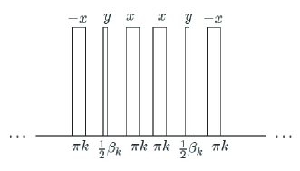
Figure 1: A schematic depiction of the pulse sequence element in (15). The pulse sequence element consists of six individual rotations which can be produced using the controls $u(t)$ and $v(t)$ as explained in the text.

II-A Rotation About $y$ axis

In a time interval $dt$, we can use the controls to generate rotations $\exp(\epsilon u_{0}dt\Omega_{y})$ and $\exp(\epsilon v_{0}dt\Omega_{x})$ where $u_{0}$ and $v_{0}$ are constants to be specified. Using this idea, consider generating the rotation

$$U_{k}=U_{1k}U_{2k}$$ (15)

with

$$U_{1k} = \exp(-\pi k\epsilon\Omega_{x})\exp(\frac{1}{2}\epsilon\beta_{k}\Omega_{y})\exp(\pi k\epsilon\Omega_{x})$$ (16)

$$U_{2k} = \exp(\pi k\epsilon\Omega_{x})\exp(\frac{1}{2}\epsilon\beta_{k}\Omega_{y})\exp(-\pi k\epsilon\Omega_{x})$$ (17)

using the controls $u$ and $v$. Using the relation

$$\exp(\alpha\Omega_{x})\exp(\beta\Omega_{y})\exp(-\alpha\Omega_{x})=$$

$$\exp(\beta(\cos(\alpha)\Omega_{y}+\sin(\alpha)\Omega_{z}))$$ (18)

the matrices $U_{1k}$ and $U_{2k}$ may be rewritten as

$$U_{1k} = \exp(\frac{1}{2}\epsilon\beta_{k}(\Omega_{y}\cos(\pi k\epsilon)-\Omega_{z}\sin(\pi k\epsilon)))$$ (19)

$$U_{2k} = \exp(\frac{1}{2}\epsilon\beta_{k}(\Omega_{y}\cos(\pi k\epsilon)+\Omega_{z}\sin(\pi k\epsilon)))$$ (20)

For small $\beta_{k}$, we can make the approximation

$$U_{1k}U_{2k}\approx\exp(\epsilon\beta_{k}\cos(\pi k\epsilon)\Omega_{y})$$ (21)

In (21), we have expanded the exponentials in $U_{1k}$ and $U_{2k}$ to first order, performed the multiplication called for in (15), and then rewritten the product as (21) keeping terms to first order. In the case when $\beta_{k}$ is too large for (21) to represent a good approximation, we should choose a threshold value $\beta_{0}$ such that (21) represents a good approximation and so that

$$\beta_{k}=n\beta_{0}$$ (22)

with $n$ an integer. Defining

$$U_{10} = \exp(\frac{1}{2}\epsilon\beta_{0}(\Omega_{y}\cos(\pi k\epsilon)-\Omega_{z}\sin(\pi k\epsilon)))$$ (23)

$$U_{20} = \exp(\frac{1}{2}\epsilon\beta_{0}(\Omega_{y}\cos(\pi k\epsilon)+\Omega_{z}\sin(\pi k\epsilon)))$$ (24)

we can apply the total propagator

$$[\ U_{10}U_{20}\ ]^{n}$$ (25)

$$\approx\left[\exp(\epsilon\beta_{0}\cos(\pi k\epsilon)\Omega_{y})\right]^{n}$$ (26)

$$=\exp(\epsilon\beta_{k}\cos(\pi k\epsilon)\Omega_{y})$$ (27)

where we used the approximation (21) in (26). More will be said about this approximation below.

If we then think about making the incremental rotation $U_{k}$ for many different values of $k$, we will get a net rotation

$$U=\prod_{k}\exp(\epsilon\beta_{k}\cos(\pi k\epsilon)\Omega_{y})$$ (28)

so long as we keep $\beta_{k}$ sufficiently small to justify the approximation (21). The total propagator $U$ for the Bloch equations can then be rewritten as

$$U=\exp(\epsilon\sum_{k}\beta_{k}\cos(\pi k\epsilon)\Omega_{y})$$ (29)

If we now choose the coefficients $\beta_{k}$ so that

$$\sum_{k}\beta_{k}\cos(\pi k\epsilon)\approx\frac{\phi(\epsilon)}{\epsilon}$$ (30)

then we will have constructed a pulse sequence to approximate a desired $\epsilon$ dependent rotation around the $y$ axis. Since $\epsilon$ is bounded away from the origin, $\phi(\epsilon)/\epsilon$ is everywhere finite, and we can approximate it with a Fourier Series.

II-A1 Remark About the Approximation

Here we consider the error introduced by the approximation (26). Define the error $E(Z,V)$ when a unitary matrix $V$ is implemented instead of a desired unitary matrix $Z$ by

$$E(Z,V)=\max_{x}\|(Z-V)x\|$$ (31)

With these identifications, in (25) we have

$$V = U_{10}U_{20}$$ (32)

$$= I+\frac{\beta_{k}}{n}\cos(\pi k\epsilon)\Omega_{y}+M_{1}(n)$$

and

$$Z = \exp(\beta_{0}\cos(\pi k\epsilon)\Omega_{y})$$ (33)

$$= I+\frac{\beta_{k}}{n}\cos(\pi k\epsilon)\Omega_{y}+M_{2}(n)$$

where $M_{1}(n)$ and $M_{2}(n)$ are matrices with finite entries and of maximum order $\frac{1}{n^{2}}$. Notice this implies that the difference $(Z-V)$ is of order $\frac{1}{n^{2}}$. As defined previously, $\beta_{k}=n\beta_{0}$. A well known result (see for example [19]) says that the maximum error introduced by implementing (multiplying) the product of $n$ of the $V$ matrices instead of implementing $n$ of the $Z$ matrices is the sum of the individual errors. Thus, the total error $E_{\mathrm{total}}$ satisfies

$$E_{\mathrm{total}} \leq nE(Z,V)$$ (34)

$$\sim \frac{1}{n}$$ (35)

and thus, by making $n$ sufficiently large, we may decrease the total error introduced in the above method to an arbitrarily small value. For the simulations done in this paper, we find a value $\beta_{0}\leq 30\deg$ produces good results.

II-B Rotation About $x$ axis

An analogous derivation can be made for rotations about the $x$ axis of the Bloch sphere. Replacing (16) and (17) with

$$U_{1k} = \exp(-\pi k\epsilon\Omega_{y})\exp(\frac{1}{2}\epsilon\beta_{k}\Omega_{x})\exp(\pi k\epsilon\Omega_{y})$$ (36)

$$U_{2k} = \exp(\pi k\epsilon\Omega_{y})\exp(\frac{1}{2}\epsilon\beta_{k}\Omega_{x})\exp(-\pi k\epsilon\Omega_{y})$$ (37)

and following an analogous procedure leads to an approximate net propagator

$$U=\exp(\epsilon\sum_{k}\beta_{k}\cos(\pi k\epsilon)\Omega_{x})$$ (38)

The coefficients $\beta_{k}$ may be chosen to approximate $\phi(\epsilon)/\epsilon$, and thus we can approximately produce a desired $\epsilon$ dependent rotation about the $x$ axis of the Bloch sphere. Since an arbitrary rotation on the Bloch sphere may be decomposed in terms of Euler angles, the methods presented can be used to approximately synthesize any evolution on the Bloch sphere.

II-C Choosing the Coefficients $\beta_{k}$

Suppose we wish to design a pulse with a uniform net rotation angle of $\phi$ around either the $x$ or $y$ axis of the Bloch sphere using the previously discussed algorithm. We focus on the case of a uniform rotation (independent of $\epsilon$) because this is the most useful pulse sequence in NMR. It is straightforward to incorporate an $\epsilon$ dependent rotation $\phi(\epsilon)$ into everything that follows. We face the problem of choosing $\beta_{k}$ and $k$ so that

$$\sum_{k}\beta_{k}\cos(\pi k\epsilon)\approx f(\epsilon),\ \ 1-\delta\leq\epsilon\leq 1$$ (39)

where

$$f(\epsilon)=\frac{\phi}{\epsilon},\ \ 1-\delta\leq\epsilon\leq 1$$ (40)

Since we only have $\cos(\pi k\epsilon)$ terms in the series, we first will extend $f(\epsilon)$ to have even symmetry about $\epsilon=0$. To do this, we define $g(\epsilon)$ to be

$$g(\epsilon)=\left\{\begin{array}[]{r@{,\quad}l}f(\epsilon)&1-\delta\leq\epsilon\leq 1\\ f(1-\delta)&-(1-\delta)\leq\epsilon\leq 1-\delta\\ f(-\epsilon)&-1\leq\epsilon\leq-(1-\delta)\end{array}\right.$$ (41)

and now consider choosing $\beta_{k}$ and $k$ so that

$$\sum_{k}\beta_{k}\cos(\pi k\epsilon)\approx g(\epsilon),\ \ -1\leq\epsilon\leq 1$$ (42)

A natural choice is to choose $k$ as nonnegative integers, in which case $\beta_{k}$ may be computed using the orthogonality relation

$$\int_{-1}^{1}\cos(\pi k\epsilon)\cos(\pi k^{\prime}\epsilon)d\epsilon=\delta_{kk^{\prime}},\ \ k\neq 0$$ (43)

where $\delta_{kk^{\prime}}$ is the Kronecker delta. We find for the coefficients

$$\beta_{k}=\int_{-1}^{1}\cos(\pi k\epsilon)g(\epsilon)\ d\epsilon,\ \ k\neq 0$$

$$\beta_{0}=\frac{1}{2}\int_{-1}^{1}g(\epsilon)\ d\epsilon,\ \ k=0$$

The number of terms kept in the series is decided by the pulse designer.

Figure 2: An example design to approximate $g(\epsilon)$ over the range $-1\leq\epsilon\leq 1$ for the rotation angle $\phi=\pi/2$. Five terms in the series expansion were retained. The relevant range of rf inhomogeneity is $0.1\leq\epsilon\leq 1$.

A sufficient number of terms should be retained so that the error across the relevant range of $\epsilon$ does not exceed some acceptable value. Figure 2 depicts an example design using a series with five terms. The region of interest for $f(\epsilon)$ is $0.1\leq\epsilon\leq 1$. In this region, we see relatively small errors. We now give two examples to demonstrate the usefulness of the algorithm.

II-D Simulations

II-D1 $\frac{\pi}{2}$ pulse around $y$ axis

Suppose we wish to design a $\frac{\pi}{2}$ pulse around the $y$ axis and we want to consider rf inhomogeneity in the range $0.1\leq\epsilon\leq 1$. Then we should consider

$$f(\epsilon)=\frac{\pi}{2\epsilon},\ \ 0.1\leq\epsilon\leq 1$$ (44)

Figure 3 shows the results of the designed pulse sequence acting on the initial state $M(0)=[0\ 0\ 1]^{T}$ while keeping five terms in the series expansion.

Figure 3: Results of pulse sequence designed to produce uniform $\pi/2$ rotation about $y$ axis. The sequence was applied to the initial state $M(0)=[0\ 0\ 1]^{T}$, and the plot shows the final state as a function of $\epsilon$ after propagating the Bloch equations.

We see that the resulting pulse sequence reliably produces a net evolution $\exp(\frac{\pi}{2}\Omega_{y})$ across the entire range of $\epsilon$ values. Figure 4 shows the results of applying $u(t)=\frac{\pi}{2}$ for one unit of time to the system (2). This approach corresponds to assuming the dispersion parameter $\epsilon$ is fixed at a nominal value $\epsilon=1$, so that every system sees the same control signals $u(t)$ and $v(t)$. Systems corresponding to values $\epsilon\neq 1$ exhibit deteriorated performance as demonstrated in Figure 4.

Figure 4: Results of applying $u(t)=\frac{\pi}{2}$ for one unit of time to the initial state $M(0)=[0\ 0\ 1]^{T}$. The system corresponding to the value $\epsilon=1$ for the dispersion parameter experiences a $\frac{\pi}{2}$ rotation about the $y$ axis of the Bloch sphere, but systems corresponding to other values of $\epsilon$ show deteriorated performance.

II-D2 $\pi$ pulse

As a second example, suppose we wish to design a $\pi$ pulse around the $x$ axis and we want to consider rf inhomogeneity in the range $0.5\leq\epsilon\leq 1$. Then we should consider

$$f(\epsilon)=\frac{\pi}{\epsilon},\ \ 0.5\leq\epsilon\leq 1$$ (45)

Figure 5 shows the results of the designed pulse sequence acting on the initial state $M(0)=[0\ 1\ 0]^{T}$ while keeping nine terms in the series expansion.

Figure 5: Results of pulse sequence designed to produce uniform $\pi$ rotation about $x$ axis. The sequence was applied to the initial state $M(0)=[0\ 1\ 0]^{T}$, and the plot shows the final state as a function of $\epsilon$ after propagating the Bloch equations.

We see that the resulting pulse sequence reliably produces a net evolution $\exp(\pi\Omega_{y})$ across the entire range of $\epsilon$ values.

It should be noted that although we consider design examples where we wish to produce a uniform rotation that is independent of the parameter $\epsilon$, the method presented in the paper can also be used to design control laws which prepare the final state as a function of the parameter $\epsilon$. We consider examples to produce a uniform rotation, independent of $\epsilon$, because this is the most useful application in NMR.

III Design Method for Position Dependent Rotations

Now consider the Bloch equations with no rf inhomogeneity and with a linear gradient

$$\frac{d}{dt}\left[\begin{array}[]{c}M_{x}\\ M_{y}\\ M_{z}\end{array}\right]=(G(t)s\Omega_{z}+u(t)\Omega_{y}+v(t)\Omega_{x})\left[\begin{array}[]{c}M_{x}\\ M_{y}\\ M_{z}\end{array}\right]$$ (46)

where $u(t)\in\Re$, $v(t)\in\Re$, and $G(t)\in\Re$ are time dependent control amplitudes we may specify, and $s\in[0,1]$ can be thought of as a dispersion parameter. As previously discussed, $s$ represents the spatial position of the spin system in the sample under study. The goal is to engineer a control law that will effect a net position dependent rotation, so that the final state is prepared as a function of $s$. A common example in NMR imaging is a so-called slice selective sequence, whereby the controls should selectively perform a $\frac{\pi}{2}$ rotation on some range of $s$ values, while performing no net rotation on $s$ values falling outside of that range.

Using the controls, consider generating the evolution

$$U_{k}=U_{1k}U_{2k}$$ (47)

with

$$U_{1k} = \exp(\pi ks\Omega_{z})\exp(\frac{1}{2}\beta_{k}\Omega_{y})\exp(-\pi ks\Omega_{z})$$ (48)

$$U_{2k} = \exp(-\pi ks\Omega_{z})\exp(\frac{1}{2}\beta_{k}\Omega_{y})\exp(\pi ks\Omega_{z})$$ (49)

The matrices $U_{1k}$ and $U_{2k}$ may be rewritten as

$$U_{1k} = \exp(\frac{1}{2}\beta_{k}(\cos(\pi ks)\Omega_{y}-\sin(\pi ks)\Omega_{x}))$$ (50)

$$U_{2k} = \exp(\frac{1}{2}\beta_{k}(\cos(\pi ks)\Omega_{y}+\sin(\pi ks)\Omega_{x}))$$ (51)

Again performing a first order analysis on the exponentials as was done in the previous section, we can make the approximation

$$U_{1k}U_{2k}\approx\exp(\beta_{k}\cos(\pi ks)\Omega_{y})$$ (52)

If we then think about making the rotation $U_{k}$ for different values of $k$ and $\beta_{k}$, we will get the net propagator

$$U=\prod_{k}\exp(\beta_{k}\cos(\pi ks)\Omega_{y})$$ (53)

within the approximation previously discussed. The propagator (53) may be rewritten as

$$U=\exp(\sum_{k}\beta_{k}\cos(\pi ks)\Omega_{y})$$ (54)

Choosing $k$ as the nonnegative integers, and choosing the $\beta_{k}$ so that

$$\sum_{k}\beta_{k}\cos(\pi ks)\approx\phi(s)$$ (55)

where $\phi(s)$ is the desired position $s$ dependent rotation angle results in a net rotation around the $y$ axis of the Bloch sphere with the desired dependence on the parameter $s$.

An analogous procedure may be used to generate an $s$ dependent rotation around the $x$ axis of the Bloch sphere. Replacing (48) and (49) with

$$U_{1k} = \exp(-\pi ks\Omega_{z})\exp(\frac{1}{2}\beta_{k}\Omega_{x})\exp(\pi ks\Omega_{z})$$ (56)

$$U_{2k} = \exp(\pi ks\Omega_{z})\exp(\frac{1}{2}\beta_{k}\Omega_{x})\exp(-\pi ks\Omega_{z})$$ (57)

and following a similar procedure, we can approximately produce the total propagator

$$U=\exp(\sum_{k}\beta_{k}\cos(\pi ks)\Omega_{x})$$ (58)

Choosing $k$ as the nonnegative integers, and choosing the $\beta_{k}$ appropriately results in a net rotation around the $x$ axis of the Bloch sphere with the desired dependence on the parameter $s$. Since any rotation can be decomposed in terms of Euler angles, we may use the methods just discussed to approximately produce any position $s$ dependent rotation on the Bloch sphere.

III-A Design Example

As an example design using the procedure just discussed, consider a slice selective pulse sequence, where we wish to excite a certain range of $s$ values while leaving systems with $s$ values falling outside of that range unaffected at the end of the sequence.

$$\phi(s)=\left\{\begin{array}[]{r@{,\quad}l}\frac{\pi}{2}&0.5\leq s\leq 0.75\\ 0&\mathrm{otherwise}\end{array}\right.$$ (59)

Figure 6 shows the results of a pulse sequence designed using the procedure described in the text while keeping 30 terms in the series.

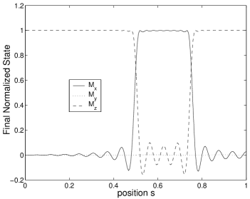
Figure 6: Results of pulse sequence designed to produce uniform $\frac{\pi}{2}$ rotation about $y$ axis over the range $0.5\leq s\leq 0.75$. The sequence was applied to the initial state $M(0)=[0\ 0\ 1]^{T}$, and the plot shows the final state as a function of $s$ after propagating the Bloch equations.

The ripples appearing in Figure 6 result from the ripples in the approximation of the sharp slice selective profile using a Fourier Series. One method used to overcome this in practice is to allow for a ramp between the $0$ and $\frac{\pi}{2}$ level on the slice.

IV Control Laws Involving Position and rf Inhomogeneity

We now come back to the problem of considering the full version of the Bloch equations (1) including the two dispersion parameters $s$ and $\epsilon$. Rewriting (1) in terms of the generators of rotation we have

$$\frac{d}{dt}\left[\begin{array}[]{c}M_{x}\\ M_{y}\\ M_{z}\end{array}\right]=(G(t)s\Omega_{z}+\epsilon u(t)\Omega_{y}+\epsilon v(t)\Omega_{x})\left[\begin{array}[]{c}M_{x}\\ M_{y}\\ M_{z}\end{array}\right]$$ (60)

where the state vector is now a function of both parameters $s$ and $\epsilon$. The control task is to choose $u(t)\in\Re$, $v(t)\in\Re$, and $G(t)\in\Re$ to effect a desired rotation $\phi(s,\epsilon)$. Proceeding along the lines of the previous two sections, consider generating the propagators

$$U_{1k} = \exp(\pi k_{1}s\Omega_{z})\exp(\frac{1}{4}\epsilon\beta_{k}\Omega_{y})\exp(-\pi k_{1}s\Omega_{z})$$ (61)

$$= \exp(\frac{1}{4}\epsilon\beta_{k}(\cos(\pi k_{1}s)\Omega_{y}-\sin(\pi k_{1}s)\Omega_{x}))$$

and

$$U_{2k} = \exp(-\pi k_{1}s\Omega_{z})\exp(\frac{1}{4}\epsilon\beta_{k}\Omega_{y})\exp(\pi k_{1}s\Omega_{z})$$ (62)

$$= \exp(\frac{1}{4}\epsilon\beta_{k}(\cos(\pi k_{1}s)\Omega_{y}+\sin(\pi k_{1}s)\Omega_{x}))$$

Within a first order approximation for the exponentials, we have the approximate total propagator

$$U_{1k}U_{2k}\approx\exp(\frac{1}{2}\epsilon\beta_{k}\cos(\pi k_{1}s)\Omega_{y})$$ (63)

Building on this, we can produce the propagator

$$U_{3k} = \exp(\pi k_{2}\epsilon\Omega_{x})U_{1k}U_{2k}\exp(-\pi k_{2}\epsilon\Omega_{x})$$

$$\approx \exp(\frac{1}{2}\epsilon\beta_{k}\cos(\pi k_{1}s)(\cos(\pi k_{2}\epsilon)\Omega_{y}-\sin(\pi k_{2}\epsilon)\Omega_{z}))$$

Similarly, we can produce

$$U_{4k} = \exp(-\pi k_{2}\epsilon\Omega_{x})U_{1k}U_{2k}\exp(\pi k_{2}\epsilon\Omega_{x})$$

$$\approx \exp(\frac{1}{2}\epsilon\beta_{k}\cos(\pi k_{1}s)(\cos(\pi k_{2}\epsilon)\Omega_{y}+\sin(\pi k_{2}\epsilon)\Omega_{z}))$$

so that we can approximately produce the total propagator

$$U_{k} = U_{3k}U_{4k}$$ (64)

$$\approx \exp(\epsilon\beta_{k}\cos(\pi k_{1}s)\cos(\pi k_{2}\epsilon)\Omega_{y})$$

within the approximation for the exponentials. We can use the method previously discussed in the case when $\beta_{k}$ is too large for the approximation to be valid. Producing the propagator $U_{k}$ for different values of $k_{1}$, $k_{2}$, and $\beta_{k}$ results in the net propagator

$$U=\prod_{\{k_{1},k_{2}\}}\exp(\epsilon\beta_{k}\cos(\pi k_{1}s)\cos(\pi k_{2}\epsilon)\Omega_{y})$$ (65)

A choice of $k_{1}$, $k_{2}$, and $\beta_{k}$ so that

$$\sum_{\{k_{1},k_{2}\}}\beta_{k}\cos(\pi k_{1}s)\cos(\pi k_{2}\epsilon)\approx\frac{\phi(s,\epsilon)}{\epsilon}$$ (66)

where $\phi(s,\epsilon)$ is the desired position $s$ and rf inhomogeneity parameter $\epsilon$ dependent rotation angle, results in an approximate desired evolution for the Bloch equations (60).

Analogous arguments show we may approximately produce a rotation around the $x$ axis of the Bloch sphere

$$U_{k}=\exp(\epsilon\beta_{k}\cos(\pi k_{1}s)\cos(\pi k_{2}\epsilon)\Omega_{x})$$ (67)

and may thus approximately generate a net propagator

$$U=\prod_{\{k_{1},k_{2}\}}\exp(\epsilon\beta_{k}\cos(\pi k_{1}s)\cos(\pi k_{2}\epsilon)\Omega_{x})$$ (68)

and thus approximately produce a desired position $s$ and rf inhomogeneity parameter $\epsilon$ rotation around the $x$ axis of the Bloch sphere. Since any rotation on the unit sphere can be decomposed in terms of Euler angles, an arbitrary $(s,\epsilon)$ dependent rotation can be approximately produced using these methods.

V Conclusions

In this paper we have provided new methods to design control laws for the Bloch equations when certain dispersion parameters are present in the system dynamics. These methods are of utmost practical importance in the fields of NMR spectroscopy and NMR imaging, and can be implemented in many well known experiments immediately. The methods presented in the paper allow the design of a compensating control law (pulse sequence) that will compensate for dispersions in the system dynamics while providing a clear tradeoff for the control law designer between total time required for the sequence and amplitude of the available controls.

References

• [1] J.S. Li and N. Khaneja, Noncommuting Vector Fields, Polynomial Approximations, and Control of Inhomogeneous Quantum Ensembles, Physical Review A, vol. 73, no. 030302 2006.
• [2] M. Bernstein, K. King, and X. Zhou, Handbook of MRI Pulse Sequences, Elsevier Academic Press, San Diego, USA, 2004.
• [3] J. Pauly, P. Le Roux, and D. Nishimura, Parameter Relations for the Shinnar-Le Roux Selective Excitation Pulse Design Algorithm, IEEE Transactions on Medical Imaging, vol. 10, no. 1 1991, pp 53-64.
• [4] J. Cavanagh, W. Fairbrother, A. Palmer, and N. Skelton, Protein NMR Spectroscopy, Academic Press, San Diego, USA, 1996.
• [5] M.H. Levitt, Composite pulses, Prog. NMR Spectroscopy vol. 18, 1986, pp 61-122.
• [6] R. Tycko, Broadband Population Inversion, Physical Review Letters, vol. 51, 1983, pp 775-777.
• [7] R. Tycko, N.M. Cho, E. Schneider, and A. Pines, Composite Pulses Without Phase Distortion, Journal of Magnetic Resonance, vol. 61, 1985, pp 90-101.
• [8] A.J. Shaka, and R. Freeman, Composite Pulses With Dual Compensation, Journal of Magnetic Resonance vol. 55, 1983, pp 487-493.
• [9] M. Levitt and R. Freeman, NMR Population Inversion Using a Composite Pulse, Journal of Magnetic Resonance vol. 33, 1979, pp 473.
• [10] M. Levitt and R.R. Ernst, Composite Pulses Constructed by a Recursive Expansion Procedure, Journal of Magnetic Resonance vol. 55, 1983, pp 247.
• [11] M. Garwood and Y. Ke, Symmetric Pulses to Induce Arbitrary Flip Angles with Compensation for rf Inhomogeneity and Resonance Offsets, Journal of Magnetic Resonance, vol. 94, 1991, pp 511-525.
• [12] T.E. Skinner, T. Reiss, B. Luy, N. Khaneja, and S.J. Glaser, Application of Optimal Control Theory to the Design of Broadband Excitation Pulses for High Resolution NMR, Journal of Magnetic Resonance vol. 163, 2003, pp 8-15.
• [13] K. Kobzer, T.E. Skinner, N. Khaneja, S.J. Glaser, and B. Luy, Exploring the Limits of Broadband Excitation and Inversion Pulses, Journal of Magnetic Resonance vol. 170, 2004, 236-243.
• [14] K. Kobzar, B. Luy, N. Khaneja, and S.J. Glaser, Pattern Pulses: Design of Arbitrary Excitation Profiles as a Function of Pulse Amplitude and Offset, Journal of Magnetic Resonance, vol. 173, 2005, pp 229-235.
• [15] M.S. Silver, R.I. Joseph, C.N. Chen, V.J. Sank, and D.I. Hoult, Selective Population Inversion in NMR, Nature vol. 310, 1984, pp 681-683.
• [16] M. Shinnar and J.S. Leigh, The Application of Spinors to Pulse Synthesis and Analysis, Magnetic Resonance Med. vol. 12, 1989, pp 93-98.
• [17] P. Le Roux, Exact Synthesis of Radio Frequency Waveforms, Proc. 7th SMRM 1988, pp 1049.
• [18] S. Conolly, D. Nishimura, and A. Macovski, Optimal Control to the Magnetic Resonance Selective Excitation Problem IEEE Trans. Med. Imag. MI-5 1986, pp 106-115.
• [19] M. Nielsen and I. Chuang, Quantum Computation and Quantum Information, Quantum Computation and Qunatum Information, Cambridge University Press, Cambridge, England, 2000.