Boosted Black Holes on Kaluza-Klein Bubbles

Abstract

We construct an exact stationary solution of black hole – bubble sequence in the five dimensional Kaluza-Klein theory by using solitonic solution generating techniques. The solution describes two boosted black holes with topology $S^{3}$ on a Kaluza-Klein bubble and has a linear momentum component in the compactified direction. The ADM mass and the linear momentum depend on the two boosted velocity parameters of black holes. In the effective four dimensional theory, the solution has an electric charge which is proportional to the linear momentum. The solution includes the static solution found by Elvang and Horowitz and a limit of single boosted black string.

I Introduction

Kaluza-Klein (KK) theory is the five dimensional theory of gravity which unifies Einstein’s four-dimensional theory of gravity and Maxwell’s electromagnetic theory KK ; Overduin:1998pn . The spacetime is asymptotically the product of the four-dimensional Minkowski spacetime ${\cal M}^{3,1}$ and a circle $S^{1}$. The extra dimension with $S^{1}$ is compactified too small for us to observe it. This type of compactification of the extra dimensions are also extended to the supergravity theories and the superstrings.

The studies on black holes in the KK theory have attracted much attention since they admit much richer structures than asymptotically flat higher dimensional black holes. For example, such black holes can have the horizons with the topologies of the squashed $S^{3}$ and the lens space $L(2;1)=S^{3}/{\mathbb{Z}}_{2}$ IM ; Ishihara . Another exciting aspects of the KK theory are the existence of KK bubbles. In Ref. Elvang:2004iz , a large class of five- and six-dimensional static solutions which describe the sequences of the black holes and KK bubbles were constructed and analyzed. The KK bubble was first found by Witten as the end state of the KK vacuum decay Witten . The first solution of the sequence of black holes and bubbles is the combination of the static black hole and KK bubble weyl . Elvang and Horowitz found and analyzed the two black holes sitting on the KK bubble EH . The static equilibrium of the spacetime is maintained by the existence of the KK bubbles which balance the attractive force of black holes.

In the previous article, we obtained the new five-dimensional vacuum solution of rotating black holes on the KK bubble Tomizawa:2007mz . This solution is the extension of the static solution found by Elvang and Horowitz to a stationary solution, which has an ADM mass and an ADM angular momentum. We used two different types of solution generating methods to obtain the solution. One is called Bäcklund transformation Harrison ; Neugebauer , which is basically the technique to generate a new solution of the Ernst equation. The other is the inverse scattering technique, which Belinski and Zakharov Belinskii developed as an another type of solution-generating technique. In this several years, these techniques have been applied to generate and to reproduce five-dimensional black hole solutions with asymptotically flatness Mishima ; MI2 ; MI3 ; Koikawa ; Tomizawa ; Azuma ; Pomeransky:2005sj ; Tomizawa2 ; Pomeransky2 ; EF . The relation between these two methods was examined in the context of the five-dimensional spacetime Tomizawa3 . It was shown that the two-solitonic solutions generated from an arbitrary diagonal seed by the Bäcklund transformation coincide with those with a single angular momentum generated from the same seed by the inverse scattering method.

In this article we generate another type of stationary solution which describes boosted black holes on the KK-bubble as a vacuum solution in the five-dimensional Einstein equations by using both solitonic methods. It should be noted that this solution cannot be generated by the simple boost transformation of the static solution because the boosted solution always has closed timelike curves around the bubble. The solution has a linear momentum in the compact direction and does not have an ADM angular momentum. This is the reason why we call the solution boosted black holes on KK bubble. In the four dimensional effective theory, this solution has an electric charge which is proportional to the linear momentum. There is a limit of single black hole without KK bubble in this solution. This limiting solution exactly corresponds to the simply boosted black string Dobiasch:1981vh ; Gibbons:1985ac ; Cvetic:1995sz ; Chamblin:1996kw whose thermodynamical properties are studied recently Kastor:2007wr . The solution with two momentum components will be generated by the inverse scattering method

This article is organized as follows: In Sec.II, we give a new solution generated by the solitonic methods. We introduce only the construction by the Bäclund transformation in this section, while the other construction is briefly mentioned in Appendix A. In Sec.III, we investigate the properties of the solution. In Sec.IV, we give the summary and discussion of this article. In Appendix, we give the solution generated by the inverse scattering method and the relation between these solutions.

II Solutions

At first we briefly present the solution obtained by the Bäcklund transformation which was applied the five dimensional case Mishima . Using this method, we can generate axially symmetric solutions of five-dimensional vacuum Einstein equations. See Mishima for the detail of the solution generating method.

We start from the following form of a seed static metric

$$ds^{2}=e^{-T^{(0)}}\left[-e^{S^{(0)}}(dt)^{2}+e^{-S^{(0)}}\rho^{2}(d\phi)^{2}+e^{2\gamma^{(0)}-S^{(0)}}\left(d\rho^{2}+dz^{2}\right)\right]+e^{2T^{(0)}}(d\psi)^{2},$$ (1)

with seed functions

$$S^{(0)} = {U}_{\lambda\sigma}-\tilde{U}_{\eta_{1}\sigma}+2\tilde{U}_{\eta_{2}\sigma}$$ (2)

$$= -\tilde{U}_{\lambda\sigma}-\tilde{U}_{\eta_{1}\sigma}+2\tilde{U}_{\eta_{2}\sigma}+\ln\rho$$

$$T^{(0)} = {U}_{\lambda\sigma}+\tilde{U}_{\eta_{1}\sigma}$$ (3)

$$= -\tilde{U}_{\lambda\sigma}+\tilde{U}_{\eta_{1}\sigma}+\ln\rho,$$

where we assume $\eta_{1}<\eta_{2}<\lambda<1$. The function $U_{d}$ is defined as $U_{d}:=\frac{1}{2}\ln\left[\,R_{d}-(z-d)\,\right]$ and the function ${\tilde{U}}_{d}$ is defined as ${\tilde{U}}_{d}:=\frac{1}{2}\ln\left[\,R_{d}+(z-d)\,\right]$ where $R_{d}:=\sqrt{\rho^{2}+(z-d)^{2}}$. Here we take the coordinate $\phi$ as a Kaluza-Klein compactified direction. As explained later, the solitonic solution has two event horizons at $\eta_{1}\sigma\leq z\leq\eta_{2}\sigma$ and $-\sigma\leq z\leq\lambda\sigma$ and a Kaluza-Klein bubble at $\eta_{2}\sigma\leq z\leq-\sigma$, where the Kaluza-Klein circles shrink to zero. The metric of the solitonic solution can be written in the following form

$$ds^{2} = e^{-T}\left[-e^{S}(dt-\omega d\phi)^{2}+e^{-S}\rho^{2}(d\phi)^{2}+e^{2\gamma-S}\left(d\rho^{2}+dz^{2}\right)\right]+e^{2T}(d\psi)^{2}.$$ (4)

The function $T$ is derived from the seed functions

$$T=-\tilde{U}_{\lambda\sigma}+\tilde{U}_{\eta_{1}\sigma}+\ln\rho.$$ (5)

The other metric functions for the five-dimensional metric (4) are obtained by using the formulas shown by Castejon-Amenedo:1990b ,

$$e^{S} = e^{S^{(0)}}\frac{A}{B},$$ (6)

$$\omega = 2\sigma e^{-S^{(0)}}\frac{C}{A}-C_{1},$$ (7)

$$e^{2\gamma} = C_{2}(x^{2}-1)^{-1}Ae^{2\gamma^{\prime}},$$ (8)

where $C_{1}$ and $C_{2}$ are constants and $A$, $B$ and $C$ are given by

$$A = \frac{1}{(2\sigma)^{2}}\left\{\left(e^{2{\tilde{U}}_{-\sigma}}+e^{2U_{\sigma}}\right)\left(e^{2{\tilde{U}}_{\sigma}}+e^{2U_{-\sigma}}\right)(1+ab)^{2}-\left(e^{2{\tilde{U}}_{-\sigma}}-e^{2{\tilde{U}}_{\sigma}}\right)\left(e^{2U_{\sigma}}-e^{2U_{-\sigma}}\right)(b-a)^{2}\right\},$$

$$B = \frac{1}{(2\sigma)^{2}}\left\{\left[\left(e^{2{\tilde{U}}_{-\sigma}}+e^{2U_{\sigma}}\right)+\left(e^{2{\tilde{U}}_{\sigma}}+e^{2U_{-\sigma}}\right)ab\right]^{2}+\left[\left(e^{2{\tilde{U}}_{-\sigma}}-e^{2{\tilde{U}}_{\sigma}}\right)a-\left(e^{2U_{\sigma}}-e^{2U_{-\sigma}}\right)b\right]^{2}\right\},$$

$$C = \frac{1}{(2\sigma)^{3}}\left\{\left(e^{2{\tilde{U}}_{-\sigma}}+e^{2U_{\sigma}}\right)\left(e^{2{\tilde{U}}_{\sigma}}+e^{2U_{-\sigma}}\right)(1+ab)\left(\left(e^{2U_{\sigma}}-e^{2U_{-\sigma}}\right)b-\left(e^{2{\tilde{U}}_{-\sigma}}-e^{2{\tilde{U}}_{\sigma}}\right)a\right)\right.$$

$$\left.+\left(e^{2{\tilde{U}}_{-\sigma}}-e^{2{\tilde{U}}_{\sigma}}\right)\left(e^{2U_{\sigma}}-e^{2U_{-\sigma}}\right)(b-a)\left(\left(e^{2{\tilde{U}}_{-\sigma}}+e^{2U_{\sigma}}\right)-\left(e^{2{\tilde{U}}_{\sigma}}+e^{2U_{-\sigma}}\right)ab\right)\right\}.$$

The functions $a$ and $b$, which are auxiliary potential to obtain the new Ernst potential by the transformation, are given by

$$a = \alpha\sqrt{\frac{(e^{2{\tilde{U}}_{-\sigma}}+e^{2U_{\sigma}})(e^{2U_{\sigma}}-e^{2U_{-\sigma}})}{(e^{2{\tilde{U}}_{\sigma}}+e^{2U_{-\sigma}})(e^{2{\tilde{U}}_{-\sigma}}-e^{2{\tilde{U}}_{\sigma}})}}\frac{e^{{\tilde{U}}_{{\lambda}\sigma}}}{e^{2U_{\sigma}}+e^{2{\tilde{U}}_{{\lambda}\sigma}}}\frac{e^{{\tilde{U}}_{\eta_{1}\sigma}}}{e^{2U_{\sigma}}+e^{2{\tilde{U}}_{\eta_{1}\sigma}}}\left(\frac{e^{2U_{\sigma}}+e^{2{\tilde{U}}_{\eta_{2}\sigma}}}{e^{{\tilde{U}}_{\eta_{2}\sigma}}}\right)^{2},$$ (9)

$$b = \beta\sqrt{\frac{(e^{2{\tilde{U}}_{-\sigma}}+e^{2U_{\sigma}})(e^{2{\tilde{U}}_{-\sigma}}-e^{2{\tilde{U}}_{\sigma}})}{(e^{2{\tilde{U}}_{\sigma}}+e^{2U_{-\sigma}})(e^{2U_{\sigma}}-e^{2U_{-\sigma}})}}\frac{e^{2U_{-\sigma}}+e^{2{\tilde{U}}_{{\lambda}\sigma}}}{e^{{\tilde{U}}_{{\lambda}\sigma}}}\frac{e^{2U_{-\sigma}}+e^{2{\tilde{U}}_{\eta_{1}\sigma}}}{e^{{\tilde{U}}_{\eta_{1}\sigma}}}\left(\frac{e^{{\tilde{U}}_{\eta_{2}\sigma}}}{e^{2U_{-\sigma}}+e^{2{\tilde{U}}_{\eta_{2}\sigma}}}\right)^{2}.$$ (10)

In addition the function $\gamma^{\prime}$ is obtained as

$${\gamma}^{\prime} = {\gamma}^{\prime}_{\sigma,\sigma}+{\gamma}^{\prime}_{-\sigma,-\sigma}+{\gamma}^{\prime}_{\lambda\sigma,\lambda\sigma}+{\gamma}^{\prime}_{\eta_{1}\sigma,\eta_{1}\sigma}+{\gamma}^{\prime}_{\eta_{2}\sigma,\eta_{2}\sigma}$$ (11)

$$-2{\gamma}^{\prime}_{\sigma,-\sigma}-{\gamma}^{\prime}_{\sigma,\lambda\sigma}-{\gamma}^{\prime}_{\sigma,\eta_{1}\sigma}+2{\gamma}^{\prime}_{\sigma,\eta_{2}\sigma}+{\gamma}^{\prime}_{-\sigma,\lambda\sigma}+{\gamma}^{\prime}_{-\sigma,\eta_{1}\sigma}-2{\gamma}^{\prime}_{-\sigma,\eta_{2}\sigma}$$

$$-{\gamma}^{\prime}_{\lambda\sigma,\eta_{1}\sigma}-{\gamma}^{\prime}_{\lambda\sigma,\eta_{2}\sigma}-{\gamma}^{\prime}_{\eta_{1}\sigma,\eta_{2}\sigma}$$

$$+\tilde{U}_{\sigma}-\tilde{U}_{-\sigma}-2\tilde{U}_{\lambda\sigma}+\tilde{U}_{\eta_{1}\sigma}+\tilde{U}_{\eta_{2}\sigma}+\ln\rho,$$

where

$${\gamma}^{\prime}_{cd}=\frac{1}{2}{\tilde{U}}_{c}+\frac{1}{2}{\tilde{U}}_{d}-\frac{1}{4}\ln[R_{c}R_{d}+(z-c)(z-d)+\rho^{2}].$$ (12)

The constants $C_{1}$ and $C_{2}$ are chosen as follows

$$C_{1}=0,\quad C_{2}=\frac{1}{(1+\alpha\beta)^{2}},$$ (13)

to avoid the global boost of the spacetime and to set the period of $\psi$ to $2\pi$, respectively. Also the integration constants $\alpha$ and $\beta$ should be decided as

$$\alpha^{2}=\frac{(1-\lambda)(1-\eta_{1})}{(1-\eta_{2})^{2}},\quad\beta=0,$$ (14)

to remove the singularity at $z=\sigma$ on $z$-axis and closed timelike curves around the bubble, respectively.

III Properties

Next, we investigate the properties of the solution satisfying the conditions (13) and (14). In particular, we study the asymptotic structure, the geometry of two black hole horizons and a bubble and the limits of the static case and the single boosted black hole.

III.1 Asymptotic structure

In order to investigate the asymptotic structure of the solution, let us introduce the coordinate $(r,\theta)$ defined as

$$\rho=r\sin\theta,\quad z=r\cos\theta,$$ (15)

where $0\leq\theta<2\pi$ and $r$ is a four-dimensional radial coordinate in the neighborhood of the spatial infinity. For the large $r\to\infty$, each component behaves as

$$g_{tt}\simeq-1+\frac{(2-\eta_{1}+\eta_{2})\sigma}{r},$$ (16)

$$g_{\rho\rho}=g_{zz}\simeq 1+\frac{(\lambda-\eta_{1})\sigma}{r},$$ (17)

$$g_{t\phi}\simeq-\frac{2\alpha\sigma}{r},$$ (18)

$$g_{\phi\phi}\simeq 1+\frac{(2+\eta_{2}-\lambda)\sigma}{r},$$ (19)

$$g_{\psi\psi}\simeq r^{2}\sin^{2}\theta\left(1-\frac{(\eta_{1}-\lambda)\sigma}{r}\right).$$ (20)

Hence, the leading order of the metric takes the form

$$ds^{2}\simeq-dt^{2}+dr^{2}+r^{2}(d\theta^{2}+\sin^{2}\theta d\psi^{2})+d\phi^{2}.$$ (21)

Therefore, the spacetime has the asymptotic structure of the direct product of the four-dimensional Minkowski spacetime and $S^{1}$. The $S^{1}$ at infinity is parameterized by $\phi$ and the size $\Delta\phi$ is given in III.3.

III.2 Mass and momentum

Next, we compute the total mass and the linear momentum of the spacetime. It should be noted that since the asymptotic structure is ${\cal M}^{3,1}\times S^{1}$, the ADM mass and momentum are given by the surface integral over the spatial infinity with the topology of $S^{2}\times S^{1}$. In order to compute these quantities, we introduce asymptotic Cartesian coordinates $(x,y,z,\phi)$, where $x=\rho\cos\psi$ and $y=\rho\sin\psi$. Then, the ADM mass and momentum in the $\phi$ direction are given by

$${\cal M}_{\rm ADM}=\frac{1}{16\pi}\int_{S^{2}\times S^{1}}(\partial_{j}h_{ij}-\partial_{i}h_{jj})dS_{i},$$ (22)

$${\cal P}=\frac{1}{16\pi}\int_{S^{2}\times S^{1}}\partial_{i}h_{0\phi}dS_{i}$$ (23)

respectively. Here $h_{\mu\nu}$ is deviation from the five-dimensional flat metric $\eta_{\mu\nu}$ near infinity,

$$g_{\mu\nu}=\eta_{\mu\nu}+h_{\mu\nu}.$$ (24)

The Latin index $i,j$ runs $x,y,z$ and $\phi$ and the Greek indeces $\mu,\nu,\alpha$ and $\beta$ label $t,x,y,z$ and $\phi$. Then, the ADM mass of the solution is computed as

$${\cal M}_{ADM}=\frac{(\lambda-2\eta_{1}+\eta_{2}+2)\sigma}{4}\Delta\phi.$$ (25)

It should be noted that the ADM mass is non-negative. The linear momentum becomes

$${\cal P}=-\frac{\alpha\sigma}{2}\Delta\phi.$$ (26)

The electric charge of four dimensional effective theory is proportional to the linear momentum per unit $\phi$ length. We define it as

$$Q_{4}=\alpha\sigma.$$ (27)

III.3 Black holes and bubble

Here, for the solution, we consider the rod structure developed by Harmark Harmark and Emparan and Reall weyl . The rod structure at $\rho=0$ is illustrated in FIG.1. (i) The finite timelike rod $[\eta_{1}\sigma,\eta_{2}\sigma]$ and $[-\sigma,\lambda\sigma]$ denote the locations of black hole horizons. These timelike rods have directions $v_{1}=(1,\Omega_{1},0)$ and $v_{2}=(1,\Omega_{2},0)$. We call $\Omega_{1}$ and $\Omega_{2}$ boost velocity parameters. These are given by

$$\Omega_{1}=\frac{2\alpha}{1-\eta_{1}},$$ (28)

for $\eta_{1}\sigma<z<\eta_{2}\sigma$ and

$$\Omega_{2}=\frac{\alpha(1-\eta_{2})^{2}}{2(1-\eta_{1})},$$ (29)

for $-\sigma<z<\lambda\sigma.$ Here, it should be noted that $\Omega_{1}$ and $\Omega_{2}$ have the same signature. Therefore, two black holes are boosted along the same direction. (ii) The finite spacelike rod $[\eta_{2}\sigma,-\sigma]$ which corresponds to a Kaluza-Klein bubble has the direction $v=(0,1,0)$. In order to avoid conical singularity for $z\in[\eta_{2}\sigma,-\sigma]$ and $\rho=0$, $\phi$ has the periodicity of

$$\frac{\Delta\phi}{2\pi} = \lim_{\rho\rightarrow\infty}\sqrt{\frac{\rho^{2}g_{\rho\rho}}{g_{\phi\phi}}}$$ (30)

$$= 2\sigma\frac{\eta_{2}+1}{\eta_{2}-1}\sqrt{\frac{(\lambda-\eta_{1})(\lambda-\eta_{2})(\eta_{1}-1)}{\eta_{1}+1}}.$$

(iii) The semi-infinite spacelike rods $[-\infty,\eta_{1}\sigma]$ and $[\lambda\sigma,\infty]$ have the direction $v=(0,0,1)$. In order to avoid conical singularity, $\psi$ has the periodicity of

$$\Delta\psi=2\pi.$$ (31)

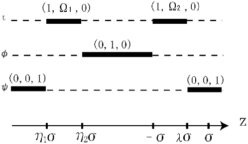
Figure 1: Rod structure of boosted black holes on a Kaluza-Klein bubble. The finite timelike rods $[\eta_{1}\sigma,\eta_{2}\sigma]$ and $[-\sigma,\lambda\sigma]$ correspond to black holes with boost velocities $\Omega_{1}$ and $\Omega_{2}$, respectively. The finite spacelike rod $[\eta_{2}\sigma,-\sigma]$ denotes a Kaluza-Klein bubble, where Kaluza-Klein circles shrink to zero.

Here, we write the induced metrics of the event horizons and the bubble. For $\eta_{1}\sigma<z<\eta_{2}\sigma$, the induced metric becomes

$$g_{tt} = \frac{\Omega_{1}^{2}(z-\sigma)(z+\sigma)(z-\eta_{2}\sigma)}{(z-\lambda\sigma)(z+\sigma)^{2}-\Omega_{1}^{2}(z-\eta_{1}\sigma)(z-\eta_{2}\sigma)^{2}},$$ (32)

$$g_{t\phi} = -\frac{\Omega_{1}(z-\sigma)(z+\sigma)(z-\eta_{2}\sigma)}{(z-\lambda\sigma)(z+\sigma)^{2}-\Omega_{1}^{2}(z-\eta_{1}\sigma)(z-\eta_{2}\sigma)^{2}},$$ (33)

$$g_{zz} = \frac{\sigma^{2}(1-\eta_{1})(\eta_{2}-\eta_{1})(\lambda-\eta_{1})((z-\lambda\sigma)(z+\sigma)^{2}-\Omega_{1}^{2}(z-\eta_{1}\sigma)(z-\eta_{2}\sigma)^{2})}{(1+\eta_{1})(z-\sigma)(z+\sigma)(z-\eta_{1}\sigma)(z-\eta_{2}\sigma)(z-\lambda\sigma)},$$ (34)

$$g_{\phi\phi} = \frac{(z-\sigma)(z+\sigma)(z-\eta_{2}\sigma)}{(z-\lambda\sigma)(z+\sigma)^{2}-\Omega_{1}^{2}(z-\eta_{1}\sigma)(z-\eta_{2}\sigma)^{2}},$$ (35)

$$g_{\psi\psi}=-4(z-\eta_{1}\sigma)(z-\lambda\sigma),$$ (36)

Since the $\phi$ circles shrink to zero at $z=\eta_{2}\sigma$ and $\psi$ circles shrink to zero at $z=\eta_{1}\sigma$, the spatial cross section of this black hole horizon is topologically $S^{3}$. The area of the event horizon is

$$A_{1} = 8\pi^{2}\sigma^{2}\sqrt{\frac{(1-\eta_{1})(\lambda-\eta_{1})(\eta_{2}-\eta_{1})^{3}}{-1-\eta_{1}}}\Delta\phi$$ (37)

$$= 16\pi^{2}\sigma^{3}\frac{(1-\eta_{1})(-1-\eta_{2})(\eta_{2}-\eta_{1})^{\frac{3}{2}}(\lambda-\eta_{1})(\lambda-\eta_{2})^{\frac{1}{2}}}{(-1-\eta_{1})(1-\eta_{2})}.$$

For $-\sigma<z<\lambda\sigma$, the induced metric takes the following form

$$g_{tt} = \frac{\Omega_{2}^{2}(z-\sigma)(z+\sigma)(z-\eta_{2}\sigma)}{(z-\lambda\sigma)(z-\eta_{2}\sigma)^{2}-\Omega_{2}^{2}(z+\sigma)^{2}(z-\eta_{1}\sigma)},$$ (38)

$$g_{t\phi} = -\frac{\Omega_{2}(z-\sigma)(z+\sigma)(z-\eta_{2}\sigma)}{(z-\lambda\sigma)(z-\eta_{2}\sigma)^{2}-\Omega_{2}^{2}(z+\sigma)^{2}(z-\eta_{1}\sigma)},$$ (39)

$$g_{zz} = -\frac{4\sigma^{2}(1-\eta_{1})(\eta_{1}-\lambda)(\eta_{2}-\lambda)((z-\lambda\sigma)(z-\eta_{2}\sigma)^{2}-\Omega_{2}^{2}(z+\sigma)^{2}(z-\eta_{1}\sigma))}{(1-\eta_{2})^{2}(1+\lambda)(z-\sigma)(z+\sigma)(z-\eta_{1}\sigma)(z-\eta_{2}\sigma)(z-\lambda\sigma)},$$ (40)

$$g_{\phi\phi} = \frac{(z-\sigma)(z+\sigma)(z-\eta_{2}\sigma)}{(z-\lambda\sigma)(z-\eta_{2}\sigma)^{2}-\Omega_{2}^{2}(z+\sigma)^{2}(z-\eta_{1}\sigma)},$$ (41)

$$g_{\psi\psi}=-4(z-\eta_{1}\sigma)(z-\lambda\sigma),$$ (42)

Since the $\phi$ circles shrink to zero at $z=-\sigma$ and $\psi$ circles shrink to zero at $z=\lambda\sigma$, the spatial cross section of this black hole horizon is also topologically $S^{3}$. The area of this event horizon is

$$A_{2} = 16\pi^{2}\sigma^{2}\sqrt{(1-\eta_{1})(\lambda-\eta_{1})(\lambda-\eta_{2})(\lambda+1)}\Delta\phi$$ (43)

$$= 32\pi^{2}\sigma^{3}\frac{(1-\eta_{1})(-1-\eta_{2})(\lambda-\eta_{1})(\lambda-\eta_{2})(\lambda+1)^{\frac{1}{2}}}{(1-\eta_{2})(-1-\eta_{1})^{\frac{1}{2}}}.$$

For $\eta_{2}\sigma<z<-\sigma$, the induced metric on the bubble can be written in the form

$$g_{tt}=-\frac{(z+\sigma)(z-\eta_{2}\sigma)}{(z-\sigma)(z-\eta_{1}\sigma)},$$ (44)

$$g_{t\phi}=-\frac{\sigma^{2}\Omega_{2}\rho^{2}}{(z+\sigma)(z-\eta_{2}\sigma)(z-\lambda\sigma)},$$ (45)

$$g_{zz}=\sigma^{2}\frac{(1-\eta_{1})(1+\eta_{2})^{2}(\lambda-\eta_{1})(\lambda-\eta_{2})(z-\sigma)}{(1+\eta_{1})(1-\eta_{2})^{2}(z+\sigma)(z-\eta_{2}\sigma)(z-\lambda\sigma)},$$ (46)

$$g_{\phi\phi}=-\frac{(z-\sigma)\rho^{2}}{4(z-\eta_{2}\sigma)(z-\lambda\sigma)(z+\sigma)},$$ (47)

$$g_{\psi\psi}=-4(z-\eta_{1}\sigma)(z-\lambda\sigma),$$ (48)

The $\phi$ circle vanishes for $z\in[\eta_{2}\sigma,-\sigma]$ and $\rho=0$, which means that there exists a Kaluza-Klein bubble in this region. Since the $\psi$ circle does not vanish at $z=\eta_{2}\sigma$ and $z=\lambda\sigma$, this bubble on the time slice is topologically a cylinder $S^{1}\times R$. Therefore, there exist a Kaluza-Klein bubble between two boosted black holes with topology of $S^{3}$. The proper distance between the two black hols is

$$s=\sigma\frac{(\eta_{2}+1)}{(\eta_{2}-1)}\sqrt{\frac{(\eta_{1}-1)(\lambda-\eta_{1})(\lambda-\eta_{2})}{(\eta_{1}+1)}}\int^{-\sigma}_{\eta_{2}\sigma}dz\sqrt{-\frac{z-\sigma}{(z+\sigma)(z-\eta_{2}\sigma)(z-\lambda\sigma)}}.$$ (49)

The Kaluza-Klein bubble is significant to keep the balance of two black holes and achieve the solution without any strut structures and singularities. This property resembles that of the solution given by Elvang and Horowitz EH and the extension of it with rotation Tomizawa:2007mz . In the next subsection, we will show that the static limit of the solution coincides with the solution given by Elvang and Horowitz.

At the end of this subsection we rewrite the ADM mass (25) and the electric charge (27) by using boost velocities $\Omega_{1}$ and $\Omega_{2}$. The ADM mass is

$$\frac{M_{ADM}}{\Delta\phi} = \frac{(\lambda-\eta_{1})\sigma}{2}\left(1+\frac{1-\lambda}{2(\lambda-\eta_{1})}\right)+\frac{(1+\eta_{2})\sigma}{4}$$ (50)

$$= m\left(1+\frac{\Omega_{1}\Omega_{2}}{2(1-\Omega_{1}\Omega_{2})}\right)+m_{0}\left(1-\sqrt{\frac{\Omega_{1}}{\Omega_{2}}}\right),$$

where $m=\frac{(\lambda-\eta_{1})\sigma}{2}$ and $m_{0}=\frac{\sigma}{2}$. The eclectic charge is

$$Q_{4}=\alpha\sigma=m\frac{\Omega_{1}}{1-\Omega_{1}\Omega_{2}}.$$ (51)

III.4 Static case

In this subsection, we consider the static case, which can be obtained by the choice of the parameter $\lambda=1$. Then, from Eq. (14) we see that $\alpha$ vanishes. Let us define the parameters $\tilde{a},\tilde{b}$ and $\tilde{c}$ as

$$\tilde{a}=\frac{2\lambda+1-\eta_{2}}{2}\sigma,\quad\tilde{b}=\frac{-1-\eta_{2}}{2}\sigma,\quad\tilde{c}=\frac{-1+\eta_{2}-2\eta_{1}}{2}\sigma.$$ (52)

It should be noted that $\lambda=1$ is equal to the condition $\sigma=(\tilde{a}-\tilde{b})/2$. Furthermore, let us shift an origin of the $z$-coordinate such that $z\to\tilde{z}:=z-(\eta_{2}-\lambda)\sigma/2$. Then, we obtain the metric

$$ds^{2} = -\frac{(R_{\tilde{b}}-(\tilde{z}-\tilde{b}))(R_{-\tilde{c}}-(\tilde{z}+\tilde{c}))}{(R_{\tilde{a}}-(\tilde{z}-\tilde{a}))(R_{-\tilde{b}}-(\tilde{z}+\tilde{b}))}dt^{2}+(R_{\tilde{a}}-(\tilde{z}-\tilde{a}))(R_{-\tilde{c}}-(\tilde{z}+\tilde{c}))d\psi^{2}$$ (53)

$$+\frac{R_{-\tilde{b}}-(\tilde{z}+\tilde{b})}{R_{\tilde{b}}-(\tilde{z}-\tilde{b})}d\phi^{2}+\frac{Y_{\tilde{a},-\tilde{c}}Y_{\tilde{b},-\tilde{b}}}{4R_{\tilde{a}}R_{\tilde{b}}R_{-\tilde{b}}R_{-\tilde{c}}}\sqrt{\frac{Y_{\tilde{a},\tilde{b}}Y_{-\tilde{b},-\tilde{c}}}{Y_{\tilde{a},-\tilde{b}}Y_{\tilde{b},-\tilde{c}}}}\frac{R_{\tilde{a}}-({\tilde{z}}-\tilde{a})}{R_{-\tilde{c}}-({\tilde{z}}+\tilde{c})}(d\rho^{2}+d\tilde{z}^{2}),$$

where the coordinate $z$ in the definition of $R_{d}$ is replaced with $\tilde{z}$. This coincides with the solution obtained by Elvang and Horowitz EH , which describes static black holes on the Kaluza-Klein bubble.

III.5 Boosted black string

The single boosted black string is achieved by taking the limit $\eta_{2}\rightarrow-1$. This solution corresponds to the electric charged black hole in the effective four dimensional theory Gibbons:1985ac ; Cvetic:1995sz ; Chamblin:1996kw . It can be easily confirmed that the ADM mass (50) and the electric charge (51) become well-known forms because $\Omega_{1}=\Omega_{2}$ when $\eta_{2}=-1$. The $3\times 3$ metric functions become the following form

$$g_{tt} = -\frac{R_{\lambda\sigma}+R_{\eta_{1}\sigma}-(2-\lambda-\eta_{1})\sigma}{R_{\lambda\sigma}+R_{\eta_{1}\sigma}+(\lambda-\eta_{1})\sigma},$$ (54)

$$g_{t\phi} = -\frac{2\sqrt{(1-\lambda)(1-\eta_{1})}\sigma}{R_{\lambda\sigma}+R_{\eta_{1}\sigma}+(\lambda-\eta_{1})\sigma},$$ (55)

$$g_{\phi\phi} = \frac{R_{\lambda\sigma}+R_{\eta_{1}\sigma}+(2-\lambda-\eta_{1})\sigma}{R_{\lambda\sigma}+R_{\eta_{1}\sigma}+(\lambda-\eta_{1})\sigma},$$ (56)

$$g_{\psi\psi} = \rho^{2}\frac{R_{\lambda\sigma}+R_{\eta_{1}\sigma}+(\lambda-\eta_{1})\sigma}{R_{\lambda\sigma}+R_{\eta_{1}\sigma}-(\lambda-\eta_{1})\sigma}.$$ (57)

Introducing the Schwarzschild radial coordinate as

$$r_{s}=\frac{R_{\lambda\sigma}+R_{\eta_{1}\sigma}}{2}+m,$$ (58)

we can derive a familiar expression of the boosted black string from the solitonic solution.

IV Summary and Discussion

Using the solitonic solution generating methods, we generated a new exact solution which describes a pair of boosted black holes in the compact direction on a Kaluza-Klein bubble as a vacuum solution in the five-dimensional Kaluza-Klein theory. This solution cannot be obtained by the simple boost transformation of the static black holes on Kaluza-Klein bubble. We also investigated the properties of this solution, particularly, its asymptotic structure, the geometry of the black hole horizons and the Kaluza-Klein bubble and the limits of single black string and static case. The asymptotic structure is the $S^{1}$ bundle over the four-dimensional Minkowski spacetime. Two black holes have the topological structure of $S^{3}$ and the bubble is topologically $S^{1}\times R$. The solution describes the physical situation such that two black holes have the boost velocity of the same direction and the bubble plays a role in holding two black holes. The ADM mass and the linear momentum of the solution can be written by the two boosted velocity parameters. In the static case, it coincides with the solution found by Elvang and Horowitz. The solution has a limit of single boosted black string.

In this article, we concentrated on the black hole solution with a linear momentum component. The solution with an angular momentum component has been derived in the previous paper Tomizawa:2007mz . The investigation on the solution with these two components is enormously challenging. In general, the inverse scattering method can generate a solution with two momentum components. We will give such a solution in our future article.

Appendix A Solutions generated by ISM

Following the techniques in the Ref Tomizawa ; Tomizawa2 ; Tomizawa3 , we construct a new Kaluza-Klein black hole solution. We consider the five-dimensional stationary and axisymmetric vacuum spacetimes which admit three commuting Killing vectors $\partial/\partial t$, $\partial/\partial\phi$ and $\partial/\partial\psi$, where $\partial/\partial t$ is a Killing vector field associated with time translation, $\partial/\partial\phi$ and $\partial/\partial\psi$ denote spacelike Killing vector fields with closed orbits. In such a spacetime, the metric can be written in the canonical form as

$$ds^{2}=g_{ij}dx^{i}dx^{j}+f(d\rho^{2}+dz^{2}),$$ (59)

where the metric components $g_{ij}$ and the metric coefficient $f$ are functions which depend on $\rho$ and $z$ only. The metric $g_{ij}$ satisfies the supplementary condition ${\rm det}\ g_{ij}=-\rho^{2}$. We begin with the following seed

$$ds^{2}=-\frac{R_{\eta_{2}\sigma}+z-\eta_{2}\sigma}{R_{\eta_{1}\sigma}+z-\eta_{1}\sigma}dt^{2}+\frac{R_{\lambda\sigma}+z-\lambda\sigma}{R_{\eta_{2}\sigma}+z-\eta_{2}\sigma}d\phi^{2}+\frac{R_{\eta_{1}\sigma}+z-\eta_{1}\sigma}{R_{\lambda\sigma}+z-\lambda\sigma}\rho^{2}d\psi^{2}+f(d\rho^{2}+dz^{2}),$$

(60)

where $R_{d}$ is defined as $R_{d}:=\sqrt{\rho^{2}+(z-d)^{2}}$. The parameters $\eta_{1},\eta_{2}$ and $\lambda$ satisfy the inequality $\eta_{1}<\eta_{2}<\lambda<1$ and $\sigma>0$. Instead of solving the L-A pair for the seed metric (60), it is sufficient to consider the following metric form

$$ds^{2}=-dt^{2}+g_{2}d\phi^{2}+g_{3}d\psi^{2}+f(d\rho^{2}+dz^{2}),$$ (61)

where $g_{2}$ and $g_{3}$ are given by

$$g_{2}=\frac{(R_{\eta_{1}\sigma}+z-\eta_{1}\sigma)(R_{\lambda\sigma}+z-\lambda\sigma)}{(R_{\eta_{2}\sigma}+z-\eta_{2}\sigma)^{2}},\quad g_{3}=\frac{(R_{\eta_{2}}+z-\eta_{2}\sigma)^{2}\rho^{2}}{(R_{\eta_{1}\sigma}+z-\eta_{1}\sigma)(R_{\lambda\sigma}+z-\lambda\sigma)}.$$ (62)

Let us consider the conformal transformation of the two dimensional metric $g_{AB}\ (A,B=t,\phi)$ and the rescaling of the $\psi\psi$-component in which the determinant ${\rm det}g$ is invariant

$$g_{0}={\rm diag}(-1,g_{2},g_{3})\to g^{\prime}_{0}={\rm diag}(-\Omega,\Omega g_{2},\Omega^{-2}g_{3}),$$ (63)

where $\Omega$ is the $tt$-component of the seed (60), i.e.

$$\Omega=\frac{R_{\eta_{2}\sigma}+z-\eta_{2}\sigma}{R_{\eta_{1}\sigma}+z-\eta_{1}\sigma}.$$ (64)

Then, under this transformation, the three-dimensional metric coincides with the metric (60). On the other hand, as discussed in Tomizawa3 , under this transformation the physical metric of two-solitonic solution is transformed as

$$g=\left(\begin{array}[]{@{\,}c|ccc@{\,}}\displaystyle g_{AB}&0\\ \hline\cr 0&g_{3}\end{array}\right)\to g^{\prime}=\left(\begin{array}[]{@{\,}c|ccc@{\,}}\displaystyle\Omega g_{AB}&0\\ \hline\cr 0&\Omega^{-2}g_{3}\end{array}\right).$$ (69)

This is why we may perform the transformation (63) for the two-solitonic solution generated from the seed (61) in order to obtain the two-solitonic solution from the seed (60). The generating matrix $\psi_{0}$ for this seed metric (61) is computed as follows

$$\psi_{0}[\bar{\lambda}]={\rm diag}\left(-1,\psi_{2}[\bar{\lambda}],\psi_{3}[\bar{\lambda}]\right)$$

with

$$\psi_{2}[\bar{\lambda}]=\frac{(R_{\eta_{1}\sigma}+z-\eta_{1}\sigma+\bar{\lambda})(R_{\lambda\sigma}+z-\lambda\sigma+\bar{\lambda})}{(R_{\eta_{2}\sigma}+z-\eta_{2}\sigma+\bar{\lambda})^{2}},$$

$$\psi_{3}[\bar{\lambda}]=\frac{(R_{\eta_{2}\sigma}+z-\eta_{2}\sigma+\bar{\lambda})^{2}(\rho^{2}-2z\bar{\lambda}-{\bar{\lambda}}^{2})}{(R_{\eta_{1}\sigma}+z-\eta_{1}\sigma+\bar{\lambda})(R_{\lambda\sigma}+z-\lambda\sigma+\bar{\lambda})}.$$

Then, the two-solitonic solution is obtained as

$$g^{{\rm(phys)}}_{tt}=-\frac{\Omega G_{tt}}{\mu_{1}\mu_{2}\Sigma},\quad g_{t\phi}^{{\rm(phys)}}=-g_{2}\frac{\Omega(\rho^{2}+\mu_{1}\mu_{2})G_{t\phi}}{\mu_{1}\mu_{2}\Sigma},\quad g^{{\rm(phys)}}_{\phi\phi}=-g_{2}\frac{\Omega G_{\phi\phi}}{\mu_{1}\mu_{2}\Sigma},$$

$$g^{{\rm(phys)}}_{\psi\psi}=\Omega^{-2}g_{3},\quad g_{\phi\psi}^{{\rm(phys)}}=g_{t\psi}^{{\rm(phys)}}=0,$$

where the functions $G_{tt},\ G_{t\phi},\ G_{\phi\phi}$ and $\Sigma$ are given by

$$G_{tt} = -m_{01}^{(1)2}m_{01}^{(2)2}\psi_{2}[\mu_{1}]^{2}\psi_{2}[\mu_{2}]^{2}(\mu_{1}-\mu_{2})^{2}\rho^{4}+m_{01}^{(1)2}m_{02}^{(2)2}g_{2}\mu_{2}^{2}(\rho^{2}+\mu_{1}\mu_{2})^{2}\psi_{2}[\mu_{1}]^{2}$$

$$+m_{01}^{(2)2}m_{02}^{(1)2}g_{2}\mu_{1}^{2}(\rho^{2}+\mu_{1}\mu_{2})^{2}\psi_{2}[\mu_{2}]^{2}-m_{02}^{(1)2}m_{02}^{(2)2}g_{2}^{2}\mu_{1}^{2}\mu_{2}^{2}(\mu_{1}-\mu_{2})^{2}$$

$$-2m_{01}^{(1)}m_{01}^{(2)}m_{02}^{(1)}m_{02}^{(2)}g_{2}\psi_{2}[\mu_{1}]\psi_{2}[\mu_{2}](\rho^{2}+\mu_{1}^{2})(\rho^{2}+\mu_{2}^{2})\mu_{1}\mu_{2},$$

$$G_{\phi\phi} = m_{01}^{(1)2}m_{01}^{(2)2}\mu_{1}^{2}\mu_{2}^{2}(\mu_{1}-\mu_{2})^{2}\psi_{2}[\mu_{1}]^{2}\psi_{2}[\mu_{2}]^{2}+m_{02}^{(1)2}m_{02}^{(2)2}g_{2}^{2}(\mu_{1}-\mu_{2})^{2}\rho^{4}$$

$$-m_{01}^{(1)2}m_{02}^{(2)2}g_{2}\mu_{1}^{2}\psi_{2}[\mu_{1}]^{2}(\rho^{2}+\mu_{1}\mu_{2})^{2}-m_{01}^{(2)2}m_{02}^{(1)2}g_{2}\mu_{2}^{2}\psi_{2}[\mu_{2}]^{2}(\rho^{2}+\mu_{1}\mu_{2})^{2}$$

$$+2m_{01}^{(1)}m_{01}^{(2)}m_{02}^{(1)}m_{02}^{(2)}g_{2}\mu_{1}\mu_{2}\psi_{2}[\mu_{2}]\psi_{2}[\mu_{1}](\rho^{2}+\mu_{1}^{2})(\rho^{2}+\mu_{2}^{2}),$$

$$G_{t\phi} = m_{01}^{(1)}m_{01}^{(2)2}m_{02}^{(1)}\mu_{2}(\mu_{1}-\mu_{2})\psi_{2}[\mu_{2}]^{2}\psi_{2}[\mu_{1}](\rho^{2}+\mu_{1}^{2})$$ (72)

$$+m_{01}^{(1)}m_{02}^{(1)}m_{02}^{(2)2}g_{2}\mu_{2}(\mu_{2}-\mu_{1})\psi_{2}[\mu_{1}](\rho^{2}+\mu_{1}^{2})$$

$$+m_{01}^{(1)2}m_{01}^{(2)}m_{02}^{(2)}\mu_{1}(\mu_{2}-\mu_{1})\psi_{2}[\mu_{1}]^{2}\psi_{2}[\mu_{2}](\rho^{2}+\mu_{2}^{2})$$

$$+m_{01}^{(2)}m_{02}^{(1)2}m_{02}^{(2)}\mu_{1}g_{2}\psi_{2}[\mu_{2}](\rho^{2}+\mu_{2}^{2})(\mu_{1}-\mu_{2}),$$

$$\Sigma = m_{01}^{(1)2}m_{01}^{(2)2}\psi_{2}[\mu_{1}]^{2}\psi_{2}[\mu_{2}]^{2}(\mu_{1}-\mu_{2})^{2}\rho^{2}+m_{02}^{(1)2}m_{02}^{(2)2}g_{2}^{2}(\mu_{1}-\mu_{2})^{2}\rho^{2}$$ (73)

$$+m_{01}^{(1)2}m_{02}^{(2)2}g_{2}\psi_{2}[\mu_{1}]^{2}(\rho^{2}+\mu_{1}\mu_{2})^{2}+m_{02}^{(1)2}m_{01}^{(2)2}g_{2}\psi_{2}[\mu_{2}]^{2}(\rho^{2}+\mu_{1}\mu_{2})^{2}$$

$$-2m_{01}^{(1)}m_{01}^{(2)}m_{02}^{(1)}m_{02}^{(2)}g_{2}\psi_{2}[\mu_{1}]\psi_{2}[\mu_{2}](\rho^{2}+\mu_{1}^{2})(\rho^{2}+\mu_{2}^{2}).$$

Here, $\mu_{1}$ and $\mu_{2}$ are given by

$$\mu_{1}(\rho,z)=\sqrt{\rho^{2}+(z+\sigma)^{2}}-(z+\sigma),\quad\mu_{2}(\rho,z)=\sqrt{\rho^{2}+(z-\sigma)^{2}}-(z-\sigma).$$ (74)

We should note that this three-dimensional metric $g^{{\rm(phy)}}_{ij}$ satisfies the supplementary condition ${\rm det}\ g_{ij}=-\rho^{2}$. Next, let us consider the coordinate transformation of the physical metric such that

$$t\rightarrow t^{\prime}=t-C_{1}\phi,\qquad\phi\rightarrow\phi^{\prime}=\phi,$$ (75)

where $C_{1}$ is a constant. Under this transformation, the physical metric becomes

$$g_{tt}^{\rm(phys)}\rightarrow g_{tt}=g_{tt}^{\rm(phys)},$$

$$g_{t\phi}^{\rm(phys)}\rightarrow g_{t\phi}=g_{t\phi}^{\rm(phys)}+C_{1}g_{tt}^{\rm(phys)},$$ (76)

$$g_{\phi\phi}^{\rm(phys)}\rightarrow g_{\phi\phi}=g_{\phi\phi}^{\rm(phys)}+2C_{1}g_{t\phi}^{\rm(phys)}+C_{1}^{2}g_{tt}^{\rm(phys)}.$$

Here, we should note that the transformed metric also satisfies the supplementary condition ${\rm det}g=-\rho^{2}$. Though the metric seems to contain the four new parameters $m_{01}^{(1)},m_{01}^{(2)},m_{02}^{(1)}$ and $m_{02}^{(2)},$ it can be written only in term of the ratios

$$\alpha:=\frac{m_{02}^{(2)}}{m_{01}^{(2)}},\quad\beta:=-\frac{m_{01}^{(1)}}{m_{02}^{(1)}}.$$ (77)

Using the parameters $\alpha$ and $\beta$, we can write all components of the metric. The metric function $f(\rho,z)$ takes the following form

$$f=\frac{C_{2}Y_{\sigma,-\sigma}Y_{-\sigma,\eta_{2}\sigma}}{16\sigma^{2}Y_{\sigma,\eta_{2}\sigma}}\sqrt{\frac{Y_{\sigma,\eta_{1}\sigma}Y_{\sigma,\lambda\sigma}Y_{\eta_{1}\sigma,\eta_{2}\sigma}Y_{\lambda\sigma,\eta_{1}\sigma}Y_{\lambda\sigma,\eta_{2}\sigma}}{Y_{-\sigma,-\sigma}Y_{\eta_{1}\sigma,\eta_{1}\sigma}Y_{\eta_{2}\sigma,\eta_{2}\sigma}Y_{\lambda\sigma,\lambda\sigma}Y_{-\sigma,\eta_{1}\sigma}Y_{-\sigma,\lambda\sigma}Y_{\sigma,\sigma}}}\frac{\Omega Y}{(\rho^{2}+\mu_{1}\mu_{2})^{4}\mu_{1}^{3}\mu_{2}\psi_{2}[\mu_{2}]^{2}},$$

(78)

where $C_{2}$ is an arbitrary constant, $Y_{c,d}$ is defied as $Y_{c,d}:=R_{c}R_{d}+(z-c)(z-d)+\rho^{2}$ and the function $Y$ is given by

$$Y = \rho^{2}[16\beta\sigma^{2}\mu_{1}^{2}\mu_{2}^{2}\psi_{2}[\mu_{1}]\psi_{2}[\mu_{2}]-\alpha g_{2}(\mu_{1}-\mu_{2})^{2}(\rho^{2}+\mu_{1}\mu_{2})^{2}]^{2}$$

$$+16\sigma^{2}g_{2}\mu_{1}^{2}\mu_{2}^{2}(\rho^{2}+\mu_{1}\mu_{2})^{4}(\psi_{2}[\mu_{2}]+\alpha\beta\psi_{2}[\mu_{1}])^{2}.$$

References

• (1) T. Kaluza, Sitzungsber. Preuss. Akad. Wiss. Berlin (Math. Phys. K) 1, 966 (1921); O. Klein, Z. Phys. 37, 895 (1926).
• (2) J. M. Overduin and P. S. Wesson, Phys. Rept.  283, 303 (1997).
• (3) H. Ishihara and K. Matsuno, Prog.Theor.Phys. 116, 417 (2006).
• (4) H. Ishihara, M. Kimura, K. Matsuno and S. Tomizawa, Class. Quant. Grav. 23, 6919 (2006).
• (5) H. Elvang, T. Harmark and N. A. Obers, JHEP 0501, 003 (2005).
• (6) E. Witten, Nucl. Phys. B195, 481 (1982).
• (7) R. Emparan, H. S. Reall, Phys. Rev. D 65, 084025 (2002).
• (8) H. Elvang and G. T. Horowitz, Phys. Rev. D 67, 044015 (2003).
• (9) S. Tomizawa, H. Iguchi and T. Mishima, arXiv:hep-th/0702207.
• (10) B. K. Harrison, Phys. Rev. Lett. 41, 1197 (1978);
Erratum-ibid. Phys. Rev. Lett. 41, 1835 (1978).
• (11) G. Neugebauer, J. Phys. A 13, L19 (1980).
• (12) V. A. Belinskii and V. E. Zakharov, Sov. Phys. JETP 50, 1 (1979);
V. A. Belinskii and V. E. Zakharov, Sov. Phys. JETP 48, 985 (1978);
V. A. Belinski and E. Verdaguer, Gravitational Solitons (CambridgeUniversity Press, Cambridge, England, 2001);
H. Stephani, D. Kramer, M. MacCallum, C. Hoenselaers and E. Herlt, Exact solutions of Einstein’s Field Equations, 2nd ed. (Cambridge University Press, Cambridge, 2003).
• (13) T. Mishima and H. Iguchi, Phys. Rev. D 73, 044030 (2006);
H. Iguchi and T. Mishima, Phys. Rev. D 74, 024029 (2006).
• (14) H. Iguchi and T. Mishima, Phys. Rev. D 73, 121501(R) (2006).
• (15) H. Iguchi and T. Mishima, Phys. Rev.  D 75, 064018 (2007).
• (16) T. Koikawa, Prog. Theor. Phys. 114, 793 (2005).
• (17) S. Tomizawa, Y. Morisawa, Y Yasui, Phys. Rev. D73, 064009 (2006).
• (18) T. Azuma and T. Koikawa, Prog. Theor. Phys. 116, 319 (2006).
• (19) A. A. Pomeransky, Phys. Rev. D 73, 044004 (2006).
• (20) S. Tomizawa and M. Nozawa, Phys. Rev. D 73, 124034 (2006).
• (21) A. A. Pomeransky, R. A. Sen’kov, arXiv:hep-th/0612005.
• (22) H. Elvang and P. Figueras, arXiv:hep-th/0701035.
• (23) S. Tomizawa, H. Iguchi and T. Mishima, Phys. Rev. D 74,104004 (2006).
• (24) P. Dobiasch and D. Maison, Gen. Rel. Grav.  14, 231 (1982).
• (25) G. W. Gibbons and D. L. Wiltshire, Annals Phys.  167, 201 (1986).
• (26) M. Cvetic and D. Youm, Phys. Rev. Lett.  75, 4165 (1995).
• (27) A. Chamblin and R. Emparan, Phys. Rev.  D 55, 754 (1997).
• (28) D. Kastor, S. Ray and J. Traschen, arXiv:0704.0729 [hep-th].
• (29) J. Castejon-Amenedo and V. S. Manko, Phys. Rev. D 41, 2018 (1990).
• (30) T. Harmark, Phys. Rev. D 70, 124002 (2004).