Enhanced roughness of lipid membranes caused by external electric fields

Abstract

The behavior of lipid membranes in the presence of an external electric field is studied and used to examine the influence of such fields on membrane parameters such as roughness and show that for a micro sized membrane, roughness grows as the field increases. The dependence of bending rigidity on the electric field is also studied and an estimation of thickness of the accumulated charges around lipid membranes in a free-salt solution is presented.
PACS: 87.16.Dg; 87.50.Rr
Keywords: Lipid membrane roughness, Canham-Helfrich Hamiltonian, Surface tension, Bending rigidity.

1 Introduction

Membranes can be modeled as statistical-mechanical systems, showing a variety of configurations as $2D$ fluid-like surfaces. In addition to thermal fluctuations, the fluctuation spectrum of a lipid membrane can be influenced by several other external factors such as osmotic pressure or pH differences. Another significant factor contributing to these fluctuations is the presence of an external electric field which can induce dramatic changes on the way a membrane behaves, rupture or shape transformation [1] being one example. This is due to the fact that when an electric field is applied to a lipid membrane it causes an extra lateral tension (referred to as electrotension) to appear which depends on the strength of the applied field as well as on a few constitutive parameters of the lipid membrane [2, 3, 1, 4].

Electrostatic interactions influence membrane elastic parameters in a fundamental way, in particular the stability of flexible membranes [5]. The non-vanishing excess membrane charge causes an increase in membrane undulations due to Coulomb repulsion, while charge fluctuations or free ions in a solution with screening effects suppress this instability. It has been shown that [5] with respect to free-ion or ion solvents, the surface tension always decreases whereas bending rigidity may either decrease or increase. Such instabilities are due to changes in elastic parameters and may lead to a roughening of the lipid membrane surface when exposed to thermal and electrical fluctuations.

Roughening effects have important consequences on mechanisms governing the motion of molecules or particles along the bio-membrane surface. Membrane roughness affects the interaction between the surface and outer particles in one hand and the motion of external inclusions [6, 7] on the other. Also, roughness fluctuations affect the electronic properties of a membrane. These fluctuations are observed in graphene sheet and have an important role in its electronic properties [8]. In this regard, the relevant parameter attributed to a membrane is the roughness, defined as the root-mean-square value of vertical variations [6] and depends on several membrane parameters such as bending rigidity, surface tension, linear size, temperature and so on [9, 10]. For a detailed discussion see [7] and the references therein. Molecular and monte carlo simulations have also been used to extract Nano-Scale lipid membrane roughness using various kinds of interaction parameters [11, 12]. Apart from roughness, other phenomenon such as electroporation in the case of giant vesicles or a patch of membranes [13], lead to important biotechnology applications.

Charge currents across a nearly flat and poorly conductive lipid membrane give rise to out-of-equilibrium membrane undulations. In this regard, two variant membranes under the influence of an electric field, namely, a fluid membrane attached to a rigid frame and a freely floating membrane can be considered. The theory behind the above mentioned cases may be inferred from a general situation where an infinite membrane is subjected to an external electric field. In such a case, an effective negative surface tension appears in the membrane, making it tense yet floppy-looking [14]. This theory is our preferred approach in computing and describing the roughening and other quantities relating to lipid membranes. The mean dynamical roughness of the membrane can be obtained by calculating the height-height correlation function [15].

In previous works [16, 17], we computed the stochastic trajectories of objects (inclusions) existing within and on the surface of a membrane via the application of Langevin dynamics. Also, by introducing the height function as a stochastic Wiener process, a relation between random fluctuations of height and lateral diffusion of membranes was studied [17]. In this paper, we investigate the effects of electric fields on surface tension and bending rigidity and their influence on the roughness in lipid membranes. Our analysis is based on the extension of the results previously presented in [5] and [14] for the bending rigidity and surface tension. For simplicity, we employ an almost infinite flat lipid membrane subject to an electric field. One result is that the weaker the electric field, the smaller the roughness. If a slab made of charges with a certain thickness is considered around the undulated membrane, the dependence of the thickness on the electric field and other lipid membrane parameters can be estimated.

The paper is organized as follows: in section two we write the modified Canham-Helfrich Hamiltonian where the surface tension and bending rigidity include a term resulting from the application of the electric field. This Hamiltonian is then used to define the dynamical roughness of the membrane in section three and conclusions are drawn in the last section.

2 Energetics of an almost plane membrane

The free elastic energy of a symmetric, nearly flat, membrane is described by the Canham-Helfrich Hamiltonian [18, 19]. To study a nearly flat membrane, it is convenient to consider it parallel to the $(x_{1},x_{2})$ plane, regarded as the reference plane. A single-valued height function $h$ represents the position of a point on a fluctuating, nearly flat, sheet relative to the reference plane and in this, the so-called Monge representation [15] the Hamiltonian is written as

$${\cal H}=\frac{1}{2}\int d^{2}x\left\{\kappa_{0}\left(\nabla^{2}h\right)^{2}+\sigma_{0}(\nabla h)^{2}\right\},$$ (1)

where $\sigma_{0}$ is the surface tension and $\kappa_{0}$ is the bending rigidity of the membrane. In this form, the Hamiltonian is expressed solely in terms of the height function, $h$, and its derivatives. The Hamiltonian in (1) describes the energetics of the membrane from which one may obtain the membrane roughness. Since our main goal in this work is to study the behavior of lipid membranes in the presence of an external electric field, it would be advantageous to write the above Hamiltonian when such a field is present. Therefore, in what follows, we study a membrane under the influence of an electric field and investigate the resulting effects that such a field may have, using a modified form of the above Hamiltonian.

2.1 The effective surface tension in an electric field

Since lipid bilayers are impermeable to ions, in the presence of an external electric field, charges accumulate at the bilayer interface, as shown in Fig. 1. Thus, an additional transmembrane potential is created across the membrane. An almost flat, infinite and poorly conductive membrane under the influence of a fixed external electric field may be used as a simple model to investigate the effects of the electric field on lipid membranes, see Fig. 1.

One may embark on obtaining a relation between the local undulation of lipid membranes in the large-wavelength limit by using the discontinuity of the Maxwell stress tensor across the membrane interface and solving the corresponding electro-kinetic problem by employing the usual boundary conditions on displacement vector and current density. This method was employed in [14], leading to a net decrease in energy at long wavelength limit relative to the membrane thickness $d$. This extra electric field contribution to the Canham-Helfrich Hamiltonian can be written as

$${\cal H}_{el}=\frac{\sigma_{el}}{2}\int d^{2}{x}(\nabla h)^{2}~{}.$$ (2)

Here $\sigma_{el}$ is an induced effective negative surface tension

$$\sigma_{el}=-\alpha E^{2},$$ (3)

where

$$\alpha=d~{}\epsilon_{m}\left[\frac{g_{1}}{g_{m}}\right]^{2},$$

and $E$ is the electric field strength. As for the other quantity $\epsilon_{m}$ refers to the permittivity of the membrane and $g_{m}$, $g_{1}$ are the conductivities of the lipid membrane and the surrounding medium respectively.

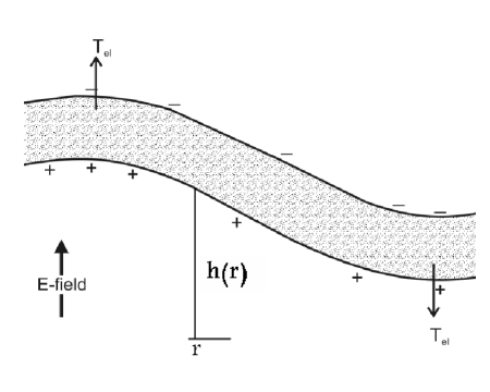
Figure 1: Net accumulation of conduction charges near a curved lipid membrane in an electric field, figure is based on ref [14]. T_el is the resulting normal stress component in the $z$-direction which enhances the local undulations h(r) of the membrane. It also induce a further surface tension in the membrane surface.

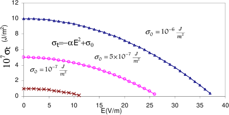
Figure 2: Total surface tension versus the electric field for three different values of $\sigma_{0}$.

The similarity of the equation (2) and the second term on the RHS of equation (1) is clear. Both represent the surface tension contributions to the Hamiltonian, one relating to the cytoskeleton-generated surface tension and the other only appears when an external electric field is applied.

For typical values of the parameters quoted in [14], one gets $\alpha=0.71\times 10^{-9}$ $\frac{J}{V^{2}}$. Therefore, the total membrane surface tension $\sigma_{t}$ (which appear in the surface tension part of the Hamiltonian) as the sum of electricaly induced part $\sigma_{el}$ and cytoskeleton-generated membrane surface tension $\sigma_{0}$ may be written as

$$\sigma_{t}=\sigma_{el}+\sigma_{0}.$$ (4)

The electric part of surface tension $\sigma_{el}$, being negative, enhances the undulations of the membrane while $\sigma_{0}$, the intramembrane tension, tends to keep the membrane surface unaltered. Note that we use positive values for $\sigma_{t}$ to satisfy the nearly-flat assumption. Typical values for the intramembrane tension and bending rigidity of a fluctuating membrane at room temperature for different lipid materials are $10^{-9}\frac{J}{m^{2}}\leq\sigma_{0}\leq 10^{-6}\frac{J}{m^{2}}$ [17] and $\kappa_{0}\sim 10^{-20}J$ ($\simeq 2.5k_{B}T$) [20], respectively. These values correspond to the following range of values for the electric field, using equation (3) and (4), presented in Table I.

$\sigma_{0}(\frac{J}{m^{2}})$	$E(\frac{V}{m})$
$10^{-6}$	$37.9$
$10^{-7}$	$12.0$
$10^{-8}$	$3.5$
$10^{-9}$	$1.2$

Table I: Upper bounds for the electric field corresponding to arbitrary intramembrane surface tension $\sigma_{0}$, used in the present work. As can be seen, the weaker the electric field, the lower the value of $\sigma_{0}$. A membrane with larger $\sigma_{0}$ can withstand higher electric fields.

The above values for the electric field have been taken with the view that the assumption of a nearly flat membrane is satisfied and is not violated by the application of too strong an electric field. They indicate that a membrane with weak surface tension is more affected by an electric field than a membrane with a stronger surface tension. Figure 2 shows variations of $\sigma_{t}$ with respect to the electric field for three values of $\sigma_{0}$.

2.2 The effective bending rigidity in an electric field

One can assume a similar equation for the total bending rigidity $\kappa_{t}$ as the sum of the electric contribution $\kappa_{el}$ and the cytoskeleton-generated rigidity $\kappa_{0}$, that is

$$\kappa_{t}=\kappa_{el}+\kappa_{0}.$$ (5)

In what follows, we will make an estimate of $\kappa_{el}$ using the theory of charged membranes and equation (4) and show that $\kappa_{el}$ is two order of magnitude smaller than $\kappa_{0}$ used below.

Let us assume that the membrane is charged due to the influence of an external electric field and the resulting accumulated net charge fluctuates on the surface. In such a scenario the contributions of $\sigma_{el}$ and $k_{el}$ to the surface tension and bending rigidity which stem from charge fluctuations, are both negative. In the limit of large membrane undulations, the following relation for the negative surface tension may be written [5]

$$\sigma_{el}=-\frac{\pi}{2\lambda^{2}}k_{B}T~{}\left[\frac{2\pi\lambda}{a}-\ln\left(1+\frac{2\pi\lambda}{a}\right)\right],$$ (6)

where $\lambda$ is a characteristic length similar to that of the Gouy-Chapman length especially in the presence of counterions around the membrane and $a$ is the molecular cut-off. The solution of the Poisson-Boltzmann equation for a simple charged surface in the presence of counterions would enable one to define a characteristic length which decreases when the surface charge density goes to higher values. In the present study the membrane is charged via the external electric field and is not flat. However, we have assumed that the situation is similar to the case of a charged surface when $\lambda\gg a$. In this limit, we may safely ignore the logarithm term in equation (6) against $2\pi\lambda/a$. Equations (3) and (6) then implicitly lead to an expression for the characteristic length, $\lambda$, mentioned earlier

$$\lambda\simeq\frac{k_{B}T}{\epsilon_{m}}{\left(\frac{\pi g_{m}}{gEd}\right)}^{2}.$$ (7)

As can be seen, an increasing electric field causes $\lambda$ to decrease as a result of the increasing charge density, leading to a highly charged membrane. Also, when $a\rightarrow 0$, one has $\lambda\rightarrow\infty$, showing that for a small molecular cut-off, the membrane becomes poorly charged and that in the presence of counterions, the charges do not accumulate near the membrane and often move freely in the solvent. On the other hand, if $\frac{g_{m}}{g}$ decreases or $\kappa_{m}$ increases, $\lambda$ increases, since there would be a concentration of charges on the boundaries. The direct dependence of $\lambda$ on temperature is clearly seen. The dependence of $\lambda$ on the electric field strength and membrane conductivity is shown in Fig. 3.

In the same manner, if we assume that the membrane is charged by the application of the electric field so that net charges on the membrane can fluctuate, in the long wavelength limit, the following expression for the reduced bending rigidity holds [5]

$$\kappa_{el}=-\frac{\pi}{32}k_{B}T\ln\left(\frac{L+2\pi\lambda}{a+2\pi\lambda}\right),$$ (8)

where $L$ is a typical membrane length taken as $40\,\mu\mbox{m}$ here. Figure 4 shows variation of $\kappa_{el}$ with the electric field and $g_{m}$ for $g=1\frac{S}{m}$, $a=2nm$, $T=300K$ and $\epsilon_{m}=2\epsilon_{0}$. Note that the membranes become more flexible for higher values of both the field strength and membrane conductivity. This flexibility decreases rapidly when the membrane conductivity is low and the electric field strength is weak. It should be emphasized that the theory explained above may also be used when other sources are present. It has been used to study membranes with excess surface charge density [5] by dividing the Hamiltonian into three terms, that is, electrostatic interaction, entropic contribution and elastic energy. The effects of ionic salts on bending rigidity around cell membranes and in particular of micron-sized vesicles are an interesting problem to look at in that the combined effects of the salt and electric field induce cylindrical deformations [21] on such vesicles.

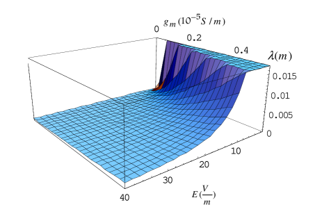
Figure 3: Variation of $\lambda$ in terms of different values of $E$ and $g_{m}$ for $g=1\frac{S}{m}$.

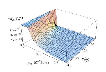
Figure 4: Variation of $-\kappa_{el}$ in terms of different values of $E$ and $g_{m}$ for $g=1\frac{S}{m}$.

The above discussions leads us, using equations (4) and (5), to write the Hamiltonian as

$${\cal H}=\frac{1}{2}\int d^{2}x\left\{\kappa_{t}(\nabla^{2}h)^{2}+\sigma_{t}(\nabla h)^{2}\right\}.$$ (9)

This form is particularly useful for deriving the height-height correlation function, from which the roughness associated with the membrane can be deduced.

3 The influence of an electric field on the roughness of lipid membranes

The study of roughness in lipid membranes is facilitated by treating the evolution of such a system in terms of stochastic processes. One way to introduce stochastic behavior into the dynamics of the membrane is to treat the height function, $h(x_{1},x_{2})$, as a stochastically fluctuating Wiener variable. This stochastic behavior can be communicated to the inclusions residing inside, and on the surface of the membrane. One may then proceed to obtain the height-height correlation function of the membrane in real space from which the roughness, associated with random changes in $h$, can be extracted. In the presence of an electric field and using the the Fourier representation of $h$, we arrived at the Hamiltonian [17]

$${\cal H}=\frac{1}{2}\int\frac{d^{2}q}{(2\pi)^{2}}\left\{\kappa_{t}q^{4}+\sigma_{t}q^{2}\right\}h({\bf q})h^{\ast}({\bf q})\,,$$ (10)

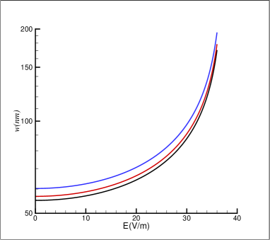
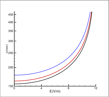
(a) (b)

Figure 5: Variation of the lipid membrane’s roughness versus the electric field for $L=40\mu m$, where $\sigma_{0}=10^{-6}\frac{J}{m^{2}}$ in the (a) panel and $\sigma_{0}=10^{-7}\frac{J}{m^{2}}$ in the (b) panel. In each panel $\kappa_{0}=10^{-20}(J),5\times 10^{-20}(J)$ and $10^{-19}(J)$ correspond to the top (blue), middle (red) and bottom (black) curves.

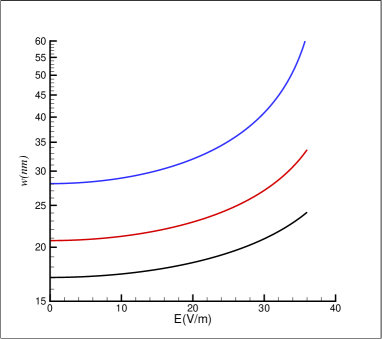
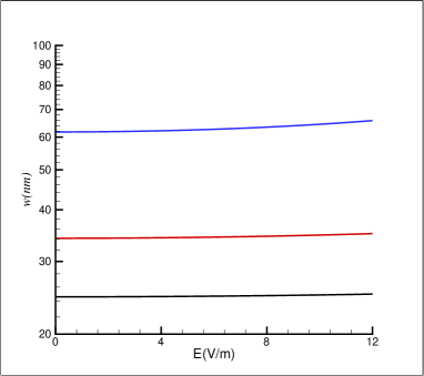
(a) (b)

Figure 6: Variation of the lipid membrane’s roughness versus the electric field for $L=500nm$, where $\sigma_{0}=10^{-6}\frac{J}{m^{2}}$ in the (a) panel and $\sigma_{0}=10^{-7}\frac{J}{m^{2}}$ in the (b) panel. In each panel $\kappa_{0}=10^{-20}(J),5\times 10^{-20}(J)$ and $10^{-19}(J)$ correspond to the top (blue), middle (red) and bottom (black) curves.

where $*$ denotes the complex conjugate. The static height-height correlation function can then be calculated as follows

$$\langle h({\bf q};0)h^{\ast}({\bf q^{\prime}};0)\rangle=\left(\frac{k_{\tiny\mbox{B}}T}{\kappa_{t}q^{4}+\sigma_{t}q^{2}}\right)(2\pi)^{2}\delta({\bf q}-{\bf q}^{\prime}).$$ (11)

The averaging is done with respect to the Boltzmann weight factor $\mbox{exp}(-\frac{\cal H}{k_{\tiny\mbox{B}}T})$, with $k_{\tiny\mbox{B}}$ being the Boltzmann constant. One can write the dynamic correlation function as [15]

$$h({\bf q};t)=h({\bf q};0)e^{-\gamma(q)t},$$

leading to

$$\langle h({\bf q};t)h^{\ast}({\bf q^{\prime}};0)\rangle=\left(\frac{k_{B}T~{}e^{-\gamma(q)t}}{\kappa_{t}q^{4}+\sigma_{t}q^{2}}\right)(2\pi)^{2}\delta({\bf q}-{\bf q}^{\prime}),$$ (12)

where $\gamma(q)$ is the damping factor reflecting the long-range character of the hydrodynamic damping given by

$$\gamma(q)=\frac{1}{4\eta}\left(\kappa_{t}q^{3}+\sigma_{t}q\right).$$ (13)

Let us now suppose that the fluid surrounding the membrane has a viscosity $\eta$. It is then possible to write the Fourier transform of (12) in real space (i.e, $\langle h({\bf x};t)h({\bf x};0)\rangle$), representing the dynamical mean roughness of the membrane as

$$w^{2}=\int\int\frac{d^{2}q}{(2\pi)^{2}}\frac{d^{2}q^{\prime}}{(2\pi)^{2}}\langle h({\bf q};t)h^{*}({\bf q^{\prime}};0)\rangle e^{-{\bf x}.({\bf q}-{\bf q^{\prime})}},$$ (14)

Substituting from (12) and (13) we find

$$w^{2}=\frac{1}{2\pi\beta}\int_{\frac{1}{L}}^{\frac{1}{a}}dq\frac{e^{-\frac{1}{4\eta}(\kappa_{t}q^{3}+\sigma_{t}q)t}}{\kappa_{t}q^{3}+\sigma_{t}q},$$ (15)

where $L$ is the linear size of the membrane and $a$ is the molecular cut-off, of the order of a nanometer, and $\beta=\frac{1}{k_{\tiny\mbox{B}}T}$. Here $t$ represents the correlation time [15] and is of the order of $10^{-4}s$ for the said values. Since there is no closed form expression for the integral given in equation (15), it should be computed by expanding the integrand as a series. The square root of $w^{2}$ is called root-mean-squared roughness (rms) when one assumes that $\langle h(x,t)\rangle=0$. Figure 5 and Fig. 6 demonstrate the variation of $w$ with respect to an electric field. We have limited the electric field values to those presented in Table I. Here, the three different values for the bending rigidity $\kappa_{0}=10^{-20}(J),5\times 10^{-20}(J)$ and $10^{-19}(J)$ correspond to the top, middle and bottom curves in each panel respectively. Note that in the (a) panels, $\sigma_{0}=10^{-6}\frac{J}{m^{2}}$ while in the (b) panels $\sigma_{0}=10^{-7}\frac{J}{m^{2}}$. Also the typical values have been used as $a=2nm$, $T=300K$, and $\eta=10^{-3}\frac{Js}{m^{3}}$.

Note that the dimension of roughness in the figures is nanometer. The following observations worth mentioning: that the roughness values are of the order of a few hundred nanometers and that the decrease in $\kappa_{0}$ and $\sigma_{0}$ and the increase in $L$ cause the roughness to increase. Here, it would be useful to mention that the observations of a typical membrane with $L=10\,\mu\mbox{m}$ by AFM have yielded a roughness in the range 12-70 nanometers [6]. Also, results from molecular dynamics and monte carlo simulations of lipid membranes with sizes of the order of nanometers [12] show that they experience a roughness of the order of a few angstroms. For stronger fields, we see a dramatic change in the roughness, starting roughly at $30\frac{V}{m}$ for $\sigma_{0}=10^{-6}\frac{J}{m^{2}}$ and $10\frac{V}{m}$ for $\sigma_{0}=10^{-7}\frac{J}{m^{2}}$. Therefore, the presence of an external electric field leads to the undulations or roughening of the membrane surface. Smaller values for correlation time lead to a lesser increase in rms roughness and vice versa.

4 Conclusions

In this paper we have studied the behavior of lipid membranes in the presence of an external electric field. The negative contribution to the surface tension as a result of the application of the field, the effects of an external electric field on the roughening of membranes and an estimation of the thickness of charges aggregated on the membrane surface were reviewed. The dependence of bending rigidity on electric fields and its relation to the thickness mentioned above was studied. The increase in the membrane rms roughness for larger electric field values was calculated and shown to contribute to the roughening of the membrane surface.

References

- [1] K. A. Riske and R. Dimova, Biophys. J. 88 (2005) 1143.
- [2] I. G. Abidor, V. B. Arakelyan, L. V. Chernomordik, Y. A. Chizmadzhev, V. F. Pastushenko, and M. R. Tarasevich, J. Electroanal. Chem. 104 (1979) 37.
- [3] D. Needham, and R. M. Hochmuth, Biophys. J. 55 (1989) 1001
- [4] H. G. L. Coster and T. C. Chilcott, Bioelectrochemistry 56 (2002) 141.
- [5] Y. W. Kim and W. Sung, Europhys. Lett. 58 (2002) 147.
- [6] E. M. V. Hoek, S. Bhattacharjee and M. Elmelech, Langmuir 19 (2003) 4836.
- [7] W. Richard Bowen and Teodora A. Doneva, J. Colloid Interface Sci. 229 (2000) 544.
- [8] S. V. Morozov, K. S. Novoselov, M. I. Katsnelson, F. Schedin, L. A. Ponomarenko, D. Jiang, and A. K. Geim, Phys. Rev. Lett. 97 (2006) 016801.
-
[9]
R. Lipowsky, Encyclopedia of Applied Physics,
23 (1998) 199,
R. Lipowsky, Current Opinion in Structural Biology 5, (1995) 531-540. - [10] P. Dietz, P. K. Hansma, O. Inacker, H. D Lehmann and K. H Herrmann, J. Membr. Sci. 65, (1992), 101.
- [11] Klaus-Peter Schneider, Chem. Phys. Lett 261 (1996) 1778.
- [12] Oded Farago, J. Chem. Phys 119 (2003) 596.
- [13] H. Isambert, Phys. Rev. Lett. 80 (1998) 3404.
- [14] P. Sens and H. Isambert, Phys. Rev. Lett. 88 (2002) 128102-1.
- [15] U. Seifert, Adv. in Phys. 46( 1997) 13.
- [16] H. Rafii-Tabar and H.R. Sepangi, Comp. Mat. Sci. 15 (1999) 483.
- [17] H. Rafii-Tabar and H. R. Sepangi, Physica A 357 (2005) 485.
- [18] P. B. Canham, J. Theor. Biol. 26 (1970) 61.
- [19] W. Helfrich, Z. Naturforsh, 28c (1973) 693.
- [20] M. Kummrow and W. Helfrich, Phys. Rev. A 44 (1991) 8356.
- [21] K. A. Riske and R. Dimova, Biophys. J. 91 (2006) 1778.