Abstract

We show how the entangled photons produced in parametric down conversion can be used to improve the sensitivity of a Sagnac interferometer. Two-photon and four-photon coincidences increases the sensitivity by a factor of two and four respectively. Our results apply to sources with arbitrary pumping and squeezing parameters.

OCIS codes: (120.3180) Interferometry; (270.4180) Multiphoton processes; (120.5790) Sagnac effect;

1 Introduction

When two electromagnetic waves counter-propagate along a circular path in rotation they experience different travel times to complete the path. This induces a phase shift between the two counter-propagating waves proportional to the angular velocity of the rotation. This phase difference is called as the Sagnac effect [1] and in addition to its scientific importance, it has numerous practical applications such as detection and high-precision measurement of rotation. It was studied and used in optics only with lasers until the new work [2] where they demonstrated the single-photon interference in the fiber Sagnac interferometer using spontaneous parametric down conversion as the source of single photons. However, it turns out that the results of interference are no different than with classical sources. This is also true of many interferometric experiments done at the single photon level [3, 4, 5]. Thus a natural question would be –what is the nature of interference if we replace the single photon source by entangled photon pair source. This is what we examine in detail. We find that the sensitivity of Sagnac interferometer could be considerably improved by using correlated photons [6, 7]. We thus bring Sagnac interferometer in the same class as other experiments on imaging [8, 9], lithography [10, 11, 12, 13, 14, 15] and spectroscopy [16].

Parametric down conversion (PDC) is predominant mechanism for experimentalists to create entangled photon pairs as well as single photons. Multi-photon entangled states produced in the down-conversion process is often used in quantum information experiments and applications like quantum cryptography and the Bell inequalities. In particular, demonstrations of two-photon [17, 18, 19, 20] and four-photon [21, 22] interferences are holding promise for realizable applications with entanglement-enhanced performance. The principle of this enhancement lies in the fact that “the photonic de Broglie wavelength” [23] of an ensemble of photons with wavelength $\lambda$ and number of photons $n$ can be measured to be $\lambda/n$ using a special interferometer. Further Steuernagel [24] has proposed the measurement of the reduced de Broglie wavelength of two- and four-photon wave packets.

In this paper we present an analysis of how parametric down converted photons could be useful to increase the rotation sensitivity in Sagnac interferometers. The results show two- and four-fold increase in the sensitivity which can be interpreted as a sign of two- and four-photon interference effect. The organization of the paper is as follows. The Sagnac ring interferometer is described in section 2 and the Sagnac phase shift is derived. In section 3, we analyze interference results with classical and quantum inputs. We compare the results obtained from entangled photon pairs input with classical and single-photon inputs. We show how the two-photon and four-photon coincidences increases the sensitivity in the phase shift. The visibility of the counts are also discussed. We conclude the paper in section 4 with a brief discussion on the disturbances that can effect the transmission of modes in fibers.

2 The Sagnac interferometer

The Sagnac interferometer consists of a ring cavity around which two laser light beams travel in opposite directions on a rotating base. One can form an interference pattern by extracting and heterodyning portions of the two counter-propagating beams to detect the rotation rate of the ring cavity relative to an inertial frame. The position of the interference fringes is dependent on angular velocity of the setup. This dependence is caused by the rotation effectively shortening the path distance of one beams, while lengthening the other. In 1926, a Sagnac interferometer has been used by Albert Michelson and Henry Gale to determine the angular velocity of the Earth. It can be used in navigation as a ring laser gyroscope, which is commonly found on fighter planes, navigation systems on commercial airliners, ships and spacecraft.

Fig. 1: Schematics of a Sagnac ring interferometer.

The Sagnac effect [1] can be understood by considering a circular ring interferometer like the one shown in Fig. 1. The input laser field enters the interferometer at point $P$ and split into clockwise (CW) and counterclockwise (CCW) propagating beams by a beam splitter. If the interferometer is not rotating, the beams recombine at point $P$ after a time given by

$$t=\frac{2\pi R}{c},$$ (1)

where $R$ is the radius of the circular beam path. However, if the interferometer is rotating with angular velocity $\Omega$, about an axis through the center and perpendicular to the plane of the interferometer, then the beams reencounter the beam splitter at different times. The transit times to complete one round trip for CW ($t_{2}$ at point $P_{2}$) and CCW ($t_{1}$ at point $P_{1}$) are given by,

$$t_{1}=\frac{2\pi R}{c+R\Omega}\,\,,$$ (2)

$$t_{2}=\frac{2\pi R}{c-R\Omega}\,\,.$$ (3)

Then one round trip time delay between the two beams is the difference

$$\Delta t=t_{2}-t_{1}=\frac{4\pi R^{2}\Omega}{c^{2}-R^{2}\Omega^{2}}\,\,.$$ (4)

For non-relativistic perimeter speeds (i.e. reasonable values of $R$ and $\Omega$), $R^{2}\Omega^{2}\ll c^{2}$, then

$$\Delta t=\frac{4\pi R^{2}\Omega}{c^{2}}\,\,.$$ (5)

The angular phase difference between the two counter propagating waves, the Sagnac effect, can be written as,

$$\phi=\omega\Delta t=\frac{8\pi}{\lambda\,c}A\Omega\,,$$ (6)

where $\lambda$ is the wavelength, $c$ the light velocity in vacuum, $A$ the interferometer area and $\Omega$ the angular velocity of the interferometer. A more general approach [26, 25, 27] shows that the phase shift does not depend on the shape of the interferometer and it is proportional to the flux of the rotation vector $\Omega$ through the interferometer enclosed area. Then one can increase the flux by using multi-turn round-trip path like utilizing an optical fiber. In terms of the total length of the optical fiber, $L$, we can recast Eq. (6) into

$$\phi=\frac{4\pi LR\Omega}{\lambda\,c}\,.$$ (7)

Eq. (7) shows that the phase shift induced by rotation of a Sagnac fiber ring interferometer increases linearly with the total length of the optical fiber.

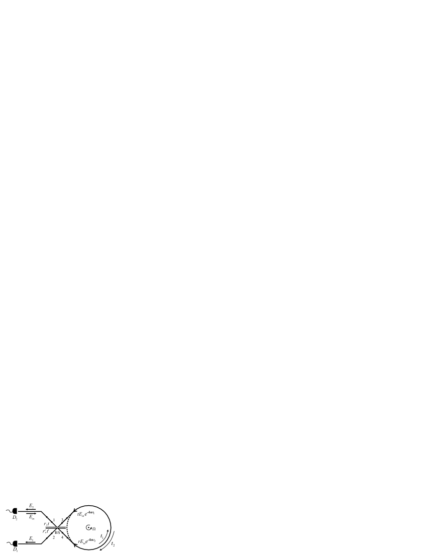
Fig. 2: The Sagnac interferometer setup with classical input. The input field $E_{in}$ is separated by the beam splitter into two counter-propagating waves $tE_{in}$ and $rE_{in}$. Because of the rotation they end up at the beam splitter at different times ($t_{1},t_{2}$).

3 The Sagnac interferometer with classical and quantum inputs

3.1 Classical input

We now consider a Sagnac fiber ring interferometer setup shown in Fig. 2. The two input ports 1 and 2 are mixed by a $50/50$ beam splitter and sent through a rotating loop of fiber in the opposite direction. Then the beams recombine at the beam splitter and come out from the ports they entered. The rotation induces the phase difference $\phi$ given by the Eq. (7). If we choose the transmission and reflection coefficients of the beam splitter as $t=1/\sqrt{2}=t^{\prime}$, $r=i/\sqrt{2}=r^{\prime}$ then the entire setup transforms the input field $E_{in}$ into the output fields $E_{1}$ and $E_{2}$ by

$$E_{1} = r^{\prime}rE_{in}e^{-i\omega t_{2}}+t^{2}E_{in}e^{-i\omega t_{1}}=E_{in}e^{-i\omega t_{2}}ie^{i\phi/2}\sin(\phi/2),$$ (8)

$$E_{2} = rtE_{in}e^{-i\omega t_{1}}+t^{\prime}rE_{in}e^{-i\omega t_{2}}=E_{in}e^{-i\omega t_{2}}ie^{i\phi/2}\cos(\phi/2),$$ (9)

where $\omega$ is the frequency of the input field. The intensity measurements at the detectors $D_{1}$ and $D_{2}$ becomes

$$I_{1} = |E_{1}|^{2}=|E_{in}|^{2}\sin^{2}(\phi/2),$$ (10)

$$I_{2} = |E_{2}|^{2}=|E_{in}|^{2}\cos^{2}(\phi/2),$$ (11)

respectively.

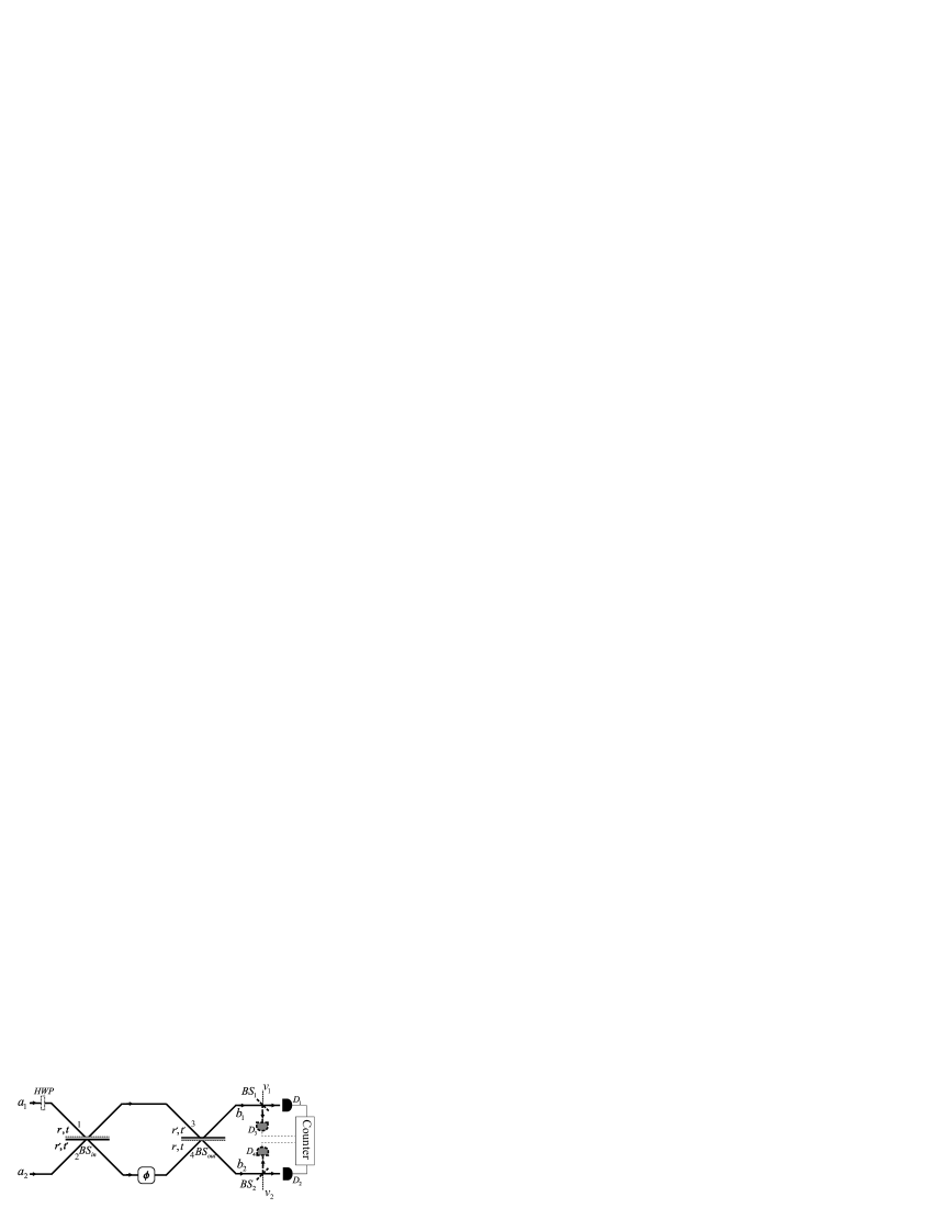
Fig. 3: The equivalent optical network diagram of the Sagnac interferometer for quantized fields. $``\,\phi\,"$ represents the phase shift provided by the rotating loop of the interferometer. The detectors $D_{3}$ and $D_{4}$ with the extra beam splitters (dashed lines) are to be used for four-photon coincidence counting.

3.2 Quantum inputs

Now we analyze the results with quantized fields. Figure 3 shows the equivalent optical network diagram of the interferometer. We denote $a_{1}$ and $a_{2}$ as the input mode operators. The two beam splitters represent double-use of the actual beam splitter. The output modes $b_{1}$ and $b_{2}$ are related to the input modes by

$$\left(\begin{array}[]{c}b_{1}\\ b_{2}\end{array}\right) = \underbrace{\frac{1}{\sqrt{2}}\left(\begin{array}[]{cc}1&i\\ i&1\end{array}\right)}_{BS_{out}}\underbrace{\left(\begin{array}[]{cc}1&0\\ 0&e^{i\phi}\end{array}\right)}_{SAGNAC}\underbrace{\frac{1}{\sqrt{2}}\left(\begin{array}[]{cc}1&i\\ i&1\end{array}\right)}_{BS_{in}}\left(\begin{array}[]{c}a_{1}\\ a_{2}\end{array}\right),$$ (22)

$$= ie^{i\phi/2}\left(\begin{array}[]{cc}-\sin(\phi/2)&\cos(\phi/2)\\ \cos(\phi/2)&\sin(\phi/2)\end{array}\right)\left(\begin{array}[]{c}a_{1}\\ a_{2}\end{array}\right),$$ (27)

where the global phase $ie^{i\phi/2}$ can be dropped. The use of half-wave plate ($HWP$) is required when the input ports have polarizations orthogonal to each other. Now the input and output modes are related to each other by the linear transformation,

$$b_{i}=\sum^{2}_{j=1}S_{ij}a_{j},$$ (28)

where the matrix $S$ of the coefficients $S_{ij}$ is known as the scattering matrix associated with the network. In fact, Eq. (28) refers to the Heisenberg picture, where the state vectors are constant while operators evolve. Therefore, without knowing the Hamiltonian that describes the evolution by the unitary operator $U$ on the state vectors, by using the dynamics of the operators

$$a_{i}\rightarrow b_{i}=\sum^{2}_{j=1}S_{ij}a_{j}\equiv U^{{\dagger}}a_{i}U,$$ (29)

$$a_{i}^{{\dagger}}\rightarrow b_{i}^{{\dagger}}=\sum^{2}_{j=1}S^{*}_{ij}a_{j}^{{\dagger}}\equiv U^{{\dagger}}a_{i}^{{\dagger}}U,$$ (30)

one can calculate the probabilities for detecting certain number of photons at certain outputs.

Now, let us analyze the rotation sensitivity to the phase shift $``\,\phi\,"$ for some Fock state inputs. We denote $n$-photons in mode $a_{1}$ and $m$-photons in mode $a_{2}$ by $|nm\rangle$. First, we begin with the input state $|10\rangle$, that is a single incident photon in mode $a_{1}$ with the other mode in vacuum state. The output state can be written as

$$U|10\rangle=Ua_{1}^{{\dagger}}|00\rangle=Ua_{1}^{{\dagger}}U^{{\dagger}}U|00\rangle=Ua_{1}^{{\dagger}}U^{{\dagger}}|00\rangle.$$ (31)

The last equality results from the fact that the interferometer has no effect on the vacuum $|00\rangle$. Although we are in the Schrödinger picture, it is perfectly valid to use Eq. (30) with the substitution $U\rightarrow U^{{\dagger}}\equiv U^{-1}$. This implies $S\rightarrow S^{{\dagger}}$ resulting

$$Ua_{i}^{{\dagger}}U^{{\dagger}}=\sum^{2}_{j=1}S_{ji}a_{j}^{{\dagger}}.$$ (32)

If we substitute Eq. (32) into Eq. (31) and use the scattering matrix given by Eq. (22), we find

$$U|10\rangle=-\sin(\phi/2)|10\rangle+\cos(\phi/2)|01\rangle,$$ (33)

up to an overall phase. Similarly we can calculate

$$U|11\rangle=\frac{1}{\sqrt{2}}\sin(\phi)(-|20\rangle+|02\rangle)+\cos(\phi)|11\rangle,$$ (34)

where the input is a pair of photons, one at each of the ports 1 and 2.

3.3 Single-photon input vs. two-photon input

The Heisenberg picture is convenient for computing the expectation values of photon numbers. For the single photon input $|10\rangle$, the intensities at the detectors $D_{1}$ and $D_{2}$ reads

$$I_{1}\equiv\langle b^{{\dagger}}_{1}b_{1}\rangle=\sin^{2}(\phi/2),$$ (35)

$$I_{2}\equiv\langle b^{{\dagger}}_{2}b_{2}\rangle=\cos^{2}(\phi/2),$$ (36)

whereas for the two-photon input $|11\rangle$, we have the single-photon counts at each detector $\langle b^{{\dagger}}_{1}b_{1}\rangle=1=\langle b^{{\dagger}}_{2}b_{2}\rangle$, i.e. there is no interference. On the other hand, by using Eq. (22), we can calculate the two-photon coincidences at the detectors $D_{1}$ and $D_{2}$,

$$I_{12}\equiv\langle b_{1}^{{\dagger}}b_{2}^{{\dagger}}b_{2}b_{1}\rangle=\cos^{2}(\phi),$$ (37)

which has twofold increase in the fringe pattern. This is also clear from the Schrödinger evolution of the state given by Eq. (34). The reason of this two-fold increase lies in the fact that when the two photons, one from each input port, enter into the loop, they transform into the following two-photon path-entangled state,

$$|11\rangle\rightarrow\frac{|20\rangle+|02\rangle}{\sqrt{2}}\rightarrow\frac{|20\rangle+e^{i2\phi}|02\rangle}{\sqrt{2}},$$ (38)

which shows a two-fold reduction in the wavelength of source photons. This was nicely demonstrated in the experiment [20] using photon pairs (biphotons) generated by spontaneous PDC.

3.4 Entangled photon pairs

We now discuss how the results given by Eqs. (10) and (11) are modified under conditions of arbitrary pumping, if we work with down-converted photons. To avoid coupling losses to a fiber, entangled photon pairs can also be generated inside a fiber at telecom wavelengths. This has been demonstrated by Kumar and coworkers [28]. The state produced in nondegenerate parametric down conversion can be written as

$$|\psi\rangle=\frac{1}{\cosh r}\sum_{n=0}^{\infty}(-e^{i\theta}\tanh r)^{n}|n\rangle_{1}|n\rangle_{2}.$$ (39)

This state can be generated mathematically by applying the two-mode squeeze operator $\hat{S}=\exp(\rho^{*}a_{1}a_{2}-\rho a_{1}^{{\dagger}}a_{2}^{{\dagger}})$ on vacuum, where $\rho=re^{i\theta}$ is the complex interaction parameter (also known as the squeezing parameter) proportional to the nonlinearity of the crystal, the pump amplitude and the crystal length. Polarization of photon pairs in the noncollinear type-I and the collinear type-II down-conversion are the same and orthogonal respectively. At first glance, it is easy to see that this state is nonseparable ($\equiv$ entangled) to a product of states of mode 1 and mode 2. It is already in Schmidt-decomposed form with a Schmidt number higher than 1 for $r>0$, which is a measure of entanglement [29]. Moreover one can calculate the Entropy of Entanglement [30], $E=-{\mathrm{T}r}_{2}\rho\log_{2}\rho$ as a function of $r$,

$$E=\cosh^{2}r\log_{2}(\cosh^{2}r)-\sinh^{2}r\log_{2}(\sinh^{2}r).$$ (40)

The amount of entanglement given by Eq. (40) is approximately linear in $r$ showing that the state in Eq. (39) is fully entangled for $r\rightarrow\infty$.

When the input modes are in the state given by the Eq. (39) the output detectors $D_{1}$ and $D_{2}$ read the single counts

$$I_{1}\equiv\langle b^{{\dagger}}_{1}b_{1}\rangle=\sinh^{2}r=\langle b^{{\dagger}}_{2}b_{2}\rangle\equiv I_{2},$$ (41)

which does not give any information on the rotation. On the other hand, the two-photon coincidence counts, after subtracting independent counts, normalized over the product of single counts at each detector becomes,

$$g^{2}_{12}=\frac{\langle b_{1}^{{\dagger}}b_{2}^{{\dagger}}b_{2}b_{1}\rangle}{\langle b^{{\dagger}}_{1}b_{1}\rangle\langle b^{{\dagger}}_{2}b_{2}\rangle}-1=\cos^{2}(\phi)\coth^{2}r,$$ (42)

which is twice more sensitive to the rotation than the result in Eq. (35) with 100% visibility. The signal itself depends on $r$ and it is most significant when $r\approx 1$. The regime with an interaction parameter value of $r=1.39$ has already been reached in the experiment [31].

On the other hand, we can employ a different measurement –the projective measurement,

$$P_{2} = {\mathrm{T}r}[|11\rangle\langle 11|\rho(\phi)]\equiv|\langle 11|U|\psi\rangle|^{2}$$ (43)

$$= \frac{\tanh^{2}r}{\cosh^{2}r}\cos^{2}(\phi),$$

which is the probability of detecting two photons, one at each detector operating in coincidence. Here the state $\rho(\phi)=U|\psi\rangle\langle\psi|U^{{\dagger}}$ is the evolved density matrix corresponding to the state given in Eq. (39). This probability can be easily calculated by utilizing the Schrödinger picture evolution of the state vector $|11\rangle$ given in Eq. (34). The expression in Eq. (43) is a pure two-photon interference effect showing by halving the de Broglie wavelength of the source photons. Thus, the two-photon coincidences by using the state in Eq. (39) shows two-fold increase in the sensitivity of the phase measurement.

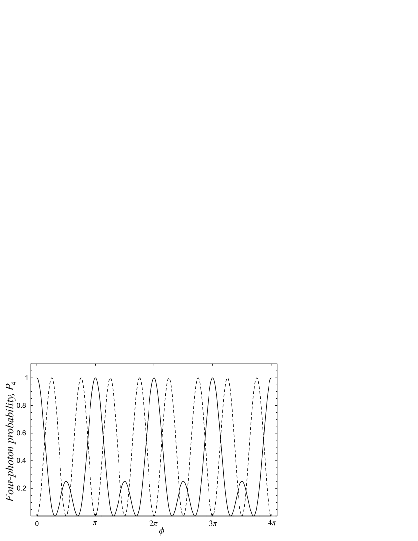
Fig. 4: Normalized four-photon probability in coincidence in 2-by-2 (solid line) and 3-by-1 (dashed line) detection scheme described by Eqs. (47) and (49) respectively.

The next question is– can we increase the sensitivity further by measuring higher order coincidences? We suggest employment of four single-photon detectors $D_{i}$ ($i=1,2,3,4$) as depicted in Fig. 3. We note that in a recent experiment [32] the tomography of the Fock state $|2\rangle$ was done by letting the two photons propagate in different directions and by single photon detectors. For detection of multi-photons, it is easier to use single photon detectors. We examine the coincidence of clicking four detectors i.e. the probability of the state $|1_{D_{1}}1_{D_{3}}1_{D_{2}}1_{D_{4}}\rangle$ where $D_{i}$’s denote the modes that goes into the corresponding detectors. This requires the state in modes $b_{1}$ and $b_{2}$ before the beam splitters $BS_{1}$ and $BS_{2}$ to be in a four-photon subspace. We now outline this calculation. The four-photon coincidence detection probability is given by

$$P_{4} = |\langle 1_{D_{1}}1_{D_{3}}1_{D_{2}}1_{D_{4}}|U_{B}U_{S}|\psi,0_{v_{1}}0_{v_{2}}\rangle|^{2}$$ (44)

$$= \langle 1_{D_{1}}1_{D_{3}}1_{D_{2}}1_{D_{4}}|U_{B}U_{S}|\psi,0_{v_{1}}0_{v_{2}}\rangle\langle\psi,0_{v_{1}}0_{v_{2}}|U_{S}^{{\dagger}}U_{B}^{{\dagger}}|1_{D_{1}}1_{D_{3}}1_{D_{2}}1_{D_{4}}\rangle,$$

where the state $|\psi,0_{v_{1}}0_{v_{2}}\rangle$ represents the tensor product of the state (39) with the vacuum ports $v_{1}$ and $v_{2}$ at the beam splitters $BS_{1}$ and $BS_{2}$. The unitary operators $U_{S}$ and $U_{B}$ represent the evolution of the states inside the Sagnac interferometer and the two beam splitters $BS_{1}$ and $BS_{2}$ respectively. First, we begin by calculating the inverse evolution

$$U_{B}^{{\dagger}}|1_{D_{1}}1_{D_{3}}1_{D_{2}}1_{D_{4}}\rangle = U_{B}^{{\dagger}}D_{1}^{{\dagger}}D_{3}^{{\dagger}}D_{2}^{{\dagger}}D_{4}^{{\dagger}}U_{B}U_{B}^{{\dagger}}|0000\rangle$$ (45)

$$= (t_{1}^{*}b_{1}^{{\dagger}}+r_{1}^{\prime*}v_{1}^{{\dagger}})(t_{2}^{*}b_{2}^{{\dagger}}+r_{2}^{\prime*}v_{2}^{{\dagger}})(r_{1}^{*}b_{1}^{{\dagger}}+t_{1}^{\prime*}v_{1}^{{\dagger}})(r_{2}^{*}b_{2}^{{\dagger}}+t_{2}^{\prime*}v_{2}^{{\dagger}})|0000\rangle$$

$$= t_{1}^{*}t_{2}^{*}r_{1}^{*}r_{2}^{*}b_{1}^{{\dagger}2}b_{2}^{{\dagger}2}|0000\rangle+\ldots,$$

where we take only four-photon state in modes $b_{1}$ and $b_{2}$ because other terms are irrelevant in our calculation. Here $t_{i}$’s and $r_{i}$’s are transmittance and reflectance coefficients of the beam splitter $BS_{i}$ ($i=1,2$). Next, we operate $U_{S}^{{\dagger}}$ on the resultant state above,

$$U_{S}^{{\dagger}}t_{1}^{*}t_{2}^{*}r_{1}^{*}r_{2}^{*}b_{1}^{{\dagger}2}b_{2}^{{\dagger}2}|0000\rangle = t_{1}^{*}t_{2}^{*}r_{1}^{*}r_{2}^{*}U_{S}^{{\dagger}}b_{1}^{{\dagger}2}b_{2}^{{\dagger}2}U_{S}U_{S}^{{\dagger}}|0000\rangle$$ (46)

$$= t_{1}^{*}t_{2}^{*}r_{1}^{*}r_{2}^{*}\left(-\sin(\phi/2)a_{1}^{{\dagger}}+\cos(\phi/2)a_{2}^{{\dagger}}\right)^{2}$$

$$\times \!\!\!\!\!\!\!\!\left(\cos(\phi/2)a_{1}^{{\dagger}}+\sin(\phi/2)a_{2}^{{\dagger}}\right)^{2}|0000\rangle$$

$$= \left(\frac{1}{2}\sin(\phi)(-a_{1}^{{\dagger}2}+a_{2}^{{\dagger}2})+\cos(\phi)a_{1}^{{\dagger}}a_{2}^{{\dagger}}\right)^{2}|0000\rangle$$

$$= \frac{1}{2}[1+3\cos(2\phi)]|2200\rangle+\ldots,$$

where we use the transformation given by Eq. (22) between the modes $a_{1}$, $a_{2}$ and $b_{1}$, $b_{2}$. In the last line of the Eq. (46) the first two modes are $a_{1}$ and $a_{2}$, while the last two modes are the vacuum modes of the beam splitters $BS_{1}$ and $BS_{2}$. In the last line of Eq. (46) we take only the state which has equal number of photons in modes $a_{1}$ and $a_{2}$ because the input state $|\psi\rangle$ is a pair photon state which is given in Eq. (39). Therefore the absolute square of the inner product of the resultant state given in the Eq. (46) with $|\psi,0_{v_{1}}0_{v_{2}}\rangle$ gives us the four-photon coincidence probability

$$P_{4}=\frac{\tanh^{4}r}{\cosh^{2}r}|t_{1}t_{2}r_{1}r_{2}|^{2}\frac{1}{4}[1+3\cos(2\phi)]^{2}.$$ (47)

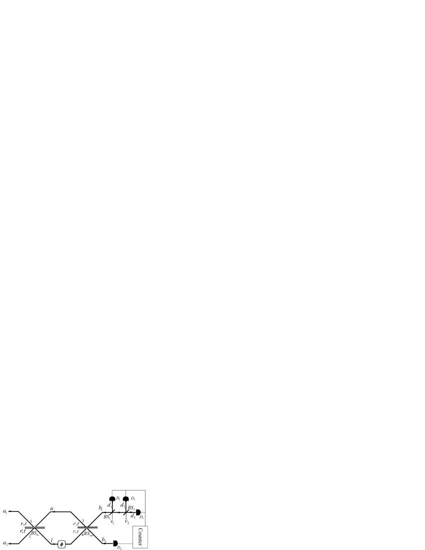
Fig. 5: The Sagnac interferometer setup for four-photon coincidence detection in 3-by-1 scheme.

The result given by Eq. (47) shows a reduction in the period of fringes by developing smaller peaks as depicted in Fig. 4. The phase sensitivity shows a four-fold increase w.r.t. the result in Eq. (35) obtained by single-photon input.

The four-photon coincidence detection can be done in an alternative way as depicted in figure 5. Here, three of the four photons are to be detected in the upper output channel $b_{1}$ while the fourth one goes into the detector placed in the lower output channel $b_{2}$. This time, we place the two extra beam splitters $BS_{1}$ and $BS_{2}$ to split up the three photons into single photons before they arrive at the detectors $D_{1}$, $D_{2}$ and $D_{3}$. Now, we begin with the evolution of the four-photon subspace term $|22\rangle$ provided by the input state $|\psi\rangle$,

$$|22\rangle = \frac{a_{1}^{{\dagger}2}}{\sqrt{2}}\frac{a_{2}^{{\dagger}2}}{\sqrt{2}}|00\rangle\,\,\longrightarrow\,\,\frac{1}{2}\left(\frac{iu^{{\dagger}}+l^{{\dagger}}}{\sqrt{2}}\right)^{2}\left(\frac{u^{{\dagger}}+il^{{\dagger}}}{\sqrt{2}}\right)^{2}|00\rangle$$ (48)

$$\longrightarrow -\frac{1}{8}\left\{\left(\frac{ib_{1}^{{\dagger}}+b_{2}^{{\dagger}}}{\sqrt{2}}\right)^{4}+e^{i4\phi}\left(\frac{b_{1}^{{\dagger}}+ib_{2}^{{\dagger}}}{\sqrt{2}}\right)^{4}+2e^{i2\phi}\left(\frac{ib_{1}^{{\dagger}}+b_{2}^{{\dagger}}}{\sqrt{2}}\right)^{2}\left(\frac{b_{1}^{{\dagger}}+ib_{2}^{{\dagger}}}{\sqrt{2}}\right)^{2}\right\}|00\rangle$$

$$= \frac{1}{4}\left\{e^{i2\phi}\sin(2\phi)b_{1}^{{\dagger}3}b_{2}^{{\dagger}}+\cdots\right\}|00\rangle$$

$$\longrightarrow \frac{e^{i2\phi}}{4}\sin(2\phi)\left\{\left(r_{1}d_{1}^{{\dagger}}+t_{1}(r_{2}d_{2}^{{\dagger}}+t_{2}d_{3}^{{\dagger}})\right)^{3}b_{2}^{{\dagger}}\right\}|0000\rangle$$

$$= \frac{e^{i2\phi}}{4}\sin(2\phi)\left\{6r_{1}t_{1}^{2}r_{2}t_{2}d_{1}^{{\dagger}}d_{2}^{{\dagger}}d_{3}^{{\dagger}}b_{2}^{{\dagger}}+\cdots\right\}|0000\rangle$$

$$= \frac{3}{2}e^{i2\phi}\sin(2\phi)r_{1}t_{1}^{2}r_{2}t_{2}|1111\rangle.$$

The arrow in the first line represents the evolution of the input modes into the interferometer after $BS_{in}$, while the second arrow shows further evolution of the modes by the phase shift $\phi$ and $BS_{out}$. In the third line we omit the terms giving photons in the channels other than three in $b_{1}$ and one in $b_{2}$. The fourth line shows how the channel $b_{1}$ split up into the modes $d_{1}$, $d_{2}$ and $d_{3}$ going into the detectors $D_{1}$, $D_{2}$ and $D_{3}$ respectively and since we are considering only one photon per detector we omit the other terms in the following line. In the last line we obtain the state corresponding to the four-photon coincidence detection in 3-by-1 scheme. Then, we calculate the probability of four-photon coincidence to be,

$$P_{4}^{(3by1)}=\frac{\tanh^{4}r}{\cosh^{2}r}|t_{1}^{2}t_{2}r_{1}r_{2}|^{2}\frac{9}{4}\sin^{2}(2\phi).$$ (49)

The normalized plot of this probability is shown in Fig. 4. Note that all the peaks are even in the interference pattern showing a pure four-fold increase in the sensitivity. We note that Steuernagel has a similar result in his work [24] on reduced de Broglie wavelength using precisely two photon events at each detector. In our proposal above we use single photon detectors to do four-photon coincidence. Currently efforts are on to find efficient nonlinear absorbers so that these could be used for detection of the precise number of photons [12, 33, 34].

4 Conclusion

There are advantages of using single photon interferometer as then the unwanted effects due to nonlinearities are avoided. However the integration time becomes long so that one can achieve the same level of sensitivity as classical interferometers [35]. What we are demonstrating is that we get superresolution relative to what is obtained by the usage of single photons. We think that experiments should be feasible because many two-photon and four-photon interference effects have been observed [17, 18, 19, 20, 21, 22].

There is one thing that should be in consideration in the use fiber. All fiber ring interferometers make use of single-mode fibers. Normally all single-mode fibers permit the transmission of modes of two orthogonal polarizations through the fiber in both directions. Disturbances, such as temperature fluctuations and mechanical stresses introduces birefringence to the fiber causing one mode to be transferred to the other. The noise produced by the transfer of modes from one to the other may effect the interference pattern. However by utilizing half-wave plates and polarization controllers [28] this noise may be suppressed.

We are grateful to NSF grant no CCF 0524673 for supporting this research.