Dirichlet or Potts ?

Abstract

When modeling the distribution of a set of data by a mixture of Gaussians, there are two possibilities:  i) the classical one is using a set of parameters which are the proportions, the means and the variances; ii) the second is to consider the proportions as the probabilities of a discrete valued hidden variable. In the first case a usual prior distribution for the proportions is the Dirichlet which accounts for the fact that they have to sum up to one. In the second case, to each data is associated a hidden variable for which we consider two possibilities: a) assuming those variables to be i.i.d. We show then that this scheme is equivalent to the classical mixture model with Dirichlet prior; b) assuming a Markovian structure. Then we choose the simplest markovian model which is the Potts distribution. As we will see this model is more appropriate for the case where the data represents the pixels of an image for which the hidden variables represent a segmentation of that image. The main object of this paper is to give some details on these models and different algorithms used for their simulation and the estimation of their parameters.
 
Key Words: Mixture of Gaussians, Dirichlet, Potts, Classification, Segmentation.

1 Introduction

When modeling the distribution of a set of data ${\mathb{x}}=\{x_{i},i=1,\cdots,N\}$ by a mixture of Gaussians (MoG), there are two possibilities:

• The classical one is using a set of parameters which are the proportions ${\boldsymbol{\alpha}}=\{\alpha_{k},k=1,\cdots,K\}$, the means ${\boldsymbol{\mu}}=\{\mu_{k},k=1,\cdots,K\}$ and the variances ${\mathb{v}}=\{v_{k},k=1,\cdots,K\}$:

  $$p(x)=\sum_{k=1}^{K}\alpha_{k}{\cal N}(x|\mu_{k},v_{k})$$ (1)

  and the objective is the estimation of $K$ and the parameters $\mathbb{\theta}=\{{\boldsymbol{\alpha}},{\boldsymbol{\mu}},{\mathb{v}}\}$.

• The second is to consider the proportions $\alpha_{k}$ as the probabilities of a discrete value hidden variable $Z$ whith $\alpha_{k}=P(Z=k)$:

  $$p(x)=\sum_{k=1}^{K}P(Z=k){\cal N}(x|\mu_{k},v_{k})$$ (2)

  which implies that $p(x|Z=k)={\cal N}(\mu_{k},v_{k})$.

In the first case a usual prior distribution for ${\boldsymbol{\alpha}}=\{\alpha_{k},k=1,\cdots,K\}$ is the Dirichlet

$${\mathcal{D}}({\boldsymbol{\alpha}}|{\boldsymbol{\lambda}})=\frac{\Gamma\left(\sum_{k}\lambda_{k}\right)}{\prod_{k}\Gamma(\lambda_{k})}\prod_{k=1}^{K}\alpha_{k}^{\lambda_{k}-1}$$ (3)

which accounts for the fact that $\sum_{k}\alpha_{k}=1$.

In the second case, to each data $x_{i}$ is associated a discrete value hidden variable $Z_{i}$. The value $z_{i}\in{1,\cdots,K}$ which takes $Z_{i}$ is then the class label of the datum $x_{i}$. When ${\mathb{x}}=\{x_{i},i=1,\cdots,N\}$ represent the pixels of an image, ${\mathb{z}}=\{z_{i},i=1,\cdots,N\}$ represents its segmentation. Then, naturally, we consider two possibilities for the distribution of ${\mathb{z}}$: a) assuming the variables $Z_{i}$ to be i.i.d.; b) assuming that there is a spatial structure through the image pixel index $i$ and thus assigning them a Potts Markov distribution.

In this paper we give some details on these models and different algorithms used for their simulation and the estimation of their parameters.

2 Maximum Likelihood and Bayesian approaches

In model (1), the classical maximum likelihood (ML) method assumes that the data ${\mathb{x}}=\{x_{i},i=1,\cdots,n\}$ are i.i.d samples from (1) and thus

$${\mathcal{L}}({\mathb{x}}|\mathbb{\theta},K)=\prod_{i}p(x_{i})=\prod_{i=1}^{n}\sum_{k=1}^{K}\alpha_{k}{\cal N}(x_{i}|\mu_{k},v_{k}).$$ (4)

Then, for a given $K$, the objective is the estimation of $\mathbb{\theta}=\{(\alpha_{k},\mu_{k},v_{k}),k=1,\cdots,K\}$ which is defined as

$$\widehat{\mathbb{\theta}}=\arg\max_{\mathbb{\theta}}\left\{{\mathcal{L}}({\mathb{x}}|\mathbb{\theta})\right\}$$ (5)

It is important to note that, the likelihood expression can become degenerate in the sense that it may become unbounded for particular set of parameters and data Snoussi01c . This makes the estimation of the parameters by this approach difficult. This is the reason for many authors to propose the penalized likelihood criteria to overcome this difficulty. The penalization term has the role to eliminate this degeneracy Champagnat95 ; Ridolfi00 ; Ciuperca03 .

In the Bayesian approach, one assigns priors $\pi(\mathbb{\theta})$, finds the expression of the posterior

$$p(\mathbb{\theta}|{\mathb{x}})\propto{\mathcal{L}}({\mathb{x}}|\mathbb{\theta})\;\pi(\mathbb{\theta})$$ (6)

and then, an estimate $\widehat{\mathbb{\theta}}$ is defined either as the MAP estimate:

$$\widehat{\mathbb{\theta}}=\arg\max_{\mathbb{\theta}}\left\{{\mathcal{L}}({\mathb{x}}|\mathbb{\theta})\;\pi(\mathbb{\theta})\right\}$$ (7)

or the posterior mean

$$\widehat{\mathbb{\theta}}=\int\mathbb{\theta}\;p(\mathbb{\theta}|{\mathb{x}})\mbox{~{}d}\mathbb{\theta}=\frac{\int\mathbb{\theta}\;{\mathcal{L}}({\mathb{x}}|\mathbb{\theta})\;\pi(\mathbb{\theta})\mbox{~{}d}\mathbb{\theta}}{\int{\mathcal{L}}({\mathb{x}}|\mathbb{\theta})\;\pi(\mathbb{\theta})\mbox{~{}d}\mathbb{\theta}}$$ (8)

The choice of the prior $\pi(\mathbb{\theta})$ in the Bayesian approach for the MoG model has been the subject of interest for many Bayesian authors through the entropic or conjugate priors. Both approaches result to the same prior, at least for the proportion parameters $\alpha_{k}$ which is the Dirichlet prior (3). The conjugate priors for the means are the Gaussians

$$\pi(\mu_{k})={\cal N}(\mu_{k}|\mu_{0},v_{0})$$ (9)

and for the variances are the Inverse Gamma (IG).

$$\pi(v_{k})={\mathcal{I}}{\mathcal{G}}(v_{k}|\alpha_{0},\beta_{0})$$ (10)

What is also interesting to note is that using the IG prior for the variances in the MAP estimate results exactly to the necessary penalization term in the ML approach which is needed to eliminate the degeneracy of the likelihood.

Computing the ML solution (5) or the MAP solution (7) can be done either directly or through an EM algorithm, but the PM solution (8) can not be obtained analytically and needs Monté Carlo (MC) algorithms. It is curious to note that, in the EM algorithm as well as in the MC sampling methods, one introduces the notion of hidden variables which is the subject of the second case modeling.

3 Separable (Dirichlet) and Markovian (Potts) models for the hidden variables

In model (2), to each data $x_{i}$ is associated a hidden variable $Z_{i}$ and the assumption is that the data $x_{i}$ is a sample from $p(x_{i}|Z_{i}=k)={\cal N}(x_{i}|\mu_{k},v_{k}),\forall i$ where the $Z_{i}$ can only take the values $k=1,\cdots,K$.

Then if we assume $Z_{i}$ to be independent and identically distributed (iid):

$$P(Z_{i}=k)=\alpha_{k},\forall i\quad\mbox{and}\quad P(Z_{i}=k,Z_{j}=l)=\alpha_{k}\alpha_{l},\forall i,j$$ (11)

we can write

$$P({\mathb{Z}}={\mathb{z}}|{\boldsymbol{\alpha}},K)=\prod_{i}\alpha_{z_{i}}=\prod_{k}\alpha_{k}^{\sum_{i}\delta(z_{i}-k)},$$ (12)

which means that ${\mathb{Z}}$ is separable in $Z_{i}$, then we can find a link between the two models (1) and (2) which become equivalent with $\alpha_{k}=\frac{1}{n}\sum_{i=1}^{n}\delta(z_{i}-k)$.

But if we assume that there are some structure (dependancy) in the hidden variables, then, we have to model them. The simplest model for such a structure is the Potts model:

$$P(Z_{i}=z_{i}|Z_{j}=z_{j},j\not=i)\propto\exp\left\{\gamma\sum_{j\in{\cal V}(i)}\delta(z_{i}-z_{j})\right\}$$ (13)

where ${\cal V}(i)$ represents the neighboring elements of $i$, for example ${\cal V}(i)=i-1$ or ${\cal V}(i)=\{i-1,i+1\}$ or in cases where $i$ represents the index of a pixel in an image, then ${\cal V}(i)$ represents the four nearest neigbors of that pixel. $\gamma$ is the Potts parameter.

Using the equivalence of Gibbs and Markovian distributions, we can also write

$$\left\{\begin{array}[]{lcl}\pi(z_{i}|z_{j},j\in{\cal V}(i),\gamma,K)&\propto&\exp\left\{\gamma\sum_{j\in{\cal V}(i)}\delta(z_{i}-z_{j})\right\}\\ \pi({\mathb{z}}|\gamma,K)&\propto&\exp\left\{\gamma\sum_{i}\sum_{j\in{\cal V}(i)}\delta(z_{i}-z_{j})\right\}\end{array}\right.$$ (14)

where $\pi(z_{i})$ stands in short for $P(Z_{i}=z_{i})$ and $\pi({\mathb{z}})$ stands in short for $P({\mathb{Z}}={\mathb{z}})$.

4 Data classification and Image segmentation

These two models have been used in many data classification or image segmentation where the $x_{i}$ represents either the grey level or the color components of the pixel $i$ and $z_{i}$ its class labels. The main objective of an image segmentation algorithm is the estimation of $z_{i}$. When the hyperparameters $K$, $\mathbb{\theta}=(\alpha_{k},\mu_{k},v_{k}),k=1,\cdots,K$ and $\gamma$ are not known and have also to be estimated, we say that we are in totally unsupervised mode, when are known we are in totally supervised mode and we say that we are in partially supervised mode when some of those hyperparameters are fixed. A classical case is the one with fixed $K$.

Assuming first $K$ known, we can write the following:

$$p({\mathb{x}}|{\mathb{z}},\mathbb{\theta},K)=\prod_{i\in{\mathcal{R}}}p(x_{i}|z_{i})=\prod_{i\in{\mathcal{R}}}{\cal N}(x_{i}|\mu_{z_{i}},\sigma_{z_{i}}^{2})=\prod_{k}\prod_{i\in{\mathcal{R}}_{k}}{\cal N}(x_{i}|\mu_{z_{i}},\sigma_{z_{i}}^{2})$$ (15)

where ${\mathcal{R}}=\{1,\cdots,n\}$ represents the set of all samples (all pixels positions of an image) and ${\mathcal{R}}_{k}=\{i:z_{i}=k\}$ represents the set of all samples who have the same label value $z_{i}=k$. Evidently, we assume that $\cup_{k}{\mathcal{R}}_{k}={\mathcal{R}}$ which means that all samples are classified.

$$p({\mathb{z}},\mathbb{\theta}|{\mathb{x}},K,\gamma)\propto p({\mathb{x}}|{\mathb{z}},\mathbb{\theta},K)\;\pi({\mathb{z}}|\gamma,K)\;\pi(\mathbb{\theta})$$ (16)

Then, one can try to estimate both ${\mathb{z}}$ and $\mathbb{\theta}$ from this expression either by alternate maximization:

$$\left\{\begin{array}[]{lcl}\widehat{{\mathb{z}}}&=&\arg\max_{{\mathb{z}}}\left\{p({\mathb{z}},\widehat{\mathbb{\theta}}|{\mathb{x}},K,\gamma)\right\}\\ \widehat{\mathbb{\theta}}&=&\arg\max_{\mathbb{\theta}}\left\{p(\widehat{{\mathb{z}}},\mathbb{\theta}|{\mathb{x}},K,\gamma)\right\}\end{array}\right.$$ (17)

or by first estimating $\theta$ and then using it for the estimation of ${\mathb{z}}$:

$$\widehat{\mathbb{\theta}}=\arg\max_{\mathbb{\theta}}\left\{p(\mathbb{\theta}|{\mathb{x}},K,\gamma)\right\}\longrightarrow\widehat{{\mathb{z}}}=\arg\max_{{\mathb{z}}}\left\{p({\mathb{z}}|\widehat{\mathbb{\theta}},{\mathb{x}},K,\gamma)\right\}.$$ (18)

However, the first step of this second approach cannot be done explicitly and needs an iterative algorithm using the hidden variables ${\mathb{z}}$ as the missing data. The Bayesian EM algorithm has particularly been developped for this:

$$\left\{\begin{array}[]{llcl}\mbox{E step:}&Q(\mathbb{\theta}|\widehat{\mathbb{\theta}}^{(t)})&=&\mbox{E}\left\{\ln p({\mathb{Z}},\mathbb{\theta}|{\mathb{x}},K,\gamma)|\widehat{\mathbb{\theta}}^{(t)}\right\}\\ \mbox{M step:}&\widehat{\mathbb{\theta}}^{(t+1)}&=&\arg\max_{\mathbb{\theta}}\left\{Q(\mathbb{\theta}|\widehat{\mathbb{\theta}}^{(t)})\right\}\end{array}\right.$$ (19)

The full Bayesian approach consists in exploring the whole posterior probability distribution by generating samples from it. This can be done through a Gibbs sampling algorithm:

$$\left\{\begin{array}[]{lcl}\widehat{{\mathb{z}}}&\sim&{p({\mathb{z}}|\widehat{\mathbb{\theta}},{\mathb{x}},K,\gamma)}\\ \widehat{\mathbb{\theta}}&\sim&{p(\mathbb{\theta}|\widehat{{\mathb{z}}},{\mathb{x}},K,\gamma)}\end{array}\right.$$ (20)

where

$$p({\mathb{z}}|\widehat{\mathbb{\theta}},{\mathb{x}},K,\gamma)\propto p({\mathb{x}}|\widehat{\mathbb{\theta}},{\mathb{z}},K,\gamma)\;\pi({\mathb{z}}|{\boldsymbol{\gamma}},K)$$ (21)

and

$$p(\mathbb{\theta}|\widehat{{\mathb{z}}},{\mathb{x}},K,\gamma)\propto p({\mathb{x}}|\widehat{\mathbb{\theta}},{\mathb{z}},K,{\boldsymbol{\gamma}})\;\pi(\mathbb{\theta})$$ (22)

where $\pi({\mathb{z}}|\gamma,K)$ is given either by (24) or by (25).

The main difficulty in these relations is that the joint distribution $p({\mathb{z}},\mathbb{\theta}|{\mathb{x}},K,\gamma)$ is not separable in its arguments. A framework which will give us the possibility to establish interesting relations between these approaches is the approximation of this joint distribution by a separable one which becomes variational techniques.

5 Variational Bayes

To be able to compare the two approaches, we consider

$$p({\mathb{z}},\mathbb{\theta}|{\mathb{x}},K)=p({\mathb{x}}|{\mathb{z}},\mathbb{\theta}_{1},K)\;\pi({\mathb{z}}|\mathbb{\theta}_{2},K)\;\pi(\mathbb{\theta}|K)/p({\mathb{x}}|K)$$ (23)

where $\mathbb{\theta}_{1}=\{{\boldsymbol{\mu}},{\mathb{v}}\}$, $\pi(\mathbb{\theta}_{1})=\pi({\boldsymbol{\mu}})\,\pi({\mathb{v}})=\sum_{k}\pi(\mu_{k})\,\pi(v_{k})$ with $\pi(\mu_{k})={\cal N}(\mu_{k}|\mu_{0},v_{0})$ and $\pi(v_{k})={\mathcal{I}}{\mathcal{G}}(v_{k}|\alpha_{0},\beta_{0})$ and where $\pi({\mathb{z}}|\mathbb{\theta}_{2},K)$ is given either by

$$\pi({\mathb{z}}|{\boldsymbol{\alpha}},K)=\prod_{i}P(Z_{i}=k|{\boldsymbol{\alpha}},K)=\prod_{k=1}^{K}\alpha_{k}^{\sum_{i}\delta(z_{i}-k)},$$ (24)

where $\mathbb{\theta}_{2}={\boldsymbol{\alpha}}$, or by

$$\pi({\mathb{z}}|\gamma,K)=\prod_{i}P(Z_{i}=k|{\mathb{z}}_{-i},{\boldsymbol{\alpha}},K)\propto\prod_{i}\exp\left\{\gamma\sum_{j\in{\cal V}(i)}\delta(z_{i}-z_{j})\right\}$$ (25)

where $\mathbb{\theta}_{2}=\gamma$ and where $\pi(\mathbb{\theta}|K)=\pi(\mathbb{\theta}_{1}|K)\;\pi(\mathbb{\theta}_{2}|K)$.

In these equations

$$p({\mathb{x}}|K)=\sum_{{\mathb{z}}}\int p({\mathb{x}},{\mathb{z}},\mathbb{\theta}|K)\mbox{~{}d}\mathbb{\theta}=\sum_{{\mathb{z}}}\int p({\mathb{x}}|{\mathb{z}},\mathbb{\theta}_{1},K)\;\pi({\mathb{z}}|\mathbb{\theta}_{2},K)\;\pi(\mathbb{\theta}|K)\mbox{~{}d}\mathbb{\theta}$$ (26)

which is the evidence of the model $K$ and can be used to determine $K$.

Let consider a free distribution $q({\mathb{z}},\mathbb{\theta})$ and compare it to the joint posterior $p({\mathb{z}},\mathbb{\theta}|{\mathb{x}},K)$ and the complete dat likelihood $p({\mathb{x}},{\mathb{z}},\mathbb{\theta}|K)$ via the the two following quantities:

• Free energy:

  $$\begin{array}[]{lcl}{\mathcal{F}}\left(q({\mathb{z}},\mathbb{\theta}):p({\mathb{x}},{\mathb{z}},\mathbb{\theta}|K)\right)&=&\sum_{{\mathb{z}}}\int q({\mathb{z}},\mathbb{\theta})\ln\frac{p({\mathb{x}},{\mathb{z}},\mathbb{\theta}|K)}{q({\mathb{z}},\mathbb{\theta})}\mbox{~{}d}\mathbb{\theta}\\ &=&\sum_{{\mathb{z}}}\int q({\mathb{z}},\mathbb{\theta})\ln\frac{p({\mathb{z}},\mathbb{\theta}|{\mathb{x}},K)\;p({\mathb{x}}|K)}{q({\mathb{z}},\mathbb{\theta})}\mbox{~{}d}\mathbb{\theta}\\ &=&\sum_{{\mathb{z}}}\int q({\mathb{z}},\mathbb{\theta})\ln\frac{p({\mathb{z}},\mathbb{\theta}|{\mathb{x}},K)}{q({\mathb{z}},\mathbb{\theta})}\mbox{~{}d}\mathbb{\theta}+\ln p({\mathb{x}}|K)\end{array}$$ (27)

• Kullback-Leibler relative entropy between the free distribution $q({\mathb{z}},\mathbb{\theta})$ and the joint posterior $p({\mathb{x}},{\mathb{z}}|\mathbb{\theta},K)$:

  $${\mathcal{K}}\left(q({\mathb{z}},\mathbb{\theta}):p({\mathb{x}},{\mathb{z}}|\mathbb{\theta},K)\right)=\sum_{{\mathb{z}}}\int q({\mathb{z}},\mathbb{\theta})\ln\frac{q({\mathb{z}},\mathbb{\theta})}{p({\mathb{z}},\mathbb{\theta}|{\mathb{x}},K)}\mbox{~{}d}\mathbb{\theta}$$ (28)

Then, we may note that

$$\ln p({\mathb{x}}|K)-{\mathcal{F}}\left(q({\mathb{z}},\mathbb{\theta}):p({\mathb{x}},{\mathb{z}},\mathbb{\theta}|K)\right)={\mathcal{K}}\left(q({\mathb{z}},\mathbb{\theta}):p({\mathb{x}},{\mathb{z}}|\mathbb{\theta},K)\right)\geq 0$$ (29)

so that the free energy ${\mathcal{F}}\left(q({\mathb{z}},\mathbb{\theta}):p({\mathb{x}},{\mathb{z}},\mathbb{\theta}|K)\right)$ is a lower bound for $\ln p({\mathb{x}}|K)$. This also shows that minimizing ${\mathcal{K}}\left(q({\mathb{z}},\mathbb{\theta}):p({\mathb{x}},{\mathb{z}}|\mathbb{\theta},K)\right)$ or maximizing ${\mathcal{F}}\left(q({\mathb{z}},\mathbb{\theta})\right)$ result to the same optimal solution $q({\mathb{z}},\mathbb{\theta})=p({\mathb{z}},\mathbb{\theta}|{\mathb{x}},K)$ which is the joint posterior.

These relations are valid for any $q({\mathb{z}},\mathbb{\theta})$ and in particular for a separable $q({\mathb{z}},\mathbb{\theta})=q_{1}({\mathb{z}})\;q_{2}(\mathbb{\theta})$. This remark is the main idea behind the variational Bayes method which tries to approximate the joint non-separable distribution $p({\mathb{z}},\mathbb{\theta}|{\mathb{x}},K)$ by a separable $q({\mathb{z}},\mathbb{\theta}|{\mathb{x}},K)=q_{1}({\mathb{z}})\;q_{2}(\mathbb{\theta})$ where $q_{1}$ and $q_{2}$ have to be determined in such a way that either the Kullback-Leibler criterion ${\mathcal{K}}(q:p)$ be minimized or the free energy ${\mathcal{F}}\left(q({\mathb{z}},\mathbb{\theta})\right)$ be maximized. Noting that

$$\begin{array}[]{lcl}{\mathcal{K}}\left(q_{1}({\mathb{z}})q_{2}(\mathbb{\theta}):p({\mathb{z}},\mathbb{\theta}|{\mathb{x}},K)\right)&=&\sum_{{\mathb{z}}}q_{1}({\mathb{z}})\left(\int q_{2}(\mathbb{\theta})\ln\frac{q_{2}(\mathbb{\theta})}{p({\mathb{z}},\mathbb{\theta}|{\mathb{x}},K)}\mbox{~{}d}\mathbb{\theta}\right)\\ &=&\sum_{{\mathb{z}}}q_{1}({\mathb{z}})\left(<p({\mathb{z}},\mathbb{\theta}|{\mathb{x}},K)>_{q_{2}(\mathbb{\theta})}-{\mathcal{H}}(q_{2})\right)\\ &=&\int q_{2}(\mathbb{\theta})\left(\sum_{{\mathb{z}}}q_{1}({\mathb{z}})\ln\frac{q_{1}({\mathb{z}})}{p({\mathb{z}},\mathbb{\theta}|{\mathb{x}},K)}\right)\mbox{~{}d}\mathbb{\theta}\\ &=&\int q_{2}(\mathbb{\theta})\left(<p({\mathb{z}},\mathbb{\theta}|{\mathb{x}},K)>_{q_{1}({\mathb{z}})}-{\mathcal{H}}(q_{1})\right)\end{array}$$

and the fact that ${\mathcal{K}}(q:p)$ is concave in $q_{1}$ for fixed $q_{2}$ and in $q_{2}$ for fixed $q_{1}$ its optimization can be done in an iterative way

$$\left\{\begin{array}[]{lclcl}\widehat{q}_{1}^{(t+1)}&=&\arg\min_{q_{1}}\left\{{\mathcal{K}}(q_{1}\;\widehat{q}_{2}^{(t)}:p)\right\}&=&\arg\max_{q_{1}}\left\{{\mathcal{F}}(q_{1}\;\widehat{q}_{2}^{(t)}:p)\right\}\\ \widehat{q}_{2}^{(t+1)}&=&\arg\min_{q_{2}}\left\{{\mathcal{K}}(\widehat{q}_{1}^{(t)}\;q_{2}:p)\right\}&=&\arg\max_{q_{2}}\left\{{\mathcal{F}}(\widehat{q}_{1}^{(t)}\;q_{2}:p)\right\}\end{array}\right.$$

where $t$ notes the iteration number. It is then easy to show that, at each iteration $t$, the solutions is obtained by computing the derivatives of the corresponding functionals and equating them to zero, which leads to:

$$\left\{\begin{array}[]{lcl}\widehat{q}_{1}^{(t+1)}({\mathb{z}})&\propto&\exp\left[{<\ln p({\mathb{x}},{\mathb{z}},{\boldsymbol{\Theta}}|K)>_{q_{2}^{(t)}(\mathbb{\theta})}}\right]\\ \widehat{q}_{2}^{(t+1)}(\mathbb{\theta})&\propto&\exp\left[{<\ln p({\mathb{x}},{\mathb{Z}},\mathbb{\theta}|K)>_{q_{1}^{(t)}({\mathb{z}})}}\right]\end{array}\right.$$ (30)

where $<.>_{q}$ mean the expectation over $q$. For more details on this approach see Dempster77 ; Ghahramani97 .

Noting that $p({\mathb{x}},{\mathb{z}},\mathbb{\theta}|K)=p({\mathb{x}}|{\mathb{z}},\mathbb{\theta},K)\,\pi({\mathb{z}}|\mathbb{\theta},K)\,\pi(\mathbb{\theta}|K)$, we see that the choice of the priors $\pi({\mathb{z}}|\mathbb{\theta},K)$ and $\pi(\mathbb{\theta}|K)$ as well as the choice of parametric family of $q_{1}({\mathb{z}})$ and $q_{2}(\mathbb{\theta})$ is of great importance for the expressions of $\widehat{q}_{1}^{(t+1)}({\mathb{z}})$ and $\widehat{q}_{2}^{(t+1)}(\mathbb{\theta})$ and their final $\widehat{q}_{1}^{*}({\mathb{z}})$ and $\widehat{q}_{2}^{*}(\mathbb{\theta})$. To obtain a computationally effective inference method, it is necessary to choose appropriately these distributions. For example, choosing conjugate priors for the hyperparameters $\pi(\mathbb{\theta}|K)$, we gain the advantage that the posterior $\pi(\mathbb{\theta}|{\mathb{z}},{\mathb{x}},K)$ or $\pi(\mathbb{\theta}|{\mathb{x}},K)$ expressions will be in the same family than the associated priors.

Between particular cases, we may mention the following:

Optimal case:  $q_{1}(z)=p({\mathb{z}}|{\mathb{x}},K)$  and  $q_{2}(\mathbb{\theta})=p(\mathbb{\theta}|{\mathb{x}},K)$
This means that $p({\mathb{z}},\mathbb{\theta}|{\mathb{x}},K)$ is approximated by the product $p({\mathb{z}}|{\mathb{x}},K)\,p(\mathbb{\theta}|{\mathb{x}},K)$. The solution in this case is immediate:

$$\left\{\begin{array}[]{l}\widehat{q}_{1}^{*}({\mathb{z}})=p({\mathb{z}}|{\mathb{x}},K)={\sum_{\mathb{z}}p({\mathb{x}}|{\mathb{z}},\mathbb{\theta},K)\,\pi({\mathb{z}}|\mathbb{\theta},K)}/{p({\mathb{x}}|K)}\\ \widehat{q}_{2}^{*}(\mathbb{\theta})=p(\mathbb{\theta}|{\mathb{x}},K)={\int p({\mathb{x}}|{\mathb{z}},\mathbb{\theta},K)\,\pi(\mathbb{\theta}|K)\mbox{~{}d}\mathbb{\theta}}/{p({\mathb{x}}|K)}\end{array}\right.$$

However, computing any of these two terms needs integration (integration over $\mathbb{\theta}$ for the first and summation over ${\mathb{z}}$ for the second.

Degenerate case:  $q_{1}({\mathb{z}})=p({\mathb{z}}|\widehat{\mathbb{\theta}}^{*},{\mathb{x}},K)$  and  $q_{1}(\mathbb{\theta})=p(\mathbb{\theta}|\widehat{{\mathb{z}}}^{*},{\mathb{x}},K)$.
where $\widehat{\mathbb{\theta}}^{*}$ and $\widehat{{\mathb{z}}}^{*}$ are two point estimators of $p(\mathbb{\theta}|{\mathb{z}},{\mathb{x}},K)$ and $p({\mathb{z}}|\mathbb{\theta},{\mathb{x}},K)$.
This case is obtained through the following iterations:

$$\left\{\begin{array}[]{l}\widehat{q}_{1}^{(t)}({\mathb{z}})=\delta({\mathb{z}}-\widehat{{\mathb{z}}}^{(t)})\\ \widehat{q}_{2}^{(t)}(\mathbb{\theta})=\delta(\mathbb{\theta}-\widehat{\mathbb{\theta}}^{(t)})\end{array}\right.\longrightarrow\left\{\begin{array}[]{l}\widehat{q}_{1}^{(t+1)}({\mathb{z}})=p({\mathb{z}}|\widehat{\mathbb{\theta}}^{(t)},{\mathb{x}},K)\\ \widehat{q}_{2}^{(t+1)}(\mathbb{\theta})=p(\mathbb{\theta}|\widehat{{\mathb{z}}}^{(t)},{\mathb{x}},K)\end{array}\right.$$

which means that $p({\mathb{z}},\mathbb{\theta}|{\mathb{x}},K)$ is approximated by the product $p({\mathb{z}}|\mathbb{\theta},{\mathb{x}},K)\,p(\mathbb{\theta}|{\mathb{z}},{\mathb{x}},K)$. Both expressions are available up to their normalizing factors:

$$\left\{\begin{array}[]{l}p({\mathb{z}}|\mathbb{\theta},{\mathb{x}},K)\propto p({\mathb{x}}|{\mathb{z}},\mathbb{\theta},K)\,\pi({\mathb{z}}|\mathbb{\theta},K)\\ p(\mathbb{\theta}|{\mathb{z}},{\mathb{x}},K)\propto p({\mathb{x}}|{\mathb{z}},\mathbb{\theta},K)\,\pi(\mathbb{\theta},K)\end{array}\right.$$

However, computing at each iteration $\widehat{\mathbb{\theta}}^{(t)}$ and $\widehat{{\mathb{z}}}^{(t)}$, which may be either the means or modes of these two distributions, may still need some effort. In particular, in the expression of $p({\mathb{z}}|\mathbb{\theta},{\mathb{x}},K)$, depending on the prior $\pi({\mathb{z}}|\mathbb{\theta},K)$ the computational cost and difficulties are different. The separable case of (24) is much easier than the Markovian case of (25).

Variational EM:
$q_{1}({\mathb{z}})=p({\mathb{z}}|\widehat{\mathbb{\theta}}^{*},{\mathb{x}},K)$  and  $q_{2}(\mathbb{\theta})=p(\mathbb{\theta}|{\mathb{x}},K)$  where  $\widehat{\mathbb{\theta}}^{*}=\arg\max_{\mathbb{\theta}}\left\{p(\mathbb{\theta}|{\mathb{x}},K)\right\}$.
This case is obtained through the following iterations:

$$\widehat{q}_{2}^{(t)}(\mathbb{\theta})=\delta(\mathbb{\theta}-\widehat{\mathbb{\theta}}^{(t)})\longrightarrow\left\{\begin{array}[]{ll}\widehat{q}_{1}^{(t+1)}({\mathb{z}})=p({\mathb{z}}|\widehat{\mathbb{\theta}}^{(t)},{\mathb{x}},K)\\ \widehat{\mathbb{\theta}}^{(t+1)}=\arg\max_{\mathbb{\theta}}\left\{Q(\mathbb{\theta},\widehat{\mathbb{\theta}}^{(t)})\right\}\mbox{~{}~{}with}&\mbox{(M step)}\\ Q(\mathbb{\theta},\widehat{\mathbb{\theta}}^{(t)})=<\ln p({\mathb{x}},{\mathb{Z}},\mathbb{\theta}|K)>_{p({\mathb{z}}|\widehat{\mathbb{\theta}}^{(t)},{\mathb{x}},K)}&\mbox{(E step)}\end{array}\right.$$

The next step in approximations is to choose $q_{1}({\mathb{z}})=\prod_{i}q_{1i}(z_{i})$ or $q_{2}(\mathbb{\theta})=\prod_{k}q_{2k}(\theta_{k})$ or both. The first case is only necessary for Markovian models of the labels.

Mean Field + EM:
$q_{1}({\mathb{z}})=\prod_{i}p(z_{i}|{\mathb{z}}_{-i},\widehat{\mathbb{\theta}}^{*},{\mathb{x}},K)$  and  $q_{2}(\mathbb{\theta})=p(\mathbb{\theta}|{\mathb{x}},K)$  where  $\widehat{\mathbb{\theta}}^{*}=\arg\max_{\mathbb{\theta}}\left\{p(\mathbb{\theta}|{\mathb{x}},K)\right\}$.

This case is obtained through the following iterations:

$$\left\{\begin{array}[]{l}q_{1}({\mathb{z}})=\prod_{i}q_{1j}(z_{i})\\ \widehat{q}_{2}^{(t)}(\mathbb{\theta})=\delta(\mathbb{\theta}-\widehat{\mathbb{\theta}}^{(t)})\end{array}\right.\longrightarrow\left\{\begin{array}[]{ll}\widehat{q}_{1j}^{(t+1)}(z_{i}|{\mathb{z}}_{-i})\propto p(z_{i}|{\mathb{z}}_{-i},\widehat{\mathbb{\theta}}^{(t)},{\mathb{x}},K)\\ \widehat{\mathbb{\theta}}^{(t+1)}=\arg\max_{\mathbb{\theta}}\left\{Q(\mathbb{\theta},\widehat{\mathbb{\theta}}^{(t)})\right\}\mbox{~{}~{}with}&\mbox{(M step)}\\ Q(\mathbb{\theta},\widehat{\mathbb{\theta}}^{(t)})=<\ln p({\mathb{x}},{\mathb{Z}},\mathbb{\theta}|K)>_{p({\mathb{z}}|\widehat{\mathbb{\theta}}^{(t)},{\mathb{x}},K)}&\mbox{(E step)}\end{array}\right.$$

where

$$p(z_{i}|{\mathb{z}}_{-i},\widehat{\mathbb{\theta}}^{(t)},{\mathb{x}},K)\propto p({\mathb{x}}|{\mathb{z}},\widehat{\mathbb{\theta}}^{(t)},K)\,p(z_{i}|{\mathb{z}}_{-i},\widehat{\mathbb{\theta}}^{(t)})$$

Mean Field + separable EM:
$q_{1}({\mathb{z}})=p({\mathb{z}}|\widehat{\mathbb{\theta}}^{*},{\mathb{x}},K)$  and  $q_{2}(\mathbb{\theta})=\prod_{k}q_{2k}(\mathbb{\theta}_{k}|{\mathb{x}},K)$  where  $\widehat{\mathbb{\theta}}_{k}^{*}=\arg\max_{\theta_{k}}\left\{p(\mathbb{\theta}_{k}|{\mathb{x}},K)\right\}$ where

$$\begin{array}[]{ll}q_{2}(\mathbb{\theta})=\prod_{k}q_{2k}(\alpha_{k})\,q_{2k}(\mu_{k})\,q_{2k}(v_{k})&\mbox{for Dirichlet}\\ q_{2}(\mathbb{\theta})=q_{2}(\gamma)\,\prod_{k}q_{2k}(\mu_{k})\,q_{2k}(v_{k})&\mbox{for Potts}\end{array}$$

Totally separable (Mean Field):
$q_{1}({\mathb{z}})=\prod_{i}p(z_{i}|{\mathb{z}}_{-i},\widehat{\mathbb{\theta}}^{*},{\mathb{x}},K)$  and  $q_{2}(\mathbb{\theta})=\prod_{k}q_{2k}(\alpha_{k})q_{2k}(\mu_{k})q_{2k}(v_{k})$.

6 Applications in data classification and in image segmentation

The mixture of Gaussians model are natural models for data classification. When the data are the scalar grey level $x_{i}$ or the color components ${\mathb{x}}_{i}$ of a pixel in an image, their classification result to the segmentation of that image. In the following, we note by ${\mathb{r}}_{i}$ the coordinate position of the pixel i, by $x_{i}=x({\mathb{r}}_{i})$ its grey level, by $z_{i}=z({\mathb{r}}_{i})$ its classification label and by ${\mathcal{R}}_{kl}=\{r_{i}:z({\mathb{r}}_{i})=k\}$ all the disjoint compact regions having the same label. We assume that ${\mathcal{R}}_{kl}\cap{\mathcal{R}}_{kl^{\prime}}=\phi$, ${\mathcal{R}}_{kl}\cap{\mathcal{R}}_{k^{\prime}l}=\phi$ and $\cup_{k}{\mathcal{R}}_{kl}\cap{\mathcal{R}}_{kl^{\prime}}={\mathcal{R}}$ which cover the whole image. What is more specifique in image segmentation compared to other data classification is the fact that there is a spatial organization of the data. A MoG model with Dirichlet prior does not account for this spatial organization, but the the same MoG with a Markovian Pottz prior accounts for that. There are also many other possibilities of modeling this spatial organization, but the Potts Markov model is the probably the simplest one. To illustrate this, let consider the image of the Figure 1-a and its original labels in b). The histogram of the image pixels c) is shown in c) and the histogram of the labels in d). The results of segmentation using MoG with Dirichlet prior are shown in e) supervised and in f) unsupervised. The results of segmentation using MoG with Potts prior are shown in g) supervised and in h) unsupervised. We observe that, in both cases of supervised and unsupervised, the results with Potts prior are better that those with Dirichlet priors.

.		.
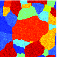
a) Original .	b) labels	c) histogram .	d) histogram
.		of image .	of labels
.		.
e) supervised .	f) unsupervised	g) supervised .	h) unsupervised
Dirichlet .	Dirichlet	Potts .	Potts
.		.
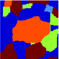
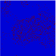
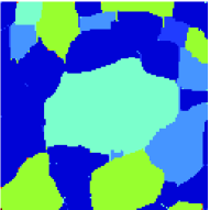
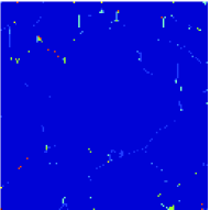
—e-b— .	—f-b—	—g-b— .	—h-b—
7.36% .	20.0%	1.83% .	4.64%

Figure 1: Classification and segmentation: a) an image, b) its original classification labels, c) histogram of the pixels, d) histogram of the labels, e) and f) Segmentation using MoG with Dirichlet (supervised and unsupervised; g) and h) Segmentation using MoG with Pottz (supervised and unsupervised); i,j,k,l are the classification errors (differences between original classification in b) and obtained classification in e), f), g) and h).

7 Conclusion

The mixture of Gaussians model are used extensively for data classification and in image segmentation. When there is no prior knowledge of any spatial organization of the data, the Dirichlet prior can be used. However, in image segmentation, this model often does not give satisfactory results, because the spatial organization of the pixels is ignored. Using the Potts prior gives better results because this prior accounts for the spatial organization of the pixels.