First season QUaD CMB temperature and polarization power spectra

Abstract

QUaD is a bolometric CMB polarimeter sited at the South Pole, operating at frequencies of 100 and 150 GHz. In this paper we report preliminary results from the first season of operation (austral winter 2005). All six CMB power spectra are presented derived as cross spectra between the 100 and 150 GHz maps using 67 days of observation in a low foreground region of approximately 60 square degrees. This data is a small fraction of the data acquired to date. The measured spectra are consistent with the $\Lambda$CDM cosmological model. We perform jackknife tests which indicate that the observed signal has negligible contamination from instrumental systematics. In addition by using a frequency jackknife we find no evidence for foreground contamination.

1. Introduction

The CMB is expected to be polarized at the $\sim 10\%$ level due to Thomson scattering by free electrons of the local quadrupole in the CMB radiation field at the time of last scattering. The resulting polarization signal can be decomposed into two independent modes. At the time of last scattering, even parity $E$-modes are generated by both scalar and tensor (gravitational wave) metric perturbations while odd-parity $B$-modes are generated only by gravitational waves. A secondary source of $B$-mode polarization comes from the weak gravitational lensing effect of intervening large scale structure, which converts $E$-modes into $B$-modes on small scales.

The first detection of the $E$-mode polarization signal was made by the 30 GHz radio interferometer, DASI, in 2002 (Kovac et al., 2002). Since then, in addition to a further measurement by the DASI experiment (Leitch et al., 2005), $E$-mode measurements have been made with the CBI (Readhead et al., 2004), CAPMAP (Barkats et al., 2005), BOOMERanG (Montroy et al., 2006), WMAP (Page et al., 2006) and MAXIPOL (Wu et al., 2006) experiments.

High precision measurements of the $E$-mode signal represent a non-trivial test of the standard cosmological model since the polarization of the CMB probes the velocity field at the time of last scattering, as opposed to the density field probed by CMB temperature measurements. In addition, accurate measurements of $E$-mode polarization can be useful for constraining certain cosmological parameters which are fairly insensitive to the CMB temperature field (e.g. isocurvature modes in the early Universe). Such a high resolution measurement of the $E$-mode polarization signal is the primary science goal of the QUaD experiment. In addition to the polarization, QUaD will, with further analysis, also provide interesting results on the CMB temperature field on small scales.

In this paper we present preliminary power spectra measured from QUaD’s first season of operation. The paper is organized as follows. In Section 2, we summarize the QUaD instrument and describe the observation strategy and low-level data reduction. Section 3 describes our map-making and simulation procedure. Our power spectrum estimation method is described in Section 4 and the power spectrum results are presented in Section 5 along with results from a number of jackknife tests. In Section 6 we estimate cosmological parameters using our spectra and our conclusions are presented in Section 7.

Throughout this paper when we refer to “the $\Lambda$CDM model” we mean specifically the model generated by the CMBFAST program (Zaldarriaga & Seljak, 2000) using the WMAP3 cosmological parameters given under the heading “Three Year Mean” in table 2 of Spergel et al. (2006). This is the model used in our simulations and shown in the plots.

2. Instrument Summary and Observations

QUaD is a millimeter-wavelength bolometric polarimeter designed for observing the CMB at two frequency bands, 100 and 150 GHz. The experiment is sited at the MAPO observatory, approximately 1 km from the geographic South Pole. First light was achieved in February 2005, and science observations began in May 2005. The telescope is a 2.6 m on-axis Cassegrain with nominal beam sizes of 6.3 (100 GHz) and 4.2 (150 GHz) arcminutes. The tower, ground shield and altitude-azimuth mount of the DASI experiment are re-used for QUaD, the ground shield being extended to accommodate the larger telescope structure. The mount has a third axis which rotates about the optical symmetry axis (termed “deck” rotation). This is a very useful feature for a polarimeter, as it allows the entire telescope to be rotated to an arbitrary angle with respect to the sky.

The QUaD receiver comprises two anti-reflection coated cryogenic re-imaging lenses and a focal plane array of 31 pixels, each composed of a corrugated feed horn and two orthogonal Polarization-Sensitive Bolometers (PSBs; Jones et al. (2003)). The PSB pairs are oriented on the focal plane in two groups with bolometer sensitivity angles separated by 45 degrees. This redundancy in detector orientation allows one to construct maps of the sky in Stokes $Q$ & $U$ with observations at a single deck angle if so desired. Each pixel is single-frequency and the pixels are divided between the two observing bands with 12 at 100 GHz and 19 at 150 GHz. The PSBs are similar to those flown on the successful B2K experiment (Masi et al., 2006). A complete description of the receiver along with details of the optical testing and characterization will be provided in Hinderks et al. (in prep).

The first season of QUaD observations were completed in October 2005 and consisted of $\sim$100 days of CMB runs, in addition to special runs for pointing model determination, beam mapping, and detector time constant measurements. The CMB runs consist of scanning the telescope back and forth by 7.5 degrees in azimuth, in a series of 30 second constant-elevation “half-scans”. The telescope is then stepped by 0.02 degrees in elevation and the process repeated to build up a raster map. Since the telescope is sited close to the Earth’s axis of rotation, azimuth and elevation closely approximate to right ascension and declination. In the first season we have mapped a 60 square degree patch in the low-foreground B2K deep region (Masi et al., 2006). For our chosen scanning speed and observing declination $\ell\sim 2000f$, where $f$ is the frequency in Hz at which multipole number $\ell$ appears in the time ordered data. The timeconstants of most (80%) of our detectors are less than 30 ms with the slowest two $\sim 100$ ms corresponding to half power roll-offs at $\ell\sim 10000$ and $\ell\sim 3000$ respectively.

To permit the removal of ground contamination, the scanning strategy employs a “lead-trail” scheme whereby each hour of observations is split equally between a “lead” field (1st half hour) and a “trail” field (2nd half hour), separated by 0.5 hours in right ascension. The lead and trail field observations follow exactly the same pattern in telescope azimuth and elevation so a constant ground signal can be removed by differencing the lead and trail field data. Furthermore, each day of observation is split into two 8 hour blocks made over different ranges in azimuth with the telescope rotated at different deck angles. This enables a powerful jackknife test as described below.

Initial processing of the raw time-ordered data (TOD) consists of glitch removal, deconvolution of the bolometer temporal response, low pass filtering and down-sampling. The relative calibration factor between channels (and within channels of a given pair) is derived from frequent short scans in elevation (el-nods) which introduce a strong atmospheric gradient into the TOD. This relative calibration is applied separately within each frequency group. Various quality control data cuts are applied at this stage: days with bad weather, bad pointing, poor focal plane temperature stability, or moon contamination are discarded. After applying these data cuts, 67 of the $\sim$100 days of CMB observations remain, and are used in the following science analysis.

3. Map-making and Simulation Process

Two analysis pipelines have been constructed which are independent in the sense that they share no code, although the algorithms are intended to be identical (with some important exceptions — see below). For this initial analysis we use data which has been point by point lead-trail differenced as described above. There is clear ground pickup in the data, which although mostly common mode, has a polarized component. This pickup appears to be completely canceled in the field difference. We note that many CMB experiments have mitigated ground pickup by field differencing, for example DASI.

Before mapping, a best-fit 3rd order polynomial is subtracted from each half-scan to remove the bulk of the $1/f$ noise. The signal from each PSB pair is then summed and differenced and co-added into the map according to the telescope pointing information. In the co-addition, a weighting is applied according to the inverse variance of each 30 second half-scan to properly account for differences in sensitivity across pairs, and to down weight periods of poorer weather. The pair sum data is used to construct total intensity ($T$) maps and the pair difference data is used to construct maps of Stokes $Q$ and $U$ by using the known orientation angle of each detector pair with respect to the sky. During this process, a $\sim 10\%$ correction for the non-ideal polarization efficiency is applied to the differenced PSB data. These angles and efficiencies are measured from special observations of a chopped, polarized, thermal source placed externally to the telescope.

While building the $T$, $Q$ and $U$ maps, we also construct the expected $T$, $Q$ and $U$ variance maps under the simple assumption that the noise is uncorrelated (white) in the TOD. These variance maps are used later to weight the signal maps in the power spectrum estimation stage.

As described in the next section the power spectrum estimation technique requires signal only, noise only, and signal plus noise simulations of the complete experiment. We generate these as follows.

To construct simulated noise timestreams, we Fourier transform each set of half-scans and take the auto and cross spectra between all channel pairs. This allows us to re-generate simulated noise timestreams with the same frequency spectra as the real data and the proper cross correlations between channels. We assume that the instantaneous signal to noise in the time-ordered data is sufficiently low that the power spectra created in this way accurately estimate the noise.

To generate simulated signal timestreams we generate realizations of $T$, $Q$ and $U$ sky maps under the $\Lambda$CDM model using the “synfast” generator (part of the HEALPix package), convolve with the instrumental beam (separately for each detector), and re-sample according to the pointing of the telescope. Included in this process are a scatter in the polarization efficiency factors of the PSB pairs and a scatter in the PSB sensitivity angles. The uncertainties used are derived from the special observations of a chopped, polarized thermal source mentioned above. A detailed beam model is used which is derived from special beam mapping runs on the compact HII region RCW38, daily scans of each detector across this source, and observations of a bright quasar PMN J0538-4405 which lies within our field.

Either of the signal or noise simulated timestream, or their sum, is then passed through the standard mapping algorithm (complete with polynomial subtraction and variance weighting) to yield simulated maps.

To derive the absolute calibration factor of our experiment we pass the B2K temperature maps (Masi et al., 2006) through the simulation process to provide maps which are filtered in exactly the same way as the QUaD maps, and are thus directly comparable to them. Both sets of maps are then Fourier transformed and cross spectra taken between them to determine the relative calibration factor. B2K is in turn calibrated against WMAP. (WMAP3 lacks sufficient sensitivity within our small sky area to allow a direct cross calibration.) We perform this calibration separately for the 100 GHz and 150 GHz maps, resulting in $5\%$ absolute calibration uncertainty in units of temperature ($10\%$ in units of power), including both QUaD and BOOMERanG uncertainties (Masi et al., 2006). To monitor the absolute stability of the instrument an internal calibration source is inserted into the beam frequently during routine data taking and these readings show excellent stability over the entire season of observations (few percent for any given channel and $0.5\%$ for the gain ratio of a PSB pair).

For visual presentation only, we divide by the variance map, transform to $E$ and $B$, and filter to the angular scales where signal to noise is highest, to produce Figure 1.

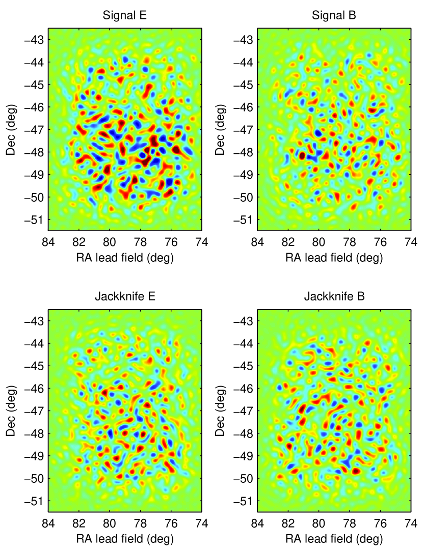
Figure 1.— QUaD first season field differenced polarization maps decomposed into $E$ and $B$-modes, and filtered to include only the angular scale range $200<\ell<1000$. The top row shows the result for signal (non-jackknife) maps, while the bottom row is for the “deck” jackknife (see text). This plot shows 150 GHz maps and the color scale is $\pm 30$ $\mu$K² in all cases.

4. Power Spectrum Estimation Method

To estimate angular power spectra, we employ a Monte Carlo (MC) based analysis. This method requires the creation of noise only simulated power spectra to correct the measured power spectra for noise bias, and signal only power spectra to allow the suppression of power by filtering to be corrected. In addition signal plus noise spectra are required to provide the final covariance matrix of the bandpower measurements.

Before measuring power spectra from the real and simulated maps, we apply an inverse variance mask to the maps based on the expected spatial distribution of the noise (using the variance maps mentioned above), and additionally mask a small number (5) of point sources which are apparent in our $T$ maps, and confirmed by external catalogs. We note that none of these sources is detected at high significance in the $Q$ and $U$ maps.

At this point the two pipelines diverge — one follows the standard MASTER technique of Hivon et al. (2002), extended to polarization (Brown et al., 2005), and works explicitly on the curved sky (pseudo-$C_{\ell}$), while the other makes the flat sky approximation and uses two dimensional Fourier transforms to derive power spectra.

The first pipeline measures raw pseudo-$C_{\ell}$ power spectra from the maps using a modified version of the “anafast” program included in the HEALPix package. Estimates of the CMB power spectra are then reconstructed as bandpowers (${\bf P}_{b}$) from the pseudo-$C_{\ell}$ measurements using

$${\bf P}_{b}=\sum_{b^{\prime}}{\bf M}^{-1}_{bb^{\prime}}\,\sum_{\ell}P_{b^{\prime}\ell}\,(\widetilde{\bf C}_{\ell}-\langle\widetilde{\bf N}_{\ell}\rangle_{MC}).$$ (1)

Here, $P_{b\ell}$ is a binning operator in $\ell$-space, $\widetilde{\bf C}_{\ell}$ are the raw pseudo-$C_{\ell}$ spectra measured from the real data and $\langle\widetilde{\bf N}_{\ell}\rangle_{MC}$ are the average pseudo spectra measured from the noise only simulations. ${\bf M}_{bb^{\prime}}$ is the binned coupling matrix of Brown et al. (2005) which corrects for mode-mixing due to the survey geometry. ${\bf M}_{bb^{\prime}}$ also contains the correction for the effects of both the TOD polynomial filtering and the telescope beam width. These corrections are derived from the set of signal only simulations. Finally, the covariance matrix of the resulting bandpowers is found from the scatter among the power spectra measured from simulations containing signal and noise.

The second pipeline takes the two dimensional Fourier transform of the masked maps, converts the $Q$ and $U$ Fourier modes into $E$ and $B$ and calculates bandpowers as the mean of the product of the modes within each annular bin. The product can be taken as the auto spectrum of a given map, or as a cross spectrum between two maps (which need not be at the same frequency). This is done for the real data maps and for each simulation realization. The data spectra then have the mean of the corresponding set of noise only simulations subtracted to noise correct them. Filter/beam suppression factors are calculated as the ratio of the mean of the signal only simulations to the input power spectra, and the data spectra are corrected by dividing out these suppression factors. Finally the bandpower covariance matrix is estimated from the scatter of the signal plus noise simulations in the same way as for pipeline one.

The first pipeline explicitly corrects for mixing between the $EE$ and $BB$ spectra due to the sky cut using the ${\bf M}_{bb^{\prime}}$ matrix. The second pipeline does not make such a correction, but the level of mixing into the $BB$ spectra in the signal only simulations is found to be negligible compared to the current instrumental sensitivity ($<0.2$ $\mu$K²). In addition note that the simulations indicate that inter- and intra-spectra mode mixing due to the half-scan polynomial filtering, and lack of cross linking in the map, are absolutely irrelevant for the current analysis.

For either pipeline we can take spectra internally within the sets of 100 and 150 GHz maps, or cross spectra between the two frequencies. In this paper, we present only the frequency cross spectra. The single frequency spectra will be presented in a future paper.

5. Results and Jackknife Tests

Figure 2 shows the frequency cross spectra measured from the first season of QUaD data by the two independent pipelines. The error bars are the square root of the diagonal elements of the bandpower covariance matrices which are estimated from the run-to-run scatter among MC simulations as described in the previous section. The first pipeline includes a mode decoupling step which narrows the $\ell$ range to which each bandpower responds, while at the same time changing the adjacent bandpower correlation coefficients from their “natural” value of $\approx+0.2$ to $\approx-0.2$. This leads to an increase in the diagonal of the bandpower covariance matrix which is reflected by larger error bars on the plot. However we emphasize that the total information content of the bandpowers from both pipelines is similar. In Figure 3 our results are shown compared to published results from other experiments.

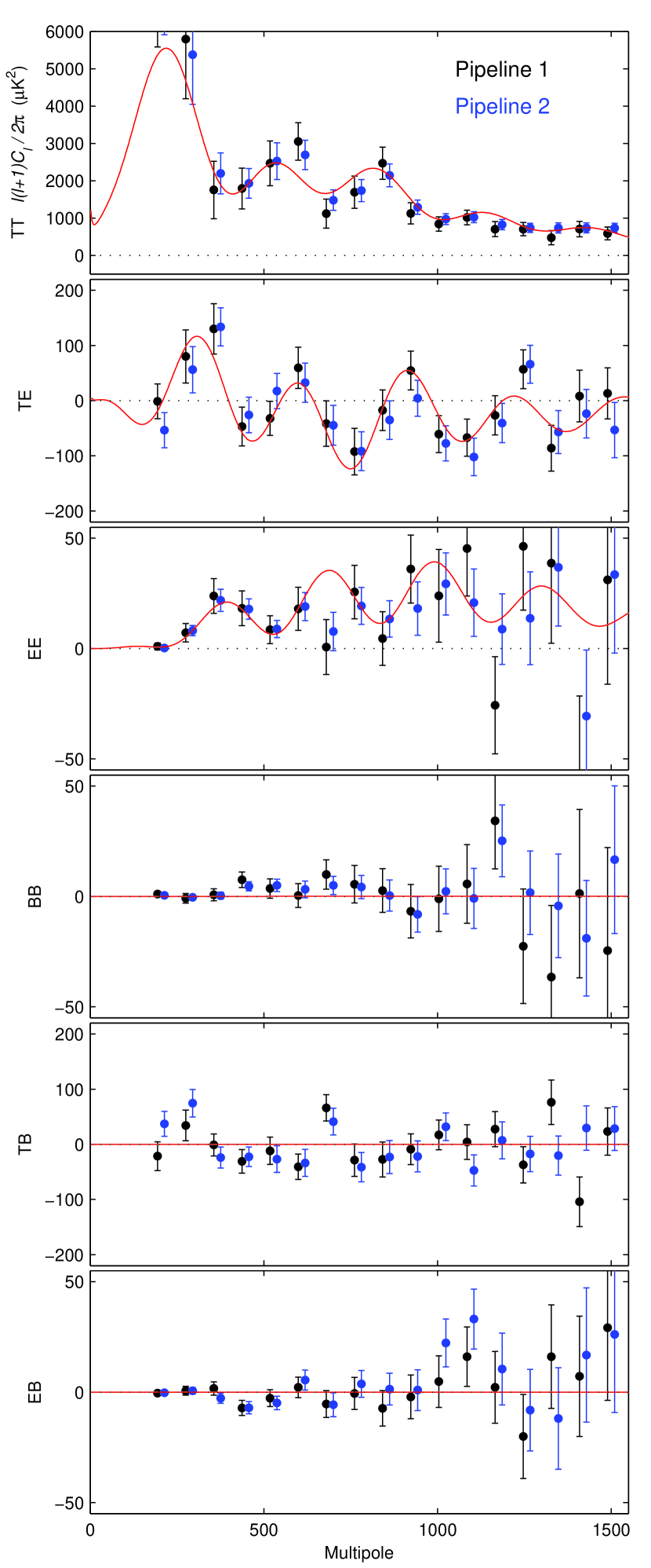
Figure 2.— Preliminary QUaD first season results derived as cross power spectra between the 100 and 150 GHz maps. The two sets of points are the results from two completely independent analyzes of the data (see text for details) and are displaced by $\pm 10$ in multipole number from their nominal values for clarity.

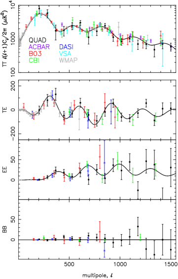
Figure 3.— Comparison of preliminary QUaD first season power spectrum results to selected other published results to date. The experiments compared to are ACBAR (Kuo et al., 2006), BOOMERanG (Jones et al., 2006; Piacentini et al., 2006; Montroy et al., 2006), CBI (Sievers et al., 2005), DASI (Leitch et al., 2005), VSA (Dickinson et al., 2004) and WMAP (Hinshaw et al., 2006; Page et al., 2006). Note that the $TT$ comparison is plotted with a log scale in the y-axis.

A powerful test for systematic contamination from ground pickup, or another source, is the so-called jackknife test. In this paper we use a map based jackknife, forming separate maps from various approximately equally sized data subsets, subtracting these and taking the power spectra of the result. We also do this for the signal plus noise simulations to estimate the expected uncertainty of the jackknife spectra. In as much as the signal originates on the sky it should exactly cancel under jackknife — depending on the split, and its origin, false signal is not likely to do so. Here we use the following data splits each of which will be explained in turn: deck split, scan direction split, season split, focal plane split and frequency split.

The so called deck split is possibly the most powerful test. As mentioned above each day of observations on our CMB field is split into two 8 hour blocks. Because the run starts always at the same local sidereal time these blocks occur always over the same range of azimuth angle as the telescope turns within its ground shield. In addition each block of observations is made always at the same rotation angle of the telescope with respect to the line of sight, with a 60 degree rotation occurring between the two blocks. Hence each given bolometer pair scans the sky at a different orientation angle within each block. Therefore the deck jackknife polarization maps will only cancel if the rotation to the absolute reference frame which occurs in the map making step is being performed correctly. The ground pickup is observed to be very complex with certain pair differences showing a detectable spike always at a certain azimuth angle and rotation angle of the telescope. Hence even if some ground pickup is leaking through the field differencing operation, we certainly do not expect it to appear identically in the deck split $Q$ and $U$ maps and thus to cancel in the deck jackknife. Figure 4 compares the signal (non-jackknife) and deck jackknife power spectra and we see that the vast majority of the apparent sky signal cancels. Note that where the signal spectra are sample variance dominated the jackknife spectra error bars are smaller since there is no sample variance in a null spectrum.

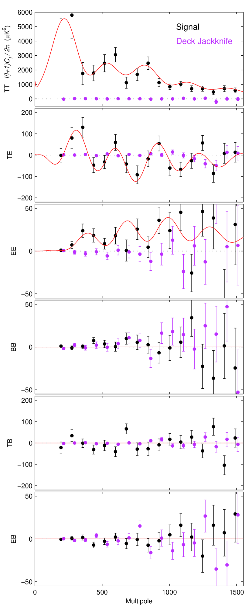
Figure 4.— QUaD signal spectra compared to deck jackknife spectra. (See text for details.)

For the scan direction jackknife we form separate maps from the half-scans in each direction. If deconvolution of the detector temporal response is not done correctly then the forward and backward maps will not match and residuals will remain when they are subtracted. In some cases the time constants of the two halves of a detector pair are not well matched and hence poor deconvolution could lead to leakage from $T$ into polarization making this a very important test.

The split season jackknife forms maps from the first half and second half of the used days. If for example there were a drift in the absolute calibration of the instrument over time then cancellation failure would be expected here.

The focal plane split forms separate maps using the two orientation groups of bolometer pairs in the focal plane. Because observations are taken at two deck angles it is possible to construct $Q$ and $U$ maps using each group.

For the frequency jackknife instead of taking cross spectra between the 100 GHz and 150 GHz maps we subtract them and take the spectra of the frequency difference maps. Any admixture of two or more signal components with differing spatial distributions and frequency spectral indexes is expected to fail this test (for example CMB plus synchrotron and/or dust) — this is therefore a stringent test for foreground contamination. Figure 5 compares the signal (non-jackknife) and frequency jackknife power spectra and we see that to the limits of experimental sensitivity the sky pattern is identical at the two frequencies.

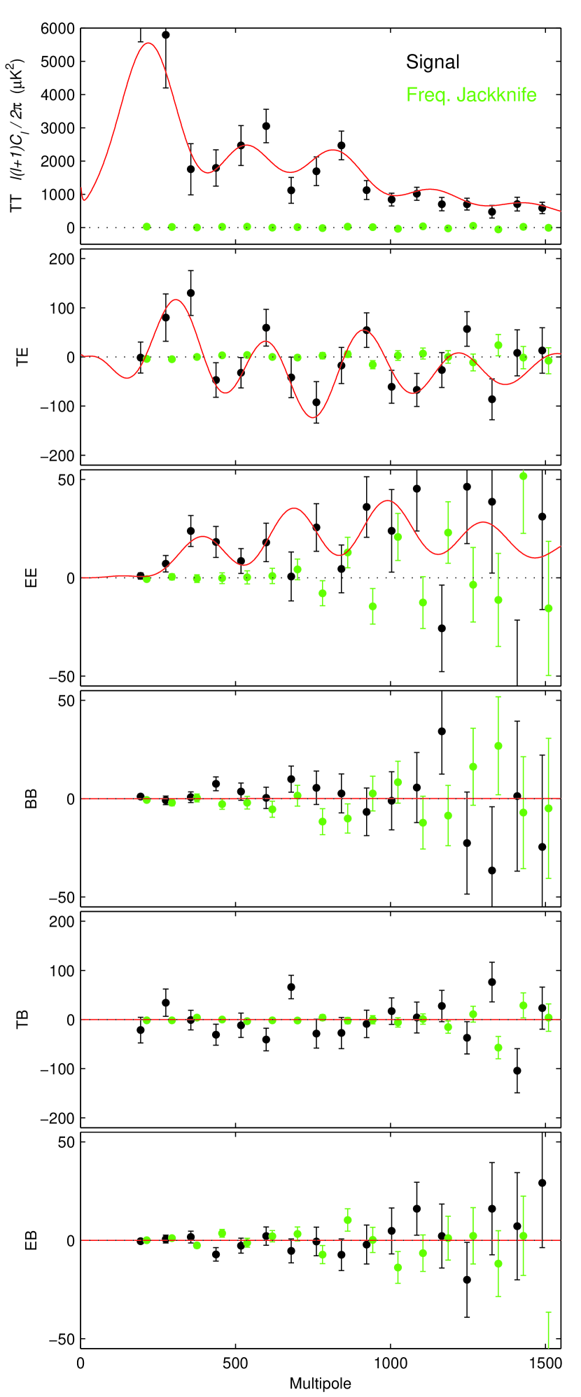
Figure 5.— QUaD signal spectra compared to frequency jackknife spectra. (See text for details.)

Figures 4 and 5 are visually impressive but to quantify how well these tests are passed we have calculated $\chi^{2}$ statistics for the comparison of the jackknife power spectra with the null model. For some of the jackknifes we do not expect perfect cancellation due to the interaction of the polynomial filtering by the half-scan and the non perfectly overlapping coverage region of the two data subsets. Hence we compare the measured $\chi^{2}$ values to the distribution which we measure from the set of signal plus noise simulations rather than to a theoretical $\chi^{2}$ distribution.

In Table 1, the probability to exceed (PTE) the $\chi^{2}$ value measured from the data is tabulated for each spectrum and jackknife test. These numbers are for the first pipeline — the second pipeline gives results which are similar. Ideally these PTE values should be uniformly distributed from zero to one. The only value which shows an obvious problem is $TT$ in the scan direction case — the enormous signal to noise of the $TT$ spectrum seen in Figures 4 and 5 makes the $TT$ jackknifes sensitive to tiny systematic errors. The jackknife tests of the single frequency spectra show some additional problems passing these formal $\chi^{2}$ tests and we are hence choosing not to publish these spectra at this time.

The final row of Table 1 is not a jackknife — it is a comparison of our measured spectra against the WMAP3 $\Lambda$CDM model mentioned above and shown in the plots. The PTE values lie within the acceptable range indicating that our measured spectra are consistent with this model.

Table 1PTE values from $\chi^{2}$ tests

Jackknife	$TT$	$TE$	$EE$	$BB$	$TB$	$EB$
Deck angle	0.236	0.208	0.812	0.435	0.274	0.062
Scan direction	0.000	0.173	0.304	0.375	0.236	0.223
Split season	0.032	0.814	0.257	0.527	0.904	0.111
Focal plane	0.193	0.702	0.079	0.503	0.450	0.225
Frequency	0.034	0.306	0.610	0.452	0.642	0.135
Signal	0.501	0.964	0.415	0.482	0.066	0.809

6. Cosmological Parameter Estimation

We have carried out a basic 6 parameter cosmological parameter constraint analysis using our polarization power spectra only, i.e. we use the $TE$, $EE$ and $BB$ spectra, but not $TT$. Our methodology uses the Monte-Carlo Markov Chain (MCMC) method and is based on that of the WMAP team as described in Verde et al. (2003); we impose the same flat priors, the same re-parameterization and the same convergence/mixing test. In addition we optimize the Markov chain step size choice, a fundamental parameter for the correct behavior of the algorithm, by calculating the parameter covariance matrix of a preliminary run of our chains as in Tegmark et al. (2004). We deal with the beam and calibration uncertainty using a method proposed by Bridle et al. (2002) which accomplishes an effective marginalization over these parameters by adding extra terms to the bandpower covariance matrix.

The theoretical power spectra are calculated using CAMB (Lewis et al., 2000), and then transformed by means of the experimental bandpower window functions to predictions for the binned $P_{b}$’s. We assume that the likelihood distribution for our bandpowers is Gaussian, which our signal plus noise simulations indicate is a valid assumption. The bandpower covariance matrix for the $P_{b}$’s is assumed to be independent of the model, and is estimated from the signal plus noise simulations as described above.

In Table 2 we present the marginalized expectation values and 68% confidence limits for each parameter. Four converged MCMC chains with around 50,000 steps each are merged to obtain these results. For all of the parameters our 68% confidence limit encloses the WMAP3 expectation value. The $\chi^{2}$ of the model with the parameters listed in the table is 44.1 giving a probability to exceed this by chance of 0.51 (for the 45 degrees of freedom).

Table 2 Polarization only cosmological parameter constraints using preliminary QUaD first season power spectra

Parameter	Symbol	Value
Baryon density	$\Omega_{b}h^{2}$	$0.0260\,\,_{-0.0059}^{+0.0061}$
Matter density	$\Omega_{m}h^{2}$	$0.142\,\,_{-0.031}^{+0.029}$
Hubble constant	$h$	$0.74\,\,_{-0.15}^{+0.16}$
Optical depth	$\tau$	$0.156\,\,_{-0.088}^{+0.089}$
Scalar fluctuation amplitude	$A_{s}$	$0.78\,\,_{-0.16}^{+0.16}$
Scalar fluctuation index	$n_{s}$	$0.833\,\,_{-0.293}^{+0.283}$

7. Conclusions

We have presented preliminary power spectra measured from the first season of observations with QUaD. In this paper we have presented only the frequency cross spectra taken between the 100 and 150 GHz maps. We find that these spectra are entirely consistent with the $\Lambda$CDM model — the measured $EE$ spectrum has a distinctive peak at $\ell\sim 400$ exactly as expected, the $TE$ spectrum shows the expected correlations, and the $BB$ spectrum is consistent with zero. A basic polarization only parameter constraint analysis yields confidence limits which agree with the WMAP3 results, and are as tight as those which were derived from CMB temperature spectra just a few years ago.

We have performed jackknife tests by measuring power spectra from differenced maps generated under several data splits and find that the results are free from significant instrumental systematics. In addition we have presented a frequency jackknife which indicates that contamination of the CMB by astrophysical foregrounds is negligible for the current experimental sensitivity.

We note that this analysis considers only frequency cross spectra and includes only 67 days out of a total of 250 days of CMB observing to date.

The QUaD experiment has begun a third season of observations and analysis of the second season data is underway. When completed, we fully expect to improve substantially on the preliminary results presented here.

References

- Barkats et al. (2005) Barkats, D. et al. 2005, ApJ, 619, L127, astro-ph/0409380
- Bridle et al. (2002) Bridle, S. L., Crittenden, R., Melchiorri, A., Hobson, M. P., Kneissl, R., & Lasenby, A. N. 2002, MNRAS, 335, 1193, astro-ph/0112114
- Brown et al. (2005) Brown, M. L., Castro, P. G., & Taylor, A. N. 2005, MNRAS, 360, 1262, astro-ph/0410394
- Dickinson et al. (2004) Dickinson, C. et al. 2004, MNRAS, 353, 732, arXiv:astro-ph/0402498
- Górski et al. (2005) Górski, K. M., Hivon, E., Banday, A. J., Wandelt, B. D., Hansen, F. K., Reinecke, M., & Bartelmann, M. 2005, ApJ, 622, 759, astro-ph/0409513
- Hinshaw et al. (2006) Hinshaw, G. et al. 2006, ArXiv Astrophysics e-prints, astro-ph/0603451
- Hivon et al. (2002) Hivon, E., Górski, K. M., Netterfield, C. B., Crill, B. P., Prunet, S., & Hansen, F. 2002, ApJ, 567, 2, astro-ph/0105302
- Jones et al. (2006) Jones, W. C. et al. 2006, ApJ, 647, 823, arXiv:astro-ph/0507494
- Jones et al. (2003) Jones, W. C., Bhatia, R., Bock, J. J., & Lange, A. E. 2003, in Presented at the Society of Photo-Optical Instrumentation Engineers (SPIE) Conference, Vol. 4855, Millimeter and Submillimeter Detectors for Astronomy. Edited by Phillips, Thomas G.; Zmuidzinas, Jonas. Proceedings of the SPIE, Volume 4855, pp. 227-238 (2003)., ed. T. G. Phillips & J. Zmuidzinas, 227–238
- Kovac et al. (2002) Kovac, J. M., Leitch, E. M., Pryke, C., Carlstrom, J. E., Halverson, N. W., & Holzapfel, W. L. 2002, Nature, 420, 772, astro-ph/0209478
- Kuo et al. (2006) Kuo, C. L. et al. 2006, ArXiv Astrophysics e-prints, astro-ph/0611198
- Leitch et al. (2005) Leitch, E. M., Kovac, J. M., Halverson, N. W., Carlstrom, J. E., Pryke, C., & Smith, M. W. E. 2005, ApJ, 624, 10, astro-ph/0409357
- Lewis et al. (2000) Lewis, A., Challinor, A., & Lasenby, A. 2000, ApJ, 538, 473, arXiv:astro-ph/9911177
- Masi et al. (2006) Masi, S. et al. 2006, A&A, 458, 687, astro-ph/0507509
- Montroy et al. (2006) Montroy, T. E. et al. 2006, ApJ, 647, 813, astro-ph/0507514
- Page et al. (2006) Page, L. et al. 2006, ArXiv Astrophysics e-prints, astro-ph/0603450
- Piacentini et al. (2006) Piacentini, F. et al. 2006, ApJ, 647, 833, arXiv:astro-ph/0507507
- Readhead et al. (2004) Readhead, A. C. S. et al. 2004, Science, 306, 836, astro-ph/0409569
- Sievers et al. (2005) Sievers, J. L. et al. 2005, ArXiv Astrophysics e-prints, astro-ph/0509203
- Spergel et al. (2006) Spergel, D. N. et al. 2006, ArXiv Astrophysics e-prints, astro-ph/0603449
- Tegmark et al. (2004) Tegmark, M. et al. 2004, Phys. Rev. D, 69, 103501, astro-ph/0310723
- Verde et al. (2003) Verde, L. et al. 2003, ApJS, 148, 195, astro-ph/0302218
- Wu et al. (2006) Wu, J. H. P. et al. 2006, ArXiv Astrophysics e-prints, astro-ph/0611392
- Zaldarriaga & Seljak (2000) Zaldarriaga, M., & Seljak, U. 2000, ApJS, 129, 431, astro-ph/9911219