We review various inequalities on the order and the spacing of energy levels, wave function at the origin, etc… which were obtained since 1977 in the framework of the Schrödinger equation and applied to quarkonium and also to muonic atoms and alcaline atoms. We also present a fit of mesons and baryons made of $b,c,s$ quarks and antiquarks, keeping the 1981 parameters and comparing with present experimental data.

1 Introduction

Everybody knows what was called, in particle physics, the ”October revolution” because it took place in November 1974: the discovery of the $J/\psi$ particle [1], which was rather quickly unerstood to be a quark-antiquark system, $c\overline{c}$, where $c$, the charmed quark, was precisely the quark predicted in 1970 by Glashow, Iliopoulos and Maiani [2]. It was proposed to treat the system as a non-relativistic system satisfying the Schrödinger equation because the charm quark was heavy, 1 to 2 GeV/$c^{2}$. Whether this was really allowed or not will not be discussed here. The fact is that, as we shall see later, it was very successful.

In January 1976, I was invited to attend the ”Orbis Scientiae” conference in Coral Gables where I was planning to give a talk on the diffractive peak at high energy, and on my way, I stopped for a few days at Rockefeller University. There, the late Baqi Beg told me: ”You are an expert on the Schrödinger equation. Can’t you explain why all models of Charmonium predict that in between the ground state $J/\psi$ and what is believed to be the first radial excitation, the $\psi^{\prime}$, there should exist a multiplet of $P$ states”.

I thought about this problem and it is only in 1977 that I found an imperfect answer to this question, namely a reasonable condition on the quark-antiquark potential which would guarantee this above-mentioned property. Naturally the existing models satisfied this condition. It should also be said that the $P$ states were discovered at the right place. It is only much later, in 1984, that with Baumgartner and Grosse, I found a perfectly natural and beautiful condition to ensure the correct order of energy levels. But let us come back to the Spring of 1977. I had published one paper on the level ordering [3] and a second one on the relative magnitudes of the wave functions at the origin of the $J/\psi$ and $\psi^{\prime}$ [4]. Professor A. Zichichi had his office exactly opposite to mine. He read my papers, and thought they were interesting. Then he asked me to give several lectures at the School of Subnuclear Physics in Erice on all aspects of Charmonium during the summer of 1977. I was completely unprepared to do that, and my wife is a witness that I was completely panicked. The summer came, and the lectures went relatively well [5]. In the end it turned out that being forced to give these lectures was a blessing in disguise, a blessing of God, God being personified by Antonino Zichichi! Indeed in the following years, an important fraction of my activity was devoted to Charmonium, or rather Quarkonium, since $b\overline{b}$ systems had also been discovered, and since $s\overline{s},c\overline{s},b\overline{s}$, could also be meaningly included among heavy quark-antiquark systems. Not only mesons but also baryons containing heavy quarks were studied.

It is very difficult, both because of the abundance of material and because of the complexity of certain proofs to present all the results here. I have already said that the theorems proved in 1977 were superseded by the much nicer results of 1984, and so, we will forget about these early theorems.

I would like to explain that later my activity or rather ”our” activity, because I had many collaborators, was divided into pursuing the derivation of rigorous results on the energy levels and wave functions of systems satisfying the Schrödinger equation (with possible applications outside quarkonium physics, like atomic physics, muonic atoms), and of phenomenological fits of the quarkonium spectra which have happened to possess a very impressive predictive power.

Among my collaborators I would list, in chronological order of appearance, Harald Grosse, Reinhold Bertlmann, Jean-Marc Richard, Alan Common, Bernard Baumgartner, Joachim Stubbe, Jon Rosner.

Here I want to summarize both aspects of our activity. Concerning rigourous results, there has been already a Physics Reports published by Grosse and myself [6] following a Physics Reports by Quigg and Rosner [7] on the same subject. There was also a review presented at the School of Subnuclear Physics in Erice in 1992 [8]. Later, Grosse and myself produced a fairly complete book [9] recently reprinted in paperback. This book contains results which concern not only quarkonium but also muonic atoms and alcaline atoms to which our theorems apply.

In the last section we present an update of the fits of heavy quark systems (quarkonium and heavy baryons) with a simple model. This is an improved version, containing new experimental data, of a review at the Montpellier conference in 1997 [10].

2 Order of Energy Levels

Figures 1 and 2 present the energy levels of the $c\overline{c}$ and $b\overline{b}$ systems respectively. One sees

• that the $\ell=1$ states are between the $\ell=0$ states,

• that the average energy of the $\ell=1$ states is larger than the average of the energies of the $\ell=0$ states immediately above and below, and that the $\ell=2$ state of the $c\overline{c}$ system is above the first radial excitation.

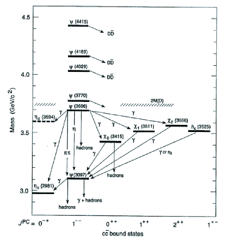
Figure 1:

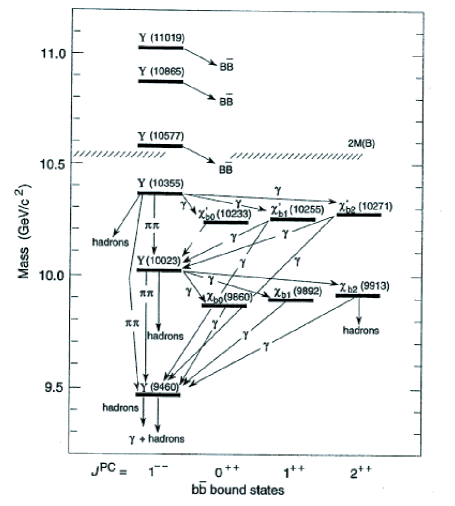
Figure 2:

What was found to be the ”good” condition to explain i) is that the central potential should be such that its Laplacian is positive [11].

We can state the following theorem:

Theorem  I
Let $E(n,\ell)$ be an energy level in a central potential, $n$ being the number of nodes of the radial wave function, $\ell$ the orbital angular moment. Then

$$E(n+1,\ell)^{>}_{<}~{}E(n,\ell+1)~{}~{}\rm{if}~{}~{}r^{2}\Delta~{}~{}V(r)^{>}_{<}~{}0~{}.$$ (1)

Now: why is this a good criteria, for the quark-antiquark potential. The answer is that this is a strong version of asymptotic freedom.

Call the force between a quark and an antiquark

$$-{dV\over dr}=F(r)=-{\alpha(r)\over r^{2}}$$ (2)

In the Coulomb case, $\alpha(r)$ is essentially constant and

$$\Delta V={1\over r^{2}}~{}~{}{d\over dr}~{}~{}r^{2}~{}{dV\over dr}=4\pi~{}~{}\delta^{3}(\overline{r})$$ (3)

i.e., $\Delta V=0$ outside the origin.

In QCD, asymptotic freedom can be expressed as

$${d\over dr}~{}~{}\alpha(r)>0~{},$$ (4)

where $\alpha(r)$ is the running coupling constant and hence $\Delta V(r)>0$.

Now let us come to ii). We know, since Newton (according to Markus Fierz), that there are two and only two kinds of forces for which all bound states have classical closed orbits: the Coulomb and harmonic oscillator forces.

Theorem I represents a comparison of the potential with the Coulomb potential. It might be interesting to compare the quark-antiquark potential with the harmonic oscillator potential, $V=r^{2}$. $V=a+br^{2}$ satisfies

$${d\over dr}~{}~{}{1\over r}~{}~{}{dV\over dr}=0$$

One can prove the following theorem [12].

Theorem II
If

$${d\over dr}~{}~{}{1\over r}~{}~{}{dV\over dr} {}^{>}_{<}~{}0~{}~{}~{}~{}~{}~{}~{}~{}~{}~{}~{}~{}~{}~{}$$ (5)

$$E(n+1,\ell) {}^{>}_{<}~{}E(n,\ell+2)$$ (6)

In the case of quarkonium, it has been shown by E. Seiler [13], from lattice QCD, that the quark-antiquark potential is concave and increasing. Hence

$${d\over dr}~{}~{}{1\over r}~{}~{}{dV\over dr}=-{1\over r^{2}}~{}~{}{dV\over dr}+{1\over r}~{}~{}{d^{2}V\over dr^{2}}<0$$

In this way, we understand that the mass of the $\psi^{"}$ $(n=0,\ell=2,)$ is higher than the mass of the $\psi^{\prime}~{}(n=1,\ell=0)$. We shall come back later on the question of why the $\ell=1$ states are above the average of the neighbouring two $\ell=0$ states.

Outside these two theorems on the level ordering there are others, where the criterium is the sign of $D_{\alpha}V(r)$ where

$$D_{\alpha}={d^{2}\over dr^{2}}+(5-3\alpha)~{}{1\over r}~{}~{}{d\over dr}+2(1-\alpha)~{}(2-\alpha)~{}{1\over r^{2}}$$ (7)

the previous cases correspond to

$$\alpha=1~{}~{}\rm{and}~{}~{}\alpha=2$$

These theorems are not optimal, but we have conjectured with a relatively strong basis that if

$$\left(r~{}{d^{2}\over dr^{2}}-(\alpha^{2}-3)~{}{d\over dr}\right)~{}V(r)\leq 0$$ (8)

with $\alpha>2$, then $E(n,\ell)<E(n-1,\ell+\alpha)$, for instance if we take

$$\begin{array}[]{ll}V(r)&=r^{4}\\ E(n,\ell)&<E(n-1,\ell+\sqrt{6})\end{array}$$

Indeed, for instance

$$\begin{array}[]{lll}E(1,0)&=11.6,~{}~{}E(0,\sqrt{6})&=12.6\\ E(1,5)&=35,7,~{}~{}E(0,5+\sqrt{6})&=36.3\end{array}$$

In another special case, $V(r)=r^{5}$ a rigorous but painful proof gives

$$E(n=0,\ell+\sqrt{7})>E(n=1,\ell)~{}.$$

Let us return now to Theorem I. So far it was applied to quarkonium, but there are other applications. The first one is muonic atoms. In muonic atoms, the Bohr radius is so small that the muon ”sees” the extension of the nucleus.

Since the nucleus, in the first approximation where it is supposed to be made of protons and neutrons, has a positive charge distribution, the potential exerted on the muon has a positive Laplacian and

$$E(n+1,\ell)>E(n,\ell+1)$$

This is indeed what was found in early calculations of muonic energy levels [14]. However, this was in fact independent of the details of the chosen charge distribution. This is seen experimentally. For instance, using the standard atomic spectroscopic notation, $N,\ell$, total angular momentum, with $N=n+\ell+1$, for $(\mu^{-}~{}~{}^{138}Ba)$ atoms [15]

$$\begin{array}[]{ll}2s_{1/2}-2p_{1/2}&=+405.41~{}~{}\rm{KeV}\\ 3p_{3/2}-3d_{3/2}&=~{}~{}~{}~{}~{}~{}8.69~{}~{}\rm{KeV}\end{array}$$

One might object that relativistic corrections cannot be neglected. However, it has been shown [16] (at least for perturbations around the Coulomb potential) that the inequalities survive for the Dirac equation as long as one compares levels with the same total angular momentum.

The other field where Theorem I is useful is atomic physics, in the approximation where the alcaline atoms can be treated as one outer electron plus a closed shell. The nucleus, seen from far away by the outer electron is now essentially pointlike and the effective potential is a Coulomb potential plus the result of a negative charge distribution. So it has a negative Laplacian. Take for instance Lithium. It has three electrons. Two of them form a closed shell. What will the outer electron be:

$$2s~{}~{}\rm{or}~{}2p~{}~{}?$$

It will be $2s$ because of the negativity of the Laplacian. In this way, Theorem I helps to understand many aspects of the Mendeleiff classification which, previously, were explained by not very convincing handwaving arguments. Figure 3, taken from [17] shows that these considerations hold also for excited states of the lithium atom.

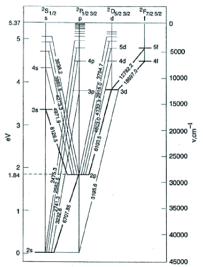
Figure 3:

One sees also that for large principal quantum numbers the Coulomb degeneracy tends to reappear. On Fig. 3, it is interesting to see that

$$3s<3p<3d$$

more precisely, one has, theoretically [18], and experimentally [19]:

$$3s_{1/2}~{}~{}~{}~{}~{}~{}<3p_{1/2}~{}~{}~{}~{}~{}~{}~{}<3p_{3/2}~{}~{}~{}~{}~{}~{}~{}<3d_{3/2}~{}~{}~{}~{}~{}~{}<3d_{5/2}$$ (9)

$$27206.066<30925.517<30925.613<31283.018<31283.053~{}~{}\rm{cm}^{-1}$$ (10)

These inequalities are valid for an outer electron satisfying the Dirac equation with a monotonous increasing potential such that $\Delta V<0$. The assumption of monotonicity is probably superfluous.

3 Spacing of Energy Levels

Since energy levels depend on two quantum numbers, $n$ and $\ell$, the problem is very broad and very difficult to explore completely. We shall restrict ourselves to two extreme cases:

• Compare the spacing of the energy levels for fixed $n$, and in fact we shall restrict ourselves to $n=0$, i.e., the purely angular excitations.

• Study the relative spacings of the energy levels for fixed $\ell$, specifically $\ell=0$.

While, for case a) there is a large amount of exact results, for case b) we have only imperfect indications. The results obtained in a), however, will allow us to answer question ii) in Section II.

In these problems a simple reference potential is the harmonic oscillator $V=r^{2}$. There all the fixed $n$, increasing $\ell$ spacings are equal and all the fixed $\ell$ increasing $n$ spacings are equal.

a) Spacing of purely angular excitations $n=0$, increasing $\ell$. There one gets easily

Theorem III [20]
If

$${d\over dr}~{}~{}{1\over r}~{}~{}{dV\over dr}<0$$ (11)

(12)

$${E(0,\ell+2)-E(0,\ell+1)\over E(0,\ell+1)-E(0,\ell)}<1$$ (13)

There exists also a differential form of this inequality.

If we combine this with Theorem II, which gives, under the same conditions

$$E(1,\ell)<E(0,\ell+2)$$

we get

$$E(0,\ell+1)>{1\over 2}~{}\left[E(0,\ell)+E(1,\ell)\right]$$

and the special case

$$E(0,1)>{1\over 2}\left[E(0,0)+E(1,0)\right]$$

which is precisely what is observed in the $c\overline{c}$ and $b\overline{b}$ spectra.

We would also like to have the analogue inequality for the second $\ell=1$ state, $E(1,1)$ but so far this is not the case.

A more subtle inequality for angular excitations is obtained if $\Delta V(r)^{>}_{<}~{}0$. Denote $E(0,\ell)$ as $E_{\ell}$, then

Theorem IV [21]
If

$${d\over dr}~{}r^{2}~{}{dV\over dr}~{}^{>}_{<}~{}0~{}~{},$$ (14)

(15)

$${E_{\ell+1}-E_{\ell}\over E_{\ell}-E_{\ell-1}}~{}{{}^{>}_{<}}~{}{2\ell+3\over 2\ell+1}~{}~{}\left({\ell\over\ell+2}\right)^{2}~{},$$ (16)

where the right-hand-side corresponds to the pure Coulomb case. Application to the $c\overline{c}$ system is rather frustrating. We get

$${E_{2}-E_{1}\over E_{1}-E_{0}}>{5\over 27}~{},$$

trivially satisfied by experiment.

Muonic atoms, on the other hand, are much more interesting. They also have $r^{2}\Delta V>0$ and the spacing between purely angular excitations is what is most easily observed by looking at cascading $\gamma$ rays by favoured electric dipole transitions. For small nuclear charge $Z$ or for large angular momenta the deviations for the Coulomb value are small while they are large for small $\ell$ and large $Z$.

After relativistic corrections, we get

Table 1

$Z$	${E_{3d}-E_{2p}\over E_{2p}-E_{1s}}$	${E_{4f}-E_{3d}\over E_{3d}-E_{2p}}$	${E_{5g}-E_{4f}\over E_{4f}-E_{3d}}$
$Z\rightarrow 0$	0.185	0.350	0.463
20	0.202	0.350	0.463
40	0.253	0.350	0.463
60	0.333	0.353	0.463
80	0.462	0.370	0.463

Conversely, for Alcaline atoms we have $\Delta V<0$. Here we just give the Lithium sequence, i.e., ions with three electrons and increasing charge. Here, it is just the reverse. When $Z$ gets large, the Coulomb limit is approched because the charge of the nucleus dominates on the electron cloud. For extremely large $Z$ (this is fictitious) the orbits are inside the cloud and do not see it.

Table 2

$Z$	${E_{4f}-E_{3d}\over E_{3d}-E_{2p}}$	${E_{5g}-E_{4f}\over E_{4f}-E_{3d}}$
3	0.326	0.462
6	0.329	0.462
9	0.334	0.462
12	0.338	0.462
15	0.339
$\infty$	0.350	0.463

Finally we give inequalities on the spacing between states with the same quantum numbers and different total angular momentum, i.e., the fine splitting. If, keeping $n=0$

$$\delta=E(\ell,J\equiv\ell+{1\over 2})-E(\ell,J^{\prime}=\ell-{1\over 2})$$ (17)

we have in the semi-relativistic approximation

$$\delta={2\ell+1\over 4m^{2}}\left<{dV\over dr}\right>$$ (18)

where the expectation value is to be taken using the Schrödinger wave function.

We have two theorems [21].

Theorem V

$$\delta(\ell)^{<}_{>}~{}\Delta(\ell)={2\over m\ell}~{}~{}{(\ell+2)^{4}\over(2\ell+3)^{2}}~{}~{}\left(E_{\ell+1}-E_{\ell}\right)^{2}$$ (19)

and

$${\delta(\ell+1)\over\delta(\ell)}^{>}_{<}~{}{\ell(\ell+1)^{3}\over(\ell+2)^{4}}~{}~{},~{}~{}~{}\rm{if}~{}~{}~{}r^{2}\Delta V(r)^{>}_{<}~{}0$$ (20)

for muonic atoms, i.e., $r^{2}\Delta V(r)>0$, we give only a sample of the results and forget the uncertainties to improve legibility

Table 3

$Z$	$\delta(1)$	$\Delta(1)$	$\delta(2)$	${\delta(2)\over\delta(1)}>0.098$
	in keV
26	4.2	4.4	0.47	0.112
33	11.10	11.45	2.00	0.18
41	23.15	29.10	2.68	0.116
50	45.7	60.60	5.65	0.123

Applications to Alcaline atoms, with $\Delta V<0$, are on the other hand rather disappointing. Let us remember that Eq. (12) is violated by the levels of the Sodium atom since the sign of the spacing of the well-known Sodium doublet (which produces by transition to the ground state the horrible yellow light) is the opposite. Exact treatment by the Dirac equation does not help. It is a typically many-body effect.

Concerning the lithium isoelectronic sequence, i.e., ions with three electrons, the situation is not as bad in the sense that $\delta(1)$ and $\delta(2)$ have the right sign. However, the inequality

$$\delta(1)>\Delta(1)~{}~{}\rm{and}~{}~{}\delta(2>\Delta(2)$$ (21)

are violated for Lithium itself. It is only for $Z\geq 6$ (Be II, etc.) that they are satisfied. This is seen in Table 4 (the units are cm^-1)

Table 4

$Z$	$\delta(1)$	$\Delta(1)$	$\delta(2)$	$\Delta(2)$	${\delta(2)\over\delta(1)}<0.098$
	in cm-1
3	0.337	0.422	0.037	0.036	0.1097
5	34.1	34.2	3.1	2.5	0.0909
6	107.1	106.6	10.5	9.278	0.098
9	975.8	962.7	90.0	87	0.092
12	3978	3938	470	362	0.0118
15	11310	11100	1000		0.088
24	90910	90000

We see also that $\delta(1)/\Delta(1)$ is always very close to unity. There are also inequalities of the same kind for hyperfine splittings but, for these, we refer to the original work [21].

We turn now to the problem of spacings between $\ell=0$ levels [22]. We present a number of incomplete results, which give strong indications, but completely rigorous proofs are lacking. Two things are certainly true:

• the $\ell=0$ levels of the harmonic oscillator potential are equally spaced, as everybody knows;

• the $\ell=0$ levels of the linear potential have a spacing decreasing with $n$.

We study now the neighbourhood of a), i.e., potentials close to the harmonic oscillator potential.

A preliminary remark is that the spacing between the $n=0$ levels will remain constant not only if we replace $r^{2}$ by $A~{}r^{2}+B$, but also if we add a $C/r^{2}$ term. Adding such a term is equivalent to changing the angular momentum by an (generally not integer) amount $\ell$ such that $C=\ell(\ell+1)$. Since the “Regge trajectories” of the harmonic oscillator are linear and parallel, the spacing between the energy levels will not change.

An interesting quantity to control the spacings is

$$Z(V,r)={d\over dr}~{}~{}r^{5}~{}~{}{d\over dr}~{}~{}{1\over r}~{}~{}{dV\over dr}$$ (22)

$Z$ vanishes for

$$V=\rm{const.},~{}~{}V=r^{2}~{},~{}~{}V={1\over r^{2}}~{}.$$ (23)

What we have proved, using a new kind of raising and lowering operators is that if

$$V=r^{2}+\lambda v~{}~{},$$ (24)

for $\lambda$ sufficiently small, the spacing between the energy levels increases with $n$ if $Z(V,r)>0$ $\forall r$ and the spacing between the energy levels decreases with $n$ if $Z(V,r)<0$ $\forall r$.

However, in the non-perturbative case, we do not know what happens. In fact we even have counter examples.

Take the “partially soluble” potential [23]

$$V=r^{6}-9r^{2}$$

the first five energy levels are given by

$$\left\{\begin{array}[]{ll}E_{0},E_{4}&=\mp\sqrt{480+96\sqrt{11}}\\ E_{1},E_{3}&=\mp\sqrt{480-96\sqrt{11}}\\ E_{2}&=0\end{array}\right.$$ (25)

Obviously, even though $Z(V,r)$ is positive, the levels show a symmetric pattern around $E_{2}=0$. However, there is no known counterexample in which $V$ is monotonous increasing.

We are tempted to make the conjecture that if $Z>0$ and if the potential is monotonous, the spacings increase, and if $Z<0$ and the potential is monotonous, the spacings decrease. “Experimental” tests with $V=r^{\alpha}$ indicate that the spacing increases with $n$ if $\alpha>2$ and decreases with $n$ if $\alpha<2$.

We study now the neighbourhood of b), the purely linear potential. Then the solutions of the Schrödinger equation are Airy functions. Then, the energy levels are given by $E_{n}=-r_{n-1}$, where $r_{n}$ is the $n^{th}$ zero of the Airy function. It is obvious that the spacing between $r_{n}$ and $r_{n+1}$ is smaller than the spacing between $r_{n-1}$ and $r_{n}$ because the potential is stronger.

We strongly believe that for all concave potentials, which correspond to the physical situation for quark-antiquark systems [13], the spacing between $\ell=0$ levels decreases with $n$. This is precisely what is indicated by the WKB approximation, in which we can regard $n$ as a continuous variable. The spacing will decrease if

$${d^{2}E\over d~{}n^{2}}<0~{},~{}~{}~{}{\rm{i.e.}}~{}~{}~{}{d^{2}n\over dE^{2}}>0~{}.$$

Indeed, in the WKB approximation

$${d^{2}n\over dE^{2}}= {1\over 2\pi}~{}~{}{1\over V^{\prime}(0)\sqrt{E-V(0)}}$$ (26)

$$-{1\over 2\pi}~{}~{}\int_{E-V>0}~{}~{}{V^{"}\over V^{\prime 2}\sqrt{E-V}}~{}~{}dr$$ (27)

which is positive if $V^{\prime}(0)>0$ and $V^{"}<0$.

The $b\overline{b}$ spectrum possesses this property, at least below the $B\overline{B}$ threshold [24]:

$$\begin{array}[]{ll}M_{\gamma^{\prime}}-M_{\gamma}&=560~{}\rm{MeV}\\ M_{\gamma^{"}}-M_{\gamma^{\prime}}&=332~{}\rm{MeV}\end{array}$$

4 The Wave Function at the Origin, the Kinetic Energy, etc.

Perhaps it is worth mentioning results on the wave function at the origin because one of the two papers which initially attracted the attention of Professor Zichichi is precisely on this subject [4].

The wave function at the origin appears in the so-called Van Royen-Weisskopf formula [25] (also proposed by Pietschmann and Thirring, M. Krammer and H. Krasemann) which controls the leptonic width of quarkonium:

$$\Gamma_{e^{+}e^{-}}=16\pi\propto e^{2}_{Q}~{}~{}{|\psi(0)|^{2}\over M^{2}}~{},$$ (28)

where $e_{Q}$ designate the charge of the quarks in units of $e$. $|\psi(0)|^{2}$ also controls the hadronic width, i.e., the decay into three gluons of quarkonium. The reduced wave function at the origin is given for the $\ell=0$ wave function by a formula attributed to Schwinger:

$$\left(u^{\prime}_{n}(0)\right)^{2}=2m\int^{\infty}_{0}~{}~{}{dV\over dr}~{}~{}u^{2}_{n}~{}~{}dr~{},$$ (29)

where

$$u={r\psi\over\sqrt{4\pi}}~{},$$

with

$$\int~{}~{}u^{2}_{r}~{}~{}dr=1$$

if $V$ is linear, ${dV\over dr}=$ const, and hence, because of the normalization of $u_{n}$, $|u^{\prime}_{n}(0)|^{2}$ and $|\psi_{n}(0)|^{2}$ are independent of $n$.

We proved the following theorem: if $V$ is concave, i.e., if $V^{"}<0$

$$|\psi_{1}(0)|^{2}<|\psi_{0}(0)|^{2}~{}~{},$$ (30)

if $V$ is convex, we get the reverse.

Indeed, even if you take into account the change of mass in the Weisskopf-Van Royen formula, experiment indicates that the leptonic widths of the $J/\psi$ and $\psi^{\prime}$ fit with a concave potential, which is what we expect from lattice QCD [13].

Can we go beyond that result? All we can say is that we have strong indications that the leptonic widths decrease with $n$ if $V$ is concave. For instance we can prove that $|\psi_{n}(0)|^{2}$ goes to zero for $n\rightarrow\infty$ if $V$ is concave.

Outside the wave function at the origin there are other quantities of interest on which we have a control, such as the mean kinetic energy, the root mean square radius, the electric dipole transition matrix elements, etc. For all these we send the reader to Ref. [9]. Let us just mention that this allows to set constraints on the “Schrödinger mass” of the quarks, if the potential is flavour independent, from the values of the $\ell=0$ and $\ell=1$ energy levels of the $c\overline{c}$ and $b\overline{b}$ systems:

$$m_{b}-m_{c}>3.29~{}\rm{GeV}~{},$$ (31)

while a naïve approach gives

$$m_{b}-m_{c}>{1\over 2}~{}\left(M_{b\overline{b}}-M_{c\overline{c}}\right)=3.18~{}\rm{GeV}$$ (32)

The mean kinetic energy of the system, $T$, that we call $T(m)$, where $m$ is the common quark mass in quarkonium, appears in the change in binding energy of a quark-antiquark system when the mass changes for a fixed potential (called flavour-independent for quarkonium), which is, from the Feynman-Hellman theorem

$${d\over dm}~{}~{}E(m)=-{T(m)\over m}$$ (33)

This proves already (25), from the positivity of $T$.

Now, with $M>m$

$$E(M)=E(m)-\int_{m}^{M}~{}~{}{T(\mu)\over\mu}~{}~{}d\mu$$

From the concavity with respect to any parameter entering linearly in the Hamiltonian, we get that $mT(m)$ is increasing with $m$. In fact, for a square well potential $mT(m)$ is constant.

However, if the potential is concave, which we believe from lattice QCD [13], we get a stronger result [26]:

$$m^{1/3}T(m){\bf{\nearrow}}$$ (34)

with $m$.

On the other hand, an inequality on $T(m)$ has been obtained [27]

$$T(m)>{3\over 4}~{}~{}\left[E(n=0,\ell=1,m)-E(n=0,\ell=0,m\right]~{},$$ (35)

which is saturatedby a harmonic oscillator potential.

From these considerations it is possible to get a lower limit to the mass difference between the $b$ quark mass and the $c$ quark mass, taking into account that the mass of a $Q\overline{Q}$ system is $2m_{Q}+E(m_{Q})$:

$$m_{b}-m_{c}>3.32~{}\rm{MeV}$$ (36)

Without (27), we would get the weaker result (24). This is only a sample of the many results obtained in this domain, for which we send the reader to Ref. [9].

5 A Fit of Heavy Quark Systems by a Potential Model

Now, we are leaving mathematical physics and turning to (dirty) phenomenology. After the discovery of the Upsilon and Upsilon prime systems by Lederman in 1977 [28], Quigg and Rosner made the remark that the spacing of the levels of the $c\overline{c}$ and $b\overline{b}$ systems is almost the same. If a potential model is acceptable, and if this potential is flavour independent, it is tempting to say that the potential could just be logarithmic, i.e., $C\ell n~{}r$. Then it is almost obvious that the spacings of all energy levels will be independent of the mass, because re-scaling $r$ to take into account the change of the mass will shift the potential by a constant. In 1981, I tried a small generalization of this by taking $V=A+Br^{\alpha}$, and adjusting $A,B$ and $\alpha$ to the known levels. I added too a Fermi-like hyperfine splitting to “explain” the $J/\psi-\eta_{c}$ mass difference. This seemed to be successful [29], [30], for mesons made of $b,c$ and even $s$ quarks and antiquarks. At the same time, Jean-Marc Richard, using the “rule” $V_{QQ}={1\over 2}~{}V_{Q\overline{Q}}$ reproduced beautifully the mass of the $\Omega^{-}$ baryon [31].

Then, my model was taken with disbelief by many physicists, including some friends, especially Russians, who could not understand how a naïve potential model could be justified. Most people preferred QCD sum rules, or lattice QCD, still in infancy.

However, I took the position that it was worth experimenting with this model even if it was difficult to justify. With time, many new particles and energy levels were discovered and happened to fit perfectly with this model. I remember a seminar by Lorenzo Foa, announcing the discovery of the $B_{s}$ meson by Aleph at LEP and saying that it was not necessary to give its mass because I had already predicted it. With, may be, one exception, this continues till now.

In fact, a first version including only $b$ and $c$ quarks was proposed [29]. However, seeing the incredible success of the fit, Murray Gell-Mann suggested that one should go further in the “absurd” (since $c$ quarks are not really non-relativistic) and include the strange quark. Let me give the numerical elements of the fit, made in 1981 [30], with the existing experimental information. The potential is

$$V=A+Br^{\alpha}$$

the fit gives

$$\begin{array}[]{ll}A&=-8.064\\ B&=~{}~{}~{}6.870~{},\end{array}$$

in units which are powers of GeV

$$\alpha=0.1$$

$$\begin{array}[]{ ll}m_{b}&=5.174\\ m_{c}&=1.8\\ m_{s}&=0.518\end{array}$$

(notice that this agrees with the lower limit (29) on $m_{b}-m_{c}$).

Futhermore, the large hyperfine splitting between $J/\psi$ and $\eta_{c}$ has to be taken into account by a phenomenological spin-spin interaction

$${C\over m_{1}m_{2}}~{}~{}(\sigma_{1}.\sigma_{2})~{}~{}\delta^{3}(\vec{r}_{1}-\vec{r}_{2})$$

$C$ is adjusted to the $J/\psi-\eta_{c}$ splitting.

Overall this is a seven parameter fit. We do not try to predict the fine splitting between the $\ell=1$ states and just predict the weighted average.

Table 5 gives the results. It contains 30 experimental numbers. It is an updated version of a table presented at the Montpellier 1997 conference [10]. The figures with stars are experimental results which were not known in 1981 (ten stars!). The fact that the $\eta^{\prime}_{c}$ is 15 MeV higher than predicted has been understood long ago because of the vicinity of the $D\bar{D}$ threshold (by J.-M. Richard).

Table 5

Masses and relative leptonic widths for $c\overline{c},b\overline{b},s\overline{s}$,

$c\overline{s},b\overline{s},b\overline{c}$, and of the $\Omega$ and $\Omega_{c}$ baryons.

Quark	States	Theory	Experiment	Theory	Experiment
System
$c\overline{c}$	$J/\psi$	3.095	3.097	1	1
	$\psi^{\prime}$	3.687	3.686	0.40	0.46 $\pm$ 0.06
	$\psi^{\prime\prime\prime}$	4.032	4.040	0.25	0.16 $\pm$ 0.02
	$\chi_{c}$ average	3.502	3.525
	and $h_{c}$
	$\psi^{"}$ average	3.787	3.770
	$\eta_{c}$	2.980	2.980
	$\eta^{\prime}_{c}$	3.641	3.656∗
$b\overline{b}$	$\Upsilon$	9.46	9.46	1	1
	$\Upsilon^{\prime}$	10.02	10.02	0.35	0.32 $\pm$ 0.05
	$\Upsilon^{"}$	10.36	10.35	0.27	0.24 $\pm$ 0.05
	$\Upsilon^{\prime\prime\prime}$	10.60	10.58	0.21	0.23 $\pm$ 0.06
	$\Upsilon^{iv}$	10.76	10.86 ∗
	$\chi^{b}$ average	9.86	9.90 ∗
	$\chi^{\prime}_{v}$	10.24	10.26 ∗
$s\overline{s}$	$\phi$	1.02	1.02
	$f_{1}$ average	1.42	1.44
	P state
	$\phi^{\prime}$	1.634	1.680
$c\overline{s}$	$D_{s}$	1.99	1.97
	$D^{*}_{s}$	2.11	2.11 ∗
	$D^{**}_{s}$ average	2.537	2.536 ∗
$b\overline{s}$	$B_{s}$	5.354	5.369 $\pm$ 0.005 ∗
	$B^{*}_{s}$	5.408	5.416 $\pm$ 0.004 ∗
$b\overline{c}$	$B_{c}$	6.25	6.4$\pm$ 0.39 $\pm$ 0.13 ∗
	$B^{*}_{c}$	6.32
$\Omega$		1.666	1.672
$\Omega_{c}$		2.708	2.697 $\pm$ 0.0025∗)
∗) These experimental numbers have been obtained after the initial fit in 1981.

We turn now to the baryon sector. Here we have been using the rule $V_{QQ}={1\over 2}~{}V_{Q\overline{Q}}$. Why this rule? A three quark system must be colour singlet. Hence in a three quark baryon, a quark pair must be a $\overline{3}$ colour state. So, if two quarks are close together, the third quark sees them as a $\overline{3}$ state, i.e., an antiquark. Hence the potential between the third quark and the quark pair is $V_{Q\overline{Q}}$. Dividing by two we get a potential ${1\over 2}~{}V_{Q\overline{Q}}$ between the third quark and each of the quarks of the pair.

This may seem doubtful but worth trying. Jean Marc Richard has done this for the $\Omega$ particle made of three strange quarks [31]. This gives $M_{\Omega}=1666$ MeV, to be compared with the experimental value 1672 MeV. Encouraged by this result we predict [32]

$$M_{\Omega_{c}}=2708~{}\rm{MeV},$$

which is now, experimentally [33] 2697.5 $\pm$ 2.5 MeV, only 10 MeV away.

Other predictions, still to be tested, are

$$\begin{array}[]{ll}M_{\Omega_{cc}}=3.737~{}\rm{MeV}\\ M_{\Omega_{ccc}}=4.787~{}\rm{MeV}\end{array}$$

The $ccc$ system, according to Bjorken [34], is one of the most interesting quark systems. It is stable with respect to strong interactions and has a lifetime of the order of $2\times 10^{-13}$ seconds. It might be difficult to produce, but, who knows, it might be seen at the LHC. After all, at LEP, many interesting particles such as $B_{s},B_{c}$ or $\Lambda_{b}$ were seen while their observation was not initially planned.

ACKNOWLEDGEMENTS

I have already mentioned, at the beginning, the crucial role of A. Zichichi, who, by asking me to lecture on quarkonium in Erice in 1977 induced me to investigate a whole field of research. This, I believe, turned out to be very fruitful. Among all those to whom I am grateful, I would like to single out, on the mathematical physics side, H. Grosse who co-signed with me the book ”Particle Physics and the Schrödinger Equation”, and also R. Bertlmann, A.K. Common and J. Stubbe, and on the phenomenological side, J.M. Richard. I am grateful to many other physicists (some are no longer with us): B. Baumgartner, M.A.B. Bég, J.S. Bell, R. Benguria, Ph. Blanchard. K. Chadan, T. Fulton, V. Glaser, A. Khare, J.D. Jackson, R. Jost, P. Landshoff, H. Lipkin, J.J. Loeffel, J. Pasupathy, C. Quigg, T. Regge, J. Rosner, A. De Rújula, A. Salam, P. Taxil.

Finally, I would like to thank my wife, Schu, for her strong moral support during the preparation of the 1977 lectures, and for her insistance to convince me to write a book with H. Grosse; I also thank M.N. Fontaine, who, though retired, typed this article because my brain is too rusty to learn Latex.

References

-
[1]
J.J. Aubert et al., Phys.Rev.Lett. 33 (1974) 1404;
J.E. Augustin et al., Phys.Rev.Lett. 33 (1974) 1406;
G.S. Abrams et al., Phys.Rev.Lett. 33 (1974) 1453. - [2] See, for instance: L. Maiani, in ”Elementary Processes at High Energy”, A. Zichichi ed., Academic Press, New York and London (1971) p. 600.
- [3] A. Martin, Phys.Lett. 67B (1977) 75.
- [4] A. Martin, Phys.Lett. 70B (1977) 192.
- [5] A. Martin, in ”The Whys of Subnuclear Physics”, A. Zichichi ed., Plenum Press, New York and London (1979), p. 395.
- [6] H. Grosse and A. Martin, Physics Reports 66 (1980) 341.
- [7] C. Quigg and J. Rosner, Physics Reports 56 (1979) 167.
- [8] A. Martin, in ”From Superstrings to the Real Super World”, International School of Subnuclear Physics, A. Zichichi ed., World Scientific, Singapore (1993) p. 482.
- [9] H. Grosse and A. Martin - Particle Physics and the Schrödinger Equation, Cambridge University Press (1977) ISBN 13978-0-521-39225-9.
- [10] A. Martin, Nucl.Phys. B (Proc.Suppl.) 54A (1977) 244.
-
[11]
B. Baumgartner, H. Grosse and A. Martin, Phys.Lett. B146 (1984) 363.
See also improved proofs:
M.S. Ashbaugh and R.D. Benguria, Phys.Lett. A131 (1988) 528, and
A. Martin, Phys.Lett. A147 (1990) 1. - [12] B. Baumgartner, H. Grosse and A. Martin, Nucl.Phys. B254 (1985) 528.
- [13] E. Seiler, Phys.Rev. D18 (1978) 133.
- [14] J.A. Wheeler, Rev.Mod.Phys. 21 (1949) 133.
- [15] R. Engfer et al., At. Data Nucl. Data Tables 14 (1991) 287.
- [16] H. Grosse, Phys.Lett. B197 (1987) 413.
- [17] E. Chpolsky, Physique Atomique, Moscow, Mir, French Translation (1978).
- [18] H. Grosse, A. Martin and J. Stubbe, Phys.Lett. B284 (1992) 347.
- [19] L.J. Radziemski et al., Phys.Rev. A52 (1995) 4462.
- [20] A.K. Common and A. Martin, Europhysics Lett. 4 (1987) 1349.
- [21] A. Martin and J. Stubbe, Europhysics Lett. 14 (1991) 287; Nucl.Phys. B367 (1991) 158.
- [22] A. Martin, J.M. Richard and P. Taxil, Nucl.Phys. B329 (1990) 327.
-
[23]
V. Singh, S.N. Biswas and K. Datta, Phys.Rev. D18 (1978) 1901. See also:
A.V. Turbiner Commun.Math.Phys. 118 (1988) 407. - [24] Review of Particle Physics, Phys.Lett. B592 (2004) 61,62.
-
[25]
R.P. Van Royen and V. Weisskopf, Nuovo Cimento 50A (1967) 617;
M. Krammer and H. Krasemann, Acta Physica Austriaca, Suppl. XXI (1979) 259. - [26] A.K. Common and A. Martin, J.Math.Phys. 30 (1989) 801.
- [27] R. Bertlmann and A. Martin, Nucl.Phys. B168 (1980) 111.
- [28] L. Lederman, Proceedings of the 1977 European Conference on Particle Physics, L. Jenik and I. Montvay eds., European Physical Society (1977), p. 303.
- [29] A. Martin, Phys.Lett. 93B (1980) 338.
- [30] A. Martin, Phys.Lett. 100B (1981) 511.
- [31] J.M. Richard, Phys.Lett. 100B (1981) 515.
- [32] A. Martin and J.M. Richard, Phys.Lett. B355 (1995) 345.
- [33] Ref. [24], p. 77.
- [34] B.J. Bjorken, in Proc. Int. Conf. on Hadron Spectroscopy, College Park 1985, ed. S. Oneda (A.I.P., New York 1985) p. 390.