Decoherence of many-spin systems in NMR:
From molecular characterization to an environmentally induced quantum dynamical phase transition
 

por
 

Gonzalo Agustín Álvarez

 

Presentado ante la Facultad de Matemática, Astronomía y Física
como parte de los requerimientos para acceder al grado de
Doctor en Física
de la
Universidad Nacional de Córdoba

Abstract

Decoherence of many-spin systems in NMR:

From molecular characterization to an environmentally induced quantum dynamical phase transition

The control of open quantum systems has a fundamental relevance for fields ranging from quantum information processing to nanotechnology. Typically, the system whose coherent dynamics one wants to manipulate, interacts with an environment that smoothly degrades its quantum dynamics. Thus, a precise understanding of the inner mechanisms of this process, called “decoherence”, is critical to develop strategies to control the quantum dynamics.

In this thesis we solved the generalized Liouville-von Neumann quantum master equation to obtain the dynamics of many-spin systems interacting with a spin bath. We also solve the spin dynamics within the Keldysh formalism. Both methods lead to identical solutions and together gave us the possibility to obtain numerous physical predictions that contrast well with Nuclear Magnetic Resonance experiments. We applied these tools for molecular characterizations, development of new numerical methodologies and the control of quantum dynamics in experimental implementations. But, more important, these results contributed to fundamental physical interpretations of how quantum dynamics behaves in open systems. In particular, we found a manifestation of an environmentally induced quantum dynamical phase transition.

Resumen

Decoherencia en sistemas de espines interactuantes en RMN:

De la caracterización molecular a una transición de fase en la dinámica cuántica inducida por el ambiente

El control de sistemas cuánticos abiertos tiene una relevancia fundamental en campos que van desde el procesamiento de la información cuántica hasta la nanotecnología. Típicamente, el sistema cuya dinámica coherente se desea manipular, interactúa con un ambiente que suavemente degrada su dinámica cuántica. Es así que el entendimiento preciso de los mecanismos internos de este proceso, llamado decoherencia, es crítico para el desarrollo de estrategias para el control de la dinámica cuántica.

En esta tesis usamos la ecuación maestra cuántica generalizada de Liouville-von Neumann para resolver la dinámica de sistemas de muchos espines interactuando con un baño de espines. También obtuvimos la dinámica de espines dentro del formalismo de Keldysh. Ambos métodos nos llevaron a idénticas soluciones y juntos nos dieron la posibilidad de realizar numerosas predicciones que concuerdan con las observaciones de experimentos de Resonancia Magnética Nuclear. Estos resultados son usados para la caracterización molecular, el desarrollo de nuevas metodologías numéricas y el control de la dinámica cuántica en implementaciones experimentales. Pero aún más importante es el surgimiento de interpretaciones físicas fundamentales de la dinámica cuántica de sistemas cuánticos abiertos, tales coma la manifestación de una transición de fase en la dinámica cuántica inducida por el ambiente.

Agradecimientos

Deseo expresar mi agradecimiento a muchas personas, que en diferentes “formas y medidas”, fueron contribuyendo a la finalización de este trabajo. Desde el comienzo del mismo, una de mis principales motivaciones fue formarme como físico; en este aspecto, desde mi punto de vista es esencial una fuerte complementación entre herramientas teóricas y experimentales para atacar los diversos problemas de la naturaleza. Es por ello, que estoy en especial muy agradecido con mi directora, Patricia Levstein, y mi co-director, Horacio Pastawski; quienes me brindaron su conocimiento y las formas de ver y hacer física. Patricia contribuyendo desde su punto de vista experimental y Horacio desde el teórico, ayudándome así a generar una formación teórica-experimental de cómo encarar la física. Le agradezco mucho a Patricia, además, por haberme ayudado en el pulido de la escritura de esta tesis, en el idioma inglés.

Estoy muy agradecido también con el jurado, que evaluó mi tesis, el Dr. Carlos Balseiro, Dr. Guido Raggio, Dr. Juan Pablo Paz y Dr. Pablo Serra, quienes leyeron mi trabajo y me aportaron comentarios muy interesantes.

También le agradezco a Jésus Raya, con quien fue muy grato e enriquecedor trabajar en mi estadía en Francia, quien me dio una visión complementaria a la de Patricia con respecto a las mediciones experimentales. A Jérôme Hirschinger por su hospitalidad y comentarios.

Le agradezco a Lucio Frydman, por su hospitalidad en mi pasantía en su laboratorio; pero mucho más importante por su contribución en mi formación y por haber compartido conmigo su forma de trabajo.

Agradezco también a mis compañeros de grupo, empezando por los más antiguos: Fernando Cucchietti, Luis Foa Torres, Ernesto Danieli y Elena Rufeil Fiori, quienes no sólo contribuyeron en mi formación compartiendo entre todos nuestro conocimiento, sino también por haber aportado calidez al ambiente de trabajo. Lo mismo agradezco a los más nuevos: Claudia Sánchez, Belén Franzoni, Hernán Calvo, Yamila Garro Linck, Axel Dente y Guillermo Ludueña.

A la gente del Lanais: Gustavo Monti, Mariano Zuriaga, Néstor Veglio, Karina Chattah, Rodolfo Acosta y a Fernando Zuriaga, quien numerosas veces me ayudó con mi rebelde computadora.

A la gente de administración, que con su mejor onda me ayudaron siempre.

A mis compañeros de oficina: Fernando Bonetto, Ana Majtey, Alejandro Ferrón, Santiago Pighin, Santiago Gómez, Marianela Carubelli, Josefina Perlo por haber colaborado para generar un espacio grato de trabajo.

Un muy especial agradecimiento a mi familia, por haberme bancado y apoyado en todo incondicionalmente y por su apoyo afectivo.

A todos mis amigos por su afecto y momentos de descuelgue. En especial a Lucas, Eduardo, Andrés y Sandra.

A quienes más tengo que agradecerles es: a Valeria, quien estuvo a mi lado gran parte de mi vida y de este trabajo, gracias por tu sostén; a Sol, que estuvo, en un momento muy crítico ayudándome a reenfocar mi esfuerzo y a Any que aguantó y sostuvo mi estado crítico durante la culminación de este trabajo.

Agradezco a CONICET por el apoyo económico, brindado a través de una beca doctoral para realizar este trabajo. A la instituciones, CONICET, ANPCyT, SECyT y Fundación Antorchas por el soporte económico para mi formación, tanto aquí como en el exterior.

Y a todos aquellos, que de una manera u otra me fueron apoyando y alentando para concretar este trabajo. A todos MUCHAS GRACIAS….

Chapter 1 Introduction

Quantum Mechanics was developed to describe the behavior of matter at very small scales, around the size of single atoms. Today, it is applied to almost every device that improves our quality of life, from medical to communication technology. Since it involves laws and concepts that challenge our intuition, it keeps having a revolutionary impact on the formulation of new philosophical and scientific concepts not totally solved today [Omn92, Sch04]. While the foundations of quantum mechanics were established in the early 20^th century, many fundamental aspects of the theory are still actively studied and this thesis intends to contribute to this knowledge.

1.1 What is quantum physics?

One of the main characteristics of quantum mechanics is that it involves many counterintuitive concepts such as the superposition states. They were illustrated by the Austrian physicist Erwin Schrödinger in 1935 by his famous Schrödinger’s cat thought experiment. In his words [Sch35]:

“One can even set up quite ridiculous cases. A cat is penned up in a steel chamber, along with the following device (which must be secured against direct interference by the cat): in a Geiger counter there is a tiny bit of radioactive substance, so small, that perhaps in the course of the hour one of the atoms decays, but also, with equal probability, perhaps none; if it happens, the counter tube discharges and through a relay releases a hammer which shatters a small flask of hydrocyanic acid. If one has left this entire system to itself for an hour, one would say that the cat still lives if meanwhile no atom has decayed. The psi-function of the entire system would express this by having in it the living and dead cat (pardon the expression) mixed or smeared out in equal parts.

It is typical of these cases that an indeterminacy originally restricted to the atomic domain becomes transformed into macroscopic indeterminacy, which can then be resolved by direct observation. That prevents us from so naively accepting as valid a ”blurred model” for representing reality. In itself it would not embody anything unclear or contradictory. There is a difference between a shaky or out-of-focus photograph and a snapshot of clouds and fog banks.”

Erwin Schrödinger

Figure 1.1: Cartoon description of the Schrödinger’s cat paradox. After an hour the cat is in a quantum superposition of coexisting alive and dead states. Only after opening the box we found the cat in a defined state. Figure extracted from http://en.wikipedia.org/wiki/Image:Katze.jpg.

Essentially, he states that if we put an alive cat in a box where, isolated from external interference, is in a situation where death has an appreciable probability, the cat’s state can only be described as a superposition of the possible state results (dead and alive), i.e. the two states at the same time. This situation is sometimes called quantum indeterminacy or the observer’s paradox: the observation or measurement itself affects an outcome, so that it can never be known what the outcome would have been, if it were not observed. The Schrödinger paper [Sch35] was part of a discussion of the Einstein, Podolsky and Rosen’s paradox [EPR35] that attempted to demonstrate the incompleteness of quantum mechanics. They said that quantum mechanics has a non-local effect on the physical reality. However, recent experiments refuted the principle of locality, invalidating the EPR’s paradox. The property that disturbed the authors was called entanglement (a superposition phenomenon) that could be described briefly as a “spooky action at a distance” as expressed in ref. [EPR35]. This was a very famous counterintuitive effect of quantum mechanics which leads very important physicists to mistrust of quantum theory. The entanglement property could be schematized by adding some condiments to the Schrödinger’s cat thought experiment. First of all, we may consider that the indeterminacy on the cat’s state is correlated with the state of the flask of hydrocyanic acid, i.e. if the cat is alive the flask is intact but if the cat is dead the flask is broken. We have here two elements or systems (the cat and the flask) in a superposition state $\left|\text{cat alive,flask intact}\right\rangle$ and $\left|\text{cat dead,flask broken}\right\rangle$ existing at the same time. Assuming that after an hour we can divide the box with a slide as shown in figure 1.1 and deactivate the trigger, we can separate as we want the two boxes. Then, if someone opens the cat’s box and sees the cat’s state, the state of the flask will be determined instantaneously without concerning the distance between them. This is only a cartoon description of what quantum entanglement is about, but for a further description we refer to Nielsen and Chuang (2000) [NC00] or chapter 6.

One of the most interesting effects of quantum superposition is the interference phenomenon consequence of the information indeterminacy of the quantum state (dead or alive). The famous double slit ideal experiment, as Richard Feynman said, contains everything you need to know about quantum mechanics. As shown in fig. 1.2 a), the experiment consists of a double slit where a particle (photon, electron, etc.) can pass and a screen where it is detected.

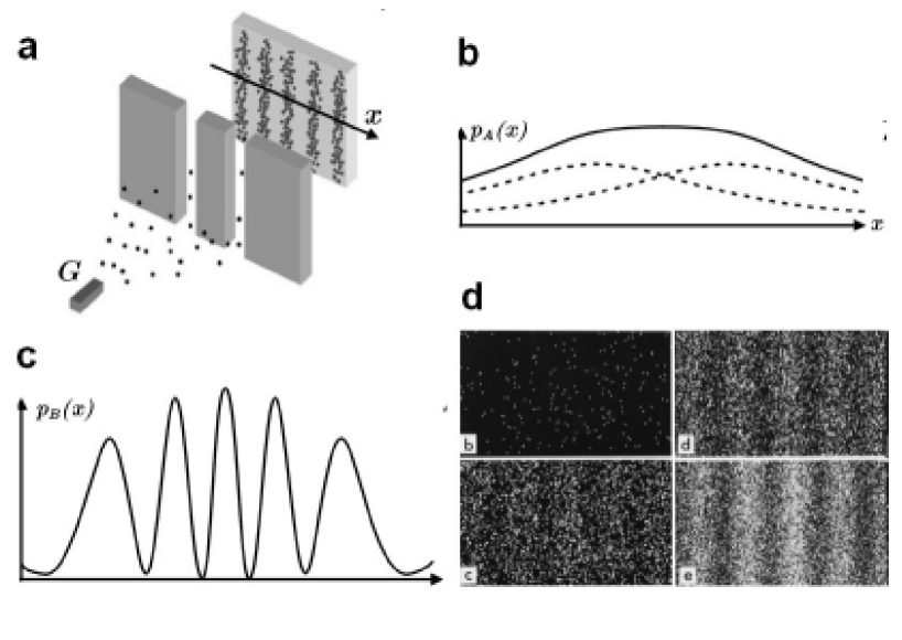
Figure 1.2: The double slit experiment. a) Schematic representation of the double slit device. b) The solid line is the classical probability prediction which is the sum of the individual one-slit probabilities. c) Interference pattern predicted by quantum probabilities accounting superposition. Panels b) and c) describe mathematical probabilities, in panel d) the physical reality is shown. The experiments were performed by A. Tonomura, et al. [TEM⁺89] where they showed that single electron events build up to form an interference pattern in the double-slit experiments. The number of electrons detected are 100, 3000, 20000 and 70000 respectively. Reprinted with permission from A. Tonomura, et al. Amer. J. Phys. Vol. 57, Issue 2, Page 117, 1989. Copyright 1989, American Association of Physics Teachers.

Behind it, there is a screen where we can register where the particle arrives. If only one of the slits is open, we have certainty that the particle only can pass through this slit. The probability to arrive to different places of the screen is shown in figure 1.2 b). There, we see that the most probable place for the particle arrival is obtained projecting the center of the slit to the register screen. Moving away from it, the probability decreases monotonically. The reciprocal situation occurs if only the other slit is open. However, if we leave the two slits open an interference pattern appears as in figure 1.2 c). Figures 1.2 b) and c) represent mathematical probabilities (mathematical reality) describing the physical reality shown in figure 1.2 d) [TEM⁺89].

Paul Kwiat, Harald Weintfurter and Anton Zeilinger making reference to quantum interference, in ref. [KWZ96], express:

“According to the rules of quantum mechanics, interference occurs whenever there is more than one possible way for a given outcome to happen, and the ways are not distinguishable by any means (this is a more general definition of interference than is often given in textbooks). In the double-slit experiment, light can reach the screen in two possible ways (from the upper or the lower slit), and no effort is made to determine which photons pass through which slit. If we somehow could determine which slit a photon passed through, there would be no interference, and the photon could end up anywhere on the screen. As a result, no fringe pattern would emerge. Simply put, without two indistinguishable paths, interference cannot occur.”

Paul Kwiat, Harald Weinfurter and Anton Zeilinger

Thus, the quantum mechanics is the physics of potentialities. When we have determinacy of some event, the classical physics appears. Nowadays, this appearance of the classical physics and state determinacy is considered a consequence of a phenomenon called decoherence [Zur03] which is the central topic of this thesis.

1.2 Decoherence: the degradation of quantum superpositions

The gedanken experiments introduced above must involve a perfect shielding from external influences allowing the existence of quantum superposition. Realistic quantum systems are never isolated, because they are immersed in an environment that continuously interacts with them. A typical environment consists of a system with many degrees of freedom that are hardly fully controlled or are not relevant for the observation. The system-environment (SE) interaction degrades the quantum superposition leading to the phenomenon called decoherence [Zur03, Sch04]. Actually, the measurement process to observe if the cat is dead or alive involves an interaction between the system (cat, acid, box, hammer, etc.) and the environment (observer, apparatus to observe, etc.). When the observation is performed, the cat is found either dead or alive, but not in the state dead and alive. The last one is a pure-state and the first one is a mixed-state. The decoherence process leads the system from a pure-state to a mixed-state. It is important to emphasize that, although quantum mechanics is open to many interpretations, decoherence by itself is neither an interpretation nor a modification of the theory. Thus, their existence can be taken as a well-confirmed fact. However, the implications that derive from decoherence could need some interpretations and this is one of the reasons why nowadays many researchers are devoted to its study [Zur03, Sch04].

Decoherence does not exist if we consider the entire system. It arises when we are interested in a particular part of the system leading to the consideration of a system plus an environment which is called an open system. Looking at the properties of the system, the environment modifies them leading to decoherence. It is at this point when the concept of the reduced density operator appears as a tool to mathematically describe the quantum world. A system is described by an entity called density operator, but the density operator of the Universe is impossible to obtain, thus one decides to reduce it to describe a relevant subsystem. The concept of the reduced density operator appeared together with quantum mechanics introduced by Lev Landau 1927 [Lan27] and further developed by John von Neumann 1932 [Neu32] and W.H. Furry 1936 [Fur36]. To illustrate the idea of how the reduced density matrix works, and why by observing at a subsystem we can not distinguish between a pure and a mixed-state, we consider a system with two entangled elements in a pure-state:

$$\left|\Psi\right\rangle=\frac{1}{\sqrt{2}}\left(\left|+\right\rangle_{1}\left|-\right\rangle_{2}-\left|-\right\rangle_{1}\left|+\right\rangle_{2}\right).$$ (1.1)

For an observable $\hat{O}$ that belongs only to the system $1$, i.e. $\hat{O}=\hat{O}_{1}\otimes\hat{1}_{2},$ the expectation value is given by

$$\left\langle\hat{O}\right\rangle_{\Psi}=\mathrm{Tr}\left\{\hat{\rho}\hat{O}\right\},$$ (1.2)

where the density operator of the pure-state is defined by

$$\hat{\rho}=\left|\Psi\right\rangle\left\langle\Psi\right|.$$ (1.3)

This statistical expectation value is defined as the sum of the values of the possible outcomes, multiplied by the probability of that outcome. The same statistics is applied to the reduced density operator that is obtained by tracing over the degrees of freedom of the system $2.$ Thus, we obtain

$$\left\langle\hat{O}\right\rangle_{\Psi}=\mathrm{Tr}\left\{\hat{\rho}\hat{O}\right\}=\mathrm{Tr}_{1}\left\{\hat{\sigma}_{1}\hat{O}_{1}\right\},$$ (1.4)

where the reduced density operator is

$$\hat{\sigma}_{1}=\mathrm{Tr}_{2}\left\{\left|\Psi\right\rangle\left\langle\Psi\right|\right\}=~{}_{2}\left\langle+|\Psi\right\rangle\left\langle\Psi|+\right\rangle_{2}+~{}_{2}\left\langle-|\Psi\right\rangle\left\langle\Psi|-\right\rangle_{2}.$$ (1.5)

Therefore, when the observer has access to a particular part of the system (system $1$), all the information obtainable through the subsystem is contained in the reduced density matrix (this assumes a statistical expectation value).

Noting that the states of the system $2$ are orthogonal, ${}_{2}\left\langle+|-\right\rangle_{2}=0,$ the reduced density matrix becomes diagonal

$$\hat{\sigma}_{1}=\mathrm{Tr}_{2}\left\{\left|\Psi\right\rangle\left\langle\Psi\right|\right\}=\frac{1}{2}\left(\left|+\right\rangle\left\langle+\right|\right)_{1}+\frac{1}{2}\left(\left|-\right\rangle\left\langle-\right|\right)_{1}.$$ (1.6)

This result corresponds to the density matrix of a mixed-state of the system $1$, i.e. in either one of the two states $\left|+\right\rangle_{1}$ and $\left|-\right\rangle_{1}$ with equal probabilities as opposed to the superposition state $\left|\Psi\right\rangle.$ A suitable interference experiment could confirm if it is a pure or a mixed-state, but if the observable belongs only to system $1$, the previous calculation demonstrates that it is impossible to distinguish between a pure or a mixed-state. We should not forget that this would not happen if the two elements, the system ($1$) and the environment ($2$) were not entangled. This demonstration could be extended to an arbitrary system of $N$ elements as discussed in ref. [Sch04]. While eq. (1.6) could be misinterpreted as it means that the state of the system is in both states at the same time, it is important to remark that the density matrix is a mathematical tool to calculate the probability distribution of a set of outcomes of a measurement of the physical reality but it does not represent a specific state of the system.

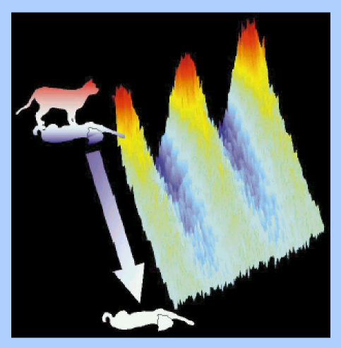
Figure 1.3: Schematic representation of decoherence showed in ref. [Sch00]. Decoherence slides the quantum world into the classical world. The oscillations from a quantum superposition of a single atom, being in two places at once, gradually die out to lead the atom to one definite place (either position). Reprinted by permission from Macmillan Publishers Ltd: Nature (W. P. Schleich, Nature 403, (2000) 256), copyright (2000).

Thus, the interaction of a quantum system with an environment destroys the quantum superposition leading the system to a statistical mixture of states. This process called decoherence has many implications in the foundations of quantum mechanics like the problem of quantum measurements, the quantum to classical transition and irreversibility [Zur03, Sch04]. But questions arise not only at a basic level. As a real quantum system can never be isolated, when the technology gives us the possibility to work with systems where quantum phenomena appear, the understanding of decoherence becomes relevant to exploit the potentialities of quantum superpositions .

In all the examples treated up to this point, the states constituting the quantum superposition have the same probability to exist. However, what happens when the probabilities are different? Moreover, what happens if the probabilities are time dependent? This leads to temporal interferences that appear in numerous experiments. For example, if we open each of the cat’s boxes in an ensemble, at one minute or after one hour the probability distribution of the cat’s state found is different. The same happens in the double slit experiment if there is an obstacle that blocks the slit oscillating between them. The interference pattern will be different depending on the time of observation. What happens now if we consider the environment effects? Including the SE interaction the quantum evolution is more complicated. There is no simple explanation for the appearance of decoherence because as we said previously one deals with an environment that has many degrees of freedom. More importantly, the decoherence affects the phases of the quantum superposition states, whose consequences are difficult to observe and understand. The first quantitative evaluation was given by Feynman and Veron (1963) [FV63] where they calculated dissipation through an environment of harmonic oscillators. Then, there were contributions from other people like K. Hepp and E.H. Lieb (1974) [HL73] and Wojciech Zurek (1981,1982) [Zur81, Zur82] who, while using less realistic models, suggest the universality of the effect and the relation with the measurement theory. However, the most complete work, in my opinion, was done by Caldeira and Legget (1983) [CL83c, CL83a, CL83b].

One of the first techniques, if not the first, in allowing the experimental control of the temporal evolution of quantum states was the nuclear magnetic resonance (NMR). In this thesis, we consider NMR experiments in connection with the physical reality of the theoretical interpretations.

1.3 NMR: The workhorse of quantum mechanics

The origins of Nuclear Magnetic Resonance dates from 1930 when Isidor Isaac Rabi discovered a technique for measuring the magnetic characteristics of atomic nuclei. Rabi’s technique was based on the resonance principle first described by Irish physicist Joseph Larmor, and it enabled more precise measurements of nuclear magnetic moments than had ever been previously possible. Rabi’s method was later independently improved upon by physicists Edward Purcell and Felix Bloch in 1945 [BHP46a, Blo46, BHP46b, PTP46, PPB46]. Later on, the technique was improved by the advent of fast computers and the development of pulse techniques that, through the Fourier transform, used the temporal evolution of the signal to notably optimize the acquisition time. The first experimental observations of the temporal evolution of a two-state system were done by H.C. Torrey (1949) [Tor49] and Erwin Hahn (1950) [Hah50a] where essentially a $1/2$-spin system (two-state system) is under the presence of a static field $H_{0},$ which splits the energy levels of the states $\left|+\right\rangle$ and $\left|-\right\rangle$ of each spin [see fig. 1.4 a)].

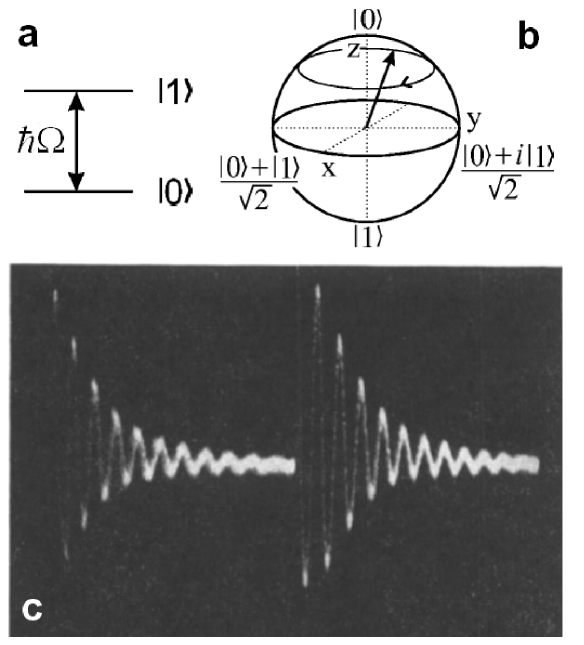
Figure 1.4: Oscillation between two states and the free induction decay. a) Energy splitting, $\hbar\Omega$, of the states of a spin $1/2.$b) Scheme of the spin precession around the static field. c) Experimental free induction decay obtained by E. Hahn (1950) [Hah50a]. Reprinted figure with permission from E. L. Hahn, Phys. Rev. 77, 297 (1950). Copyright (1950) by the American Physical Society.

Then, through a transversal field with a radio-frequency (RF) pulse, one can build a superposition state $a\left|+\right\rangle+b\left|-\right\rangle$ whose dynamics can be interpreted as a classical precession around the static field direction with the Larmor frequency $\Omega$ [see fig. 1.4 b)]. Fig. 1.4 c) shows the original experimental data taken by Hahn [Hah50a], where one can observe, after detection, a manifestation of the oscillation between the two states in an ensemble of spins. The attenuation of the oscillations is a consequence of the interaction with the environment, the other degrees of freedom that are not controlled and not observed. The simplest description of the experiment is to consider one spin and the other spins representing a spin-bath (the environment) whose interaction with the system (the selected spin) leads to decohere at a characteristic time $T_{2}$ called the spin-spin relaxation time.

From its fundamental beginnings, the NMR technique turned out soon into a precise spectroscopy of complex molecules which triggered impressive instrumental developments. However, nuclear spins and NMR keep providing wonderful models and continued inspiration for the advance of coherent control over other coupled quantum systems. It has gained the role of the workhorse of quantum dynamics. NMR was involved in the beginning of the experimental quantum information processing (QIP) applications, although nowadays, it is not considered feasible because its difficult scalability [QCR04]. However, in Vandersypen and Chuang words [VC04], NMR

“being one of the oldest areas of quantum physics[, give us the possibility to play with quantum mechanics because it] made possible the application of a menagerie of new and previously existing control techniques, such as simultaneous and shaped pulses, composite pulses, refocusing schemes, and effective Hamiltonians. These techniques allow control and compensation for a variety of imperfections and experimental artifacts invariably present in real physical systems, such as pulse imperfections, Bloch-Siegert shifts, undesired multiple-spin couplings, field inhomogeneities, and imprecise system Hamiltonians.

The problem of control of multiple coupled quantum systems is a signature topic for NMR and can be summarized as follows: given a system with Hamiltonian $\widehat{\mathcal{H}}=\widehat{\mathcal{H}}_{\mathrm{sys}}+\widehat{\mathcal{H}}_{\mathrm{control}}$, where $\widehat{\mathcal{H}}_{\mathrm{sys}}$ is the Hamiltonian in the absence of any active control, and $\widehat{\mathcal{H}}_{\mathrm{control}}$ describes terms that are under external control, how can a desired unitary transformation $\widehat{U}$ be implemented, in the presence of imperfections, and using minimal resources? Similar to other scenarios in which quantum control is a welldeveloped idea, such as in laser excitation of chemical reactions [Walmsley and Rabitz, 2003], $\widehat{\mathcal{H}}_{\mathrm{control}}$ arises from precisely timed sequences of multiple pulses of electromagnetic radiation, applied phase-coherently, with different pulse widths, frequencies, phases, and amplitudes. However, importantly, in contrast to other areas of quantum control, in NMR $\widehat{\mathcal{H}}_{\mathrm{sys}}$ is composed from multiple distinct physical pieces, i.e., the individual nuclear spins, providing the tensor product Hilbert space structure vital to quantum computation. Furthermore, the NMR systems employed in quantum computation are better approximated as being closed, as opposed to open quantum systems.”

Vandersypen and Chuang.

Thus NMR inspired other techniques in the methodology of quantum control [PJT⁺05]. In fact, the first realization of a SWAP operation in solids, an essential building block for QIP, could be traced back to a pioneer NMR experiment by Müller, Kumar, Baumann and Ernst (1974) [MKBE74]. While they did not intended it as a QIP operation, they described theoretically and experimentally the swapping dynamics (cross polarization) of two strong interacting spin systems and had to deal with the coupling to a spin-bath. Until that moment, all the experiments considering two interacting spins were treated through hydrodynamical equations [For90] using the spin-temperature hypothesis that leads to a simple exponential dynamics. Müller, et al. (MKBE) showed that, in a case where the coupling between two spins is stronger than with the rest, one has to consider quantum coherences in the quantum calculations. They modeled the experiment treating quantum mechanically the two-spin system and considering the coupling with the spin-bath in a phenomenological way as a relaxation process. The original figure published in the paper is shown in fig. 1.5,

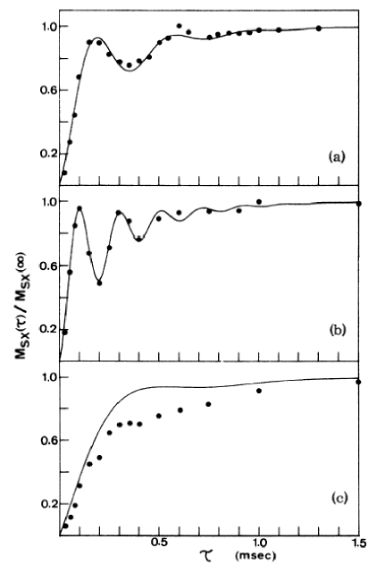
Figure 1.5: Transient oscillations in a cross-polarization experiment by Müller, Kumar, Baumann and Ernst (1974) [MKBE74]. The two-spin dynamics coupled to a spin-bath is shown for three different internal couplings. Reprinted figure with permission from L. Müller, A. Kumar, T. Baumann and R. R. Ernst, Phys. Rev. Lett. 32, 1402 (1974). Copyright (1974) by the American Physical Society.

where typical cross-polarization (swapping) dynamics for three different internal interactions (coupling between the two-spins) in ferrocene are displayed. One can clearly observe the frequency change of the quantum oscillation. More recent experiments, spanning the internal interaction strength were done by P. R. Levstein, G. Usaj and H. M. Pastawski [LUP98]. By using the model of MKBE [MKBE74], they obtained the oscillation frequency and the relaxation for different interaction strengths. These results are shown in fig. 1.6

Figure 1.6: Fitting parameters of a two-spin cross-polarization experiment performed by P. R. Levstein, G. Usaj and H. M. Pastawski (1998) [LUP98]. Striking changes in the relaxation and in the oscillation frequency behaviour are observed. These effect are described in chapter 4. Reprinted with permission from P. Levstein, G. Usaj and H. M. Pastawski, J. Chem. Phys. Vol. 108, Issue 7, Page 2718, 1998. Copyright 1998, American Institute of Physics.

where one can observe striking changes in the relaxation time and frequency as a function of the control parameter. Since this discontinuous change is not predicted by the standard model of MKBE, it remained unexplained. The description and interpretation of this striking behavior are among the main results of this thesis.

Thus, in view of possible applications to fields like quantum information processing [Kan98, BD00], the experimental manifestation of these dynamical interference phenomena in qubit clusters of intermediate size has a great interest. However, experimental realizations and control of a pure-state dynamics is still one of the challenges in nowadays physics [QCR04]. Therefore, one generally has to deal with an ensemble evolution, which is the case of the states involved in NMR, i.e. the dynamics of an initial mixed-state. One can generate mixed-states that are called pseudo-pure because they are constituted by a pure-state plus a mixed-state density operator. Numerous spin dynamics NMR experiments have shown surprising quantum phenomena [PLU95, MBSH⁺97, RSB⁺05]. The difficulty to produce pure-states in a high temperature sample leads to the development of the ensemble quantum computation [VSC04, SSB05]. However, as we mention previously if the system is too complex, it is hard to mathematically describe its temporal evolution. This is a consequence of the exponential growing of the Hilbert space dimension as a function of the number of elements in the system. In order to overcome this limitation, we take profit of the quantum parallelism [SKL02] and the fragility of the quantum superpositions to develop a method that describes ensemble dynamics.

As the dimension of the system increases, the sensitivity of the quantum superposition might lead to the inference that quantum phenomena will not manifest at macroscopic scales [MKT⁺00, Sch00]. In contrast, an experimental demonstration of macroscopic quantum states done by Y. Nakamura, et al. [NPT99, Ave99] shows the opposite. Indeed, there is no doubt about the high sensitivity of the quantum superposition states in large systems which paves the way for an effective decoherence when there are interactions with the environment. As any environment usually has many degrees of freedom, it is very difficult to reverse the SE interaction constituting the dominant source of irreversibility in nature [Zur03, Sch04]. Numerous works are related to this topic, but we should begin discussing the pioneer work that made a temporal reversion of a quantum dynamics: the Hahn’s echo experiment. It is based on the reversion of the dephasing among rotating spins due to inhomogenities of the static field [Hah50b]. He observed an echo in the NMR polarization signal (see fig. 1.7)

Figure 1.7: First experimental time reversion in NMR: The Hahn’s echo [Hah50b]. Reprinted figure with permission from E. L. Hahn, Phys. Rev. 80, 580 (1950). Copyright (1950) by the American Physical Society.

manifesting the deterministic nature of quantum mechanics, but with an attenuation rate proportional to the spin-spin coupling. The forward dynamics is a consequence of the interaction of the spins with the static field and the spin-spin interactions, but only the interactions with the static field are reverted. Thus, the dipolar interaction remains working. Within the NMR field, there were many experiments using the deterministic nature of quantum mechanics to take out some interactions that disturb the relevant system evolution. But, the first work that emphasizes the deterministic nature of quantum mechanics, invalidating the spin temperature hypothesis (thermodynamical approaches), was done by W. -K. Rhim and A. Pines and J. S. Waugh [RPW70]. They called a “Loschmidt daemon” to the process of reversion of the dipolar interaction in the “magic echoes” experiment. There, they observed an echo signal after undoing (reversion control) the evolution under spin-spin interactions that remain untouched in the Hahn’s echo experiment. The previous experiments evolve from multi-spin initial excitations. The local initial excitation version of the “magic echoes” was done by S. Zhang, B. H. Meier and R. R. Ernst (1992) [ZME92b]. They called this experiment as “the polarization echo” where they used a very ingenious idea to observe a local magnetization [ZME92b, ZME92a]. They used a rare nucleus, ¹³C, bonded to a ¹H nucleus (abundant) as a local probe to create and observe the local polarization. However, we have to remark that while one increases the quantum control on the Hamiltonians, a minimal decay of the echoes can not be avoided. Experiments performed in Córdoba suggest that the quantum states are so sensitive to perturbations that even a very small uncontrolled perturbation generates an intrinsic irreversibility characterized by the own system dynamics [LUP98, UPL98, PLU⁺00]. By considering an analogy with the behavior of a simpler one body chaotic system, this was interpreted [JP01, JSB01, CPJ04] as the onset of a Lyapunov phase, where $1/\tau_{\phi}=\min\left[1/\tau_{\mathrm{SE}},\lambda\right]$ is controlled by the system’s own complexity $\lambda$. However, a theoretical answer for many-body systems that do not have a classical analogue characterized by Lyapunov exponent remains open. This is also a topic that enters in this thesis’ motivation: the improvement of our comprehension and control of decoherence processes and irreversibility. The complexity of many-body systems leads us to study the forward dynamics of open systems to characterize the decoherence process before studying the time reversal.

1.4 Our contribution

In this thesis, we solve the dynamics of many-spin systems interacting with a spin-bath through the generalized Liouville-von Neumann quantum master equation beyond the standard approximation. Further consideration of the explicit dynamics of the bath helps us to solve the spin dynamics within the Keldysh formalism, where the interaction with the bath is taken into account in a precisely perturbative method based on Feynman diagrams. Both methods lead to identical solutions and together gave us the possibility to obtain numerous physical interpretations contrasting with NMR experiments. We used these solutions in conjunction with experimental data to design new protocols for molecular characterization, develop new numerical methodologies and control the quantum dynamics for experimental implementations. But, most important, these developments contributed to improve the fundamental physical interpretations of the dynamics in a quantum open system under the presence of an environment. In particular, we show a manifestation of an environmentally induced quantum dynamical phase transition.

1.4.1 Organization of this thesis

In Chapter 2 we use the standard formalism of density matrix to solve the spin dynamics using the generalized Liouville-von Neumann quantum master equation. In the first part of the chapter, the spin dynamics of a two-spin system coupled with a fast fluctuating spin-bath is solved. This system describes the cross-polarization experiment of MKBE [MKBE74]. We start using the standard approximations and then we extend the solution without these restrictions. We compare the solutions and remark the main differences. We analyze the spin dynamics for different anisotropies of the SE interactions given by the different contributions of the Ising and the XY interaction. We show how the rates of decoherence and dissipation change depending on the anisotropy ratio between the Ising and XY coupling. In the second part of the chapter, we extend the solution to a three-spin system coupled with a spin-bath. The solutions obtained are applied to experimental data to get more detailed information for molecular characterization. In particular, we use the three-spin solution to characterize the liquid crystal $8$CB and incorporating some memory effects, we conclude that the spin-bath has a slow dynamics.

In Chapter 3 we solve the spin dynamics within the Keldysh formalism [Kel64]. The Keldysh formalism is well established in the electron transport description. Through the Jordan-Wigner transformation [JW28], we map the two-spin system of chapter $2$ into a fermion system. We find how to describe the SE interaction within the wide band approximation (fast fluctuation inside the bath) and we obtain a solution for the spin dynamics that improves the standard solution of the generalized Liouville-von Neumann quantum master equation. Here, we use a microscopic model to obtain the spin dynamics that avoids using a phenomenological description of the SE interaction. However, we obtain the same solution going beyond the standard approximation within the density matrix formalism. Then, we solve the spin dynamics of a linear chain including all the degrees of freedom of the environment in the calculations and we show how the memory effects induce a time dependence in the oscillation frequency as is observed experimentally. We develop a stroboscopic model to describe decoherence which is optimized for numerical applications. This model converges to the continuous expression.

In Chapter 4 based on the solutions obtained in previous chapters we describe a manifestation of an environmentally induced quantum dynamical phase transition. We show the experimental evidence and interpret the phenomenon in detail. In particular, we show how the anisotropy of the SE interaction has an important role in the critical point of the phase transition. An extension of this phenomenon to a three-spin system shows how to vary the control parameter to “isolate” two of them from the environment.

In Chapter 5, inspired in the stroboscopic model developed in chapter 3, we propose a new NMR pulse sequence to improve the transfer of polarization through a specific pathway in a system of many interacting spins. The sequence effectively prunes branches of spins, where no polarization is required, during the polarization transfer procedure. Simulations of the spin dynamics in the ¹³C backbone of leucine are performed. Possible applications and potential fundamental contributions to engineered decoherence are discussed.

In Chapter 6 we develop a novel numerical method to obtain the spin dynamics of an ensemble. It overcomes the limitations of standard numerical calculations for large number of spins because it does not involve ensemble averaging. We exploit quantum parallelism [SKL02] and the fragility of a randomly correlated entangled state to reproduce an ensemble dynamics.

In the final part of each chapter a brief summary of the main original contributions including references to publications is included.

In Chapter 7 we summarize the whole work emphasizing the main conclusions and perspectives.

Chapter 2 Many-spin quantum dynamics within the density matrix formalism

The exact quantum dynamics of small quantum systems has regained interest during the last years [ALW92], due to the technological advances that give us the opportunity to observe quantum phenomena. Spin systems are good candidates in this respect and provide beautiful playgrounds for fundamental studies. Besides, several challenging applications require a very fine knowledge of the spin interactions, such as molecular characterization, spin control in nanodevices [SKE⁺01, KLG02] and quantum computation [GC97, CPH98, BD00]. In the introduction became evident the limitations of simple thermodynamical arguments [For90] based on the spin temperature hypothesis. The experiment of MKBE [MKBE74] showed the need to consider the system quantum mechanically keeping the quantum coherences to describe the transient oscillations. However, the first work that showed the weakness of the “spin temperature” hypothesis was done in 1970 [RPW70]. In it, a time reversal of the spin-spin interactions was performed. It was followed by numerous nuclear magnetic resonance (NMR) experiments that have demonstrated the time reversibility of the dipolar (many-spin) evolution [ZME92b, EMTP98a, EMTP98b, LUP98, UPL98] leading to revise the concept of “spin diffusion” [PLU95, PUL96, MBSH⁺97, Wau98]. More importantly, by selecting appropriate systems and pulse sequences, one can investigate the sources of quantum decoherence [Zur03, Sch04], ergodicity [PLU95, PUL96, Wau98], and quasi-equilibrium [SHE98].

From a practical point of view, spin dynamics observed by NMR has proved very powerful in order to characterize molecular structures and dynamics [SRS96]. Experimental observations together with simple analytical solutions for few-spin dynamics can provide detailed information on the intra and intermolecular interactions [MKBE74, LUP98, UPL98]. This is particularly important for the characterization of complex fluids in their native state, where one uses cross-polarization (CP) dynamics [HH62, Sli92] to evaluate order parameters [PR96]. However, the reliability of these and other structural and dynamical parameters depends on the accuracy of the spin dynamics description to which the experimental data are fitted.

In this chapter, we use the standard formalism of density matrix to solve the spin dynamics using the generalized Liouville-von Neumann quantum master equation [Abr61, EBW91]. In the first part of the chapter, we solve the spin dynamics of a two-spin system coupled to a fast fluctuating spin-bath. This system describes the cross-polarization experiment of MKBE [MKBE74]. As a first step, we use the standard approximations and then we extend the solution releasing these restrictions. We compare the solutions and remark the main differences. We analyze the spin dynamics for different SE interactions consisting of different Ising and XY contributions. We show how the decoherence and dissipation rates change depending on the anisotropy ratio between the Ising and XY couplings. In the second part of the chapter, we extend the solutions to a three-spin system coupled to a spin-bath. The solutions are applied to get more detailed information from our NMR experimental data. This leads to new methodologies for molecular characterization. In particular, we use the three-spin solution to characterize the liquid crystal $8$CB. The slow dynamics of the smectic phase, experimentally observed, lead us to include some spin-bath memory effects.

2.1 Quantum dynamics of a two-spin system

For didactical reasons, we start solving the spin dynamics of an isolated two-spin system. Then, we will include the interactions with the spin-bath.

2.1.1 Quantum evolution of an isolated two-spin system

We solve the evolution of an isolated two-spin system during cross-polarization (CP).

In this procedure, two different species of spins, $S$-$I,$ which here will correspond to a ¹³C-¹H system are coupled in such a way that they  “believe” that they are of the same species [Abr61, Sli92, EBW91]. In that situation, the most efficient polarization transfer can occur. The system Hamiltonian, in presence of a static field $H_{0}$ and the radio frequency fields of amplitudes $H_{1,S}$ and $H_{1,I}$ with frequencies $\omega_{\mathrm{rf},S}$ and $\omega_{\mathrm{rf},I}$ respectively, is given by [Abr61, Sli92]

$$\widehat{\mathcal{H}}_{\mathrm{S}}\mathcal{=-}\hbar\Omega_{0,S}\hat{S}^{z}-\hbar\Omega_{0,I}\hat{I}^{z}\\ -\hbar\Omega_{1,S}\left\{\hat{S}^{x}\cos\left(\omega_{\mathrm{rf},S}~{}t\right)+\hat{S}^{y}\mathop{\rm sen}\nolimits\left(\omega_{\mathrm{rf},S}~{}t\right)\right\}-\hbar\Omega_{1,I}\left\{\hat{I}^{x}\cos\left(\omega_{\mathrm{rf},S}~{}t\right)+\hat{I}^{y}\mathop{\rm sen}\nolimits\left(\omega_{\mathrm{rf},S}~{}t\right)\right\}\\ +2b\hat{I}^{z}\hat{S}^{z},$$ (2.1)

where

$$\Omega_{0,i}=\gamma_{i}H_{0,i},i=S,I$$ (2.2)

are the precession Larmor frequencies in the static field and

$$\Omega_{1,i}=\gamma_{i}H_{1,i},i=S,I$$ (2.3)

are the Zeeman (nutation) frequencies of the RF fields. The last term is the truncated dipolar interaction assuming that

$$\left|\hbar\Omega_{0,I}-\hbar\Omega_{0,S}\right|\gg\left|b\right|.$$ (2.4)

The amplitude of the interaction is [Sli92]

$$b=-\frac{1}{2}\left(\frac{\mu_{0}\gamma_{I}\gamma_{S}\hbar^{2}}{4\pi r^{3}}\right)\left(3\cos^{2}\theta-1\right),$$ (2.5)

where $r$ is the internuclear distance and $\theta$ the angle between the static field and the internuclear vector. In the double rotating frame [Sli92], at the frequencies of the RF fields, the system Hamiltonian becomes

$$\widehat{\mathcal{H}}_{\mathrm{S}}\mathcal{=}\hbar\Delta\Omega_{S}\hat{S}^{z}+\hbar\Delta\Omega_{I}\hat{I}^{z}-\hbar\Omega_{1,S}\hat{S}^{x}-\hbar\Omega_{1,I}\hat{I}^{x}+2b\hat{S}^{z}\hat{I}^{z}$$ (2.6)

where

$$\Delta\Omega_{i}=\Omega_{0,i}-\omega_{\mathrm{rf},i}$$ (2.7)

are the respective off-resonance shifts with $i=I,S$ . We assume the conditions

$$\Delta\Omega_{I}=\Delta\Omega_{S}=0$$ (2.8)

and

$$\hbar\left|\Omega_{1,S}+\Omega_{1,I}\right|\gg\left|b\right|$$ (2.9)

which are obtained when the RF fields are applied on-resonance and when the RF power is much bigger than the dipolar interaction. Thus, the doubly truncated Hamiltonian becomes

$$\widehat{\mathcal{H}}_{\mathrm{S}} \mathcal{=}\tfrac{1}{2}\left(\Sigma-\Delta\right)\hat{S}^{x}+\tfrac{1}{2}\left(\Sigma+\Delta\right)\hat{I}^{x}+b\left(\hat{S}^{z}\hat{I}^{z}+\hat{S}^{y}\hat{I}^{y}\right)$$ (2.10)

$$=\tfrac{1}{2}\Sigma\left(\hat{S}^{x}+\hat{I}^{x}\right)+\tfrac{1}{2}\Delta\left(\hat{I}^{x}-\hat{S}^{x}\right)+b\left(\hat{S}^{z}\hat{I}^{z}+\hat{S}^{y}\hat{I}^{y}\right),$$ (2.11)

where the non-secular elements of the dipolar interaction with respect to the $\Sigma\left(S^{x}+I^{x}\right)$ term have been neglected. Here, $\Sigma$ and $\Delta$ are defined by

$$\Sigma=-\hbar\left(\Omega_{1,S}+\Omega_{1,I}\right)~{}~{}~{}~{}~{}~{}~{}\text{and}~{}~{}~{}~{}~{}~{}~{}\Delta=\hbar\left(\Omega_{1,S}-\Omega_{1,I}\right).$$ (2.12)

Within the Hartmann-Hahn condition [HH62, Sli92], $\Delta=0,$ the two spins act as they belong to the same species improving the polarization transfer between them. To obtain the quantum evolution, we solve the Liouville-von Neumann equation [Abr61, EBW91]

$$\frac{\mathrm{d}}{\mathrm{d}t}\hat{\rho}(t)=-\frac{\mathrm{i}}{\hbar}\left[\widehat{\mathcal{H}}_{\mathrm{S}},\hat{\rho}(t)\right],$$ (2.13)

where $\hat{\rho}$ is the density matrix operator of the two-spin system. Its solution is given by

$$\hat{\rho}(t)=\hat{U}(t)\hat{\rho}(0)\hat{U}^{-1}(t),$$ (2.14)

with

$$\hat{U}(t)=\exp\left(-\frac{\mathrm{i}}{{}^{\hbar}}\widehat{\mathcal{H}}_{\mathrm{S}}t\right)$$ (2.15)

the evolution operator and $\hat{\rho}\left(0\right)$ the initial condition. For the last, we consider the ¹H totally polarized and the ¹³C depolarized. This can be experimentally achieved by rotating, with a $\pi/2$ pulse, the equilibrium polarization of the ¹H with the Zeeman field $H_{0}$ in the $z$ direction to the XY plane assisted by a cycling pulse sequence [LUP98]. The initial condition (immediately after the $\pi/2$ pulse) is expressed as

$$\hat{\rho}\left(0\right)=\frac{\hat{1}}{\mathcal{Z}}\exp\left(-\frac{\hbar\Omega_{0,I}\hat{I}^{x}}{k_{\mathrm{B}}T}\right),$$ (2.16)

where

$$\mathcal{Z}=\mathrm{tr}\left\{\exp\left(-\frac{\hbar\Omega_{0,I}\hat{I}^{x}}{k_{\mathrm{B}}T}\right)\right\}$$ (2.17)

is the partition function.

In the high temperature approximation

$$\hat{\rho}\left(0\right)=\frac{\hat{1}+\beta_{\mathrm{B}}\hbar\Omega_{0,I}\hat{I}^{x}}{\mathrm{Tr}\left\{\hat{1}\right\}},$$ (2.18)

where $\beta_{\mathrm{B}}=1/k_{\mathrm{B}}T$.

Thus, calculating the evolution operator, we obtain the magnetization of the ¹³C as a function of the contact time $t$ of the cross-polarization

$$M_{S^{x}}\left(t\right)=\mathrm{Tr}\left\{\hat{\rho}\left(t\right)\hat{S}^{x}\right\}=M_{0}\frac{\left[1-\cos\left(\omega_{0}t\right)\right]}{2},$$ (2.19)

and for the ¹H we obtain

$$M_{I^{x}}\left(t\right)=\mathrm{Tr}\left\{\hat{\rho}\left(t\right)\hat{I}^{x}\right\}=M_{0}\frac{\left[1+\cos\left(\omega_{0}t\right)\right]}{2}.$$ (2.20)

Here,

$$\omega_{0}=b/\hbar$$ (2.21)

is the Rabi frequency and

$$M_{0}=\frac{1}{4}\beta_{\mathrm{B}}\hbar\Omega_{0,I}$$ (2.22)

is the initial magnetization at the ¹H. Figure 2.1 shows these two curves as a function of $t.$

Figure 2.1: Polarization evolution of the $S$ spin (black line) and the $I$ spin (red line). The oscillation frequency is $\omega_{0}=b/\hbar$ and the maximum amplitude is given by the initial polarization of the spin $I.$

The Hamiltonian (2.10) has only Zeeman fields along the $x$ direction. Thus, by changing the axis names: $x\rightarrow z,$ $y\rightarrow x$ and $z\rightarrow y$ the Hamiltonian becomes

$$\widehat{\mathcal{H}}_{\mathrm{S}} \mathcal{=}\tfrac{1}{2}\left(\Sigma-\Delta\right)\hat{S}^{z}+\tfrac{1}{2}\left(\Sigma+\Delta\right)\hat{I}^{z}+b\left(\hat{S}^{x}\hat{I}^{x}+\hat{S}^{y}\hat{I}^{y}\right)$$ (2.23)

$$=\tfrac{1}{2}\Sigma\left(\hat{S}^{z}+\hat{I}^{z}\right)+\tfrac{1}{2}\Delta\left(\hat{I}^{z}-S^{z}\right)+\tfrac{1}{2}b\left(\hat{S}^{+}\hat{I}^{-}+\hat{S}^{-}\hat{I}^{+}\right).$$ (2.24)

Now, it is evident that the dipolar interaction is an XY (flip-flop) term that splits the energy level of the states $\left|\uparrow,\downarrow\right\rangle$ and $\left|\downarrow,\uparrow\right\rangle$ and induces an oscillation between them. This is manifested in the oscillation of figure 2.1 where the magnetization is totally transferred forth and back from the ¹H to the ¹³C with the Rabi (swapping) frequency $\omega_{0}$. Within this representation, in the new basis of $\hat{I}^{z},\hat{S}^{z}\,$given by $\{|+,+\rangle,$ $|+,-\rangle,$ $|-,+\rangle,$ $|-,-\rangle\}$, where $|\pm,\pm\rangle=|\pm\rangle\otimes|\pm\rangle=|M_{I,z}\rangle\otimes|M_{S,z}\rangle$ with $\hat{I}^{z}|M_{I,z}\rangle=M_{I,z}|M_{I,z}\rangle,\,M_{I,z}=\pm\frac{1}{2},$ the magnetization of the ¹³C spin can be expressed as

$$M_{S^{z}}\left(t\right)=\mathrm{Tr}\left\{\hat{\rho}\left(t\right)\hat{S}^{z}\right\}=\frac{1}{2}\left(\rho_{++,++}\left(t\right)-\rho_{--,--}\left(t\right)+\rho_{-+,-+}\left(t\right)\right)-\rho_{+-,+-}\left(t\right),$$ (2.25)

with $\rho_{\pm\pm,\pm\pm}\left(t\right)=\langle\pm,\pm|\rho(t)|\pm,\pm\rangle$. Within this basis, the diagonal terms (populations) of the density matrix contribute positively to the magnetization when the carbon is in the state up and negatively when it is down. This means that the carbon magnetization is given by the difference between the populations of the state up and down. We can see that the elements of the density matrix $\rho_{++,++}\left(t\right)$ and $\rho_{--,--}\left(t\right)$ are constants of motion and give the first term of eq. (2.19). The difference between $\rho_{+-,+-}\left(t\right)\$and $\rho_{-+,-+}\left(t\right)$ (coherences) gives the oscillatory term, which describes the transition between $\left|\uparrow,\downarrow\right\rangle$ and $\left|\downarrow,\uparrow\right\rangle.$ The $\mathrm{Tr}\left\{\hat{\rho}\left(t\right)\hat{S}^{z}\right\}$ is given by

$$M_{S^{z}}\left(t\right)=\frac{1}{2}\left[\rho_{11}\left(t\right)-\rho_{44}\left(t\right)+\rho_{32}\left(t\right)+\rho_{23}\left(t\right)\right]=\frac{1}{2}\left[\rho_{11}\left(t\right)-\rho_{44}\left(t\right)+2\operatorname{Re}\left\{\rho_{32}\left(t\right)\right\}\right]$$ (2.26)

in the basis of the eigenstates of the Hamiltonian,

$$\left\{|1\rangle=|+,+\rangle,|2\rangle=\frac{1}{\sqrt{2}}\left(|+,-\rangle+|-,+\rangle\right),|3\rangle=\frac{1}{\sqrt{2}}\left(|+,-\rangle-|-,+\rangle\right),|4\rangle=|-,-\rangle\right\}.$$ (2.27)

The states $|1\rangle$ and $|4\rangle,$ previously defined as $|+,+\rangle$ and $|-,-\rangle,$ give again the first term of eq. (2.19). However, the oscillatory term is given by the real part of the $\rho_{32}$ coherence. The magnetization on the $I$ spin has the sign of the oscillatory term changed. Thus, the total magnetization of the system is a constant of motion described by

$$M_{\mathrm{tot.}}\left(t\right)=\mathrm{Tr}\left\{\hat{\rho}\left(t\right)\left(\hat{S}^{z}+\hat{I}^{z}\right)\right\}=\rho_{++,++}\left(t\right)-\rho_{--,--}\left(t\right)=\rho_{11}\left(t\right)-\rho_{44}\left(t\right)=M_{0},$$ (2.28)

where $M_{0}$ is the initial magnetization. The blue line in fig. 2.1 represents $M_{0}/2$ which constitutes the mean magnetization of each species.

2.1.2 A two-spin system interacting with a spin-bath

We use the model proposed by Müller et al. [MKBE74] to describe the experimental spin dynamics of a molecule of ferrocene and to characterize the quantum dynamics of a two-spin system interacting with a spin-bath. The model assumes that only one spin, $I_{1},$ interacts with the spin-bath which is described in a phenomenological way. The modeled Hamiltonian is

$$\widehat{\mathcal{H}} =\widehat{\mathcal{H}}_{\mathrm{S}}+\widehat{\mathcal{H}}_{\mathrm{SE}}+\widehat{\mathcal{H}}_{\mathrm{E}},$$ (2.29)

$$\widehat{\mathcal{H}}_{\mathrm{S}} =\hbar\Omega_{\mathrm{Z}}\left(\hat{S}^{z}+\hat{I}_{1}^{z}\right)+\tfrac{1}{2}b\left(\hat{S}^{+}\hat{I}_{1}^{-}+\hat{S}^{-}\hat{I}_{1}^{+}\right),$$ (2.30)

$$\widehat{\mathcal{H}}_{\mathrm{SE}} =\alpha\hat{I}_{1}^{z}\hat{F}^{z}+\tfrac{1}{2}\beta\left(\hat{I}_{1}^{+}\hat{F}^{-}+\hat{I}_{1}^{-}\hat{F}^{+}\right),$$ (2.31)

$$\widehat{\mathcal{H}}_{\mathrm{E}} =\hbar\Omega_{\mathrm{Z}}{\textstyle\sum_{i>1}}\hat{I}_{i}^{z}+{\textstyle\sum_{\genfrac{}{}{0.0pt}{}{i>1}{j>i}}}b_{ij}\left[2\hat{I}_{i}^{z}\hat{I}_{j}^{z}-\tfrac{1}{2}\left(\hat{I}_{i}^{+}\hat{I}_{j}^{-}+\hat{I}_{i}^{-}\hat{I}_{j}^{+}\right)\right],$$ (2.32)

where $\hbar\Omega_{\mathrm{Z}}$ is the Zeeman interaction and we are assuming the Hartmann-Hahn condition [HH62, Sli92]

$$\Omega_{1,S}=\Omega_{1,I}=\Omega_{\mathrm{Z}}.$$ (2.33)

$\widehat{\mathcal{H}}_{\mathrm{S}}$ is the system Hamiltonian of the two coupled spins, $\widehat{\mathcal{H}}_{\mathrm{E}}$ is the spin-bath Hamiltonian with a truncated dipolar interaction and $\widehat{\mathcal{H}}_{\mathrm{SE}}$ is the system-environment (SE) interaction with

$$\hat{F}^{u}=\sum_{i}b_{1i}\hat{I}_{i}^{u},~{}u=x,y,z$$ (2.34)

and

$$\hat{F}^{\pm}=\left(\hat{F}^{x}\pm\mathrm{i}\hat{F}^{y}\right).$$ (2.35)

$\widehat{\mathcal{H}}_{\mathrm{SE}}$ is an Ising interaction if $\beta/\alpha=0$ and an XY, isotropic (Heisenberg) or the truncated dipolar interaction if $\alpha/\beta=0,1,-2$ respectively. This last case is typical in solid-state NMR experiments [Abr61, Sli92, EBW91]. In a quantum mechanical relaxation theory the terms $\hat{F}^{u}$ are bath operators while in the semi-classical theory [Abr61, EBW91] the $F^{u}\left(t\right)$ represent classical stochastic forces. The experimental conditions justify a high temperature approximation, and hence the semiclassical theory coincides with a quantum treatment [Abr61]. By tracing on the bath variables, the random SE interaction Hamiltonian is written as

$$\widehat{\mathcal{H}}_{\mathrm{SE}}\left(t\right)=\alpha F^{z}\left(t\right)\hat{I}_{1}^{z}+\tfrac{1}{2}\beta\left[F^{-}\left(t\right)\hat{I}_{1}^{+}+F^{+}\left(t\right)\hat{I}_{1}^{-}\right].$$ (2.36)

The time average of these random processes satisfies

$$\overline{F^{u}\left(t\right)}=0,$$ (2.37)

where their correlation functions are

$$g^{\left(u,v\right)}\left(\tau\right)=\overline{F^{u}\left(t\right)F^{v\ast}\left(t+\tau\right)}.$$ (2.38)

 Following the usual treatment to second order approximation, the dynamics of the reduced density operator is given by the generalized Liouville-von Neumann differential equation [Abr61, EBW91]

$$\frac{\mathrm{d}}{\mathrm{d}t}\hat{\sigma}\left(t\right)=-\frac{\mathrm{i}}{\hbar}[\widehat{\mathcal{H}}_{\mathrm{S}},\hat{\sigma}\left(t\right)]-\frac{1}{\hbar}\widehat{\widehat{\Gamma}}\left\{\hat{\sigma}\left(t\right)-\hat{\sigma}_{\infty}\right\},$$ (2.39)

where $\hat{\sigma}\left(t\right)$ is the reduced density operator

$$\hat{\sigma}\left(t\right)=\mathrm{Tr}_{\mathrm{E}}\left\{\hat{\rho}\left(t\right)\right\}$$ (2.40)

with $\mathrm{Tr}_{\mathrm{E}}$ denoting a partial trace over the environment variables. The relaxation superoperator $\widehat{\widehat{\Gamma}}$ is given by the SE interaction. It accounts for the dissipative interactions between the reduced spin system and the spin-bath and it imposes the relaxation of the density operator towards its equilibrium value $\hat{\sigma}_{\infty}$.

We assume that the correlation times of the fluctuations are extremely short compared with all the relevant transition rates between eigenstates of the Hamiltonian, i.e. frequencies of the order of $\Omega_{\mathrm{Z}}$ and $\omega_{0}=b/\hbar$. In this extreme narrowing regime or fast fluctuation approximation we obtain

$$\widehat{\widehat{\Gamma}}\left\{\hat{\sigma}\right\}=\frac{1}{2}\sum_{u,v}\xi_{u,v}\mathcal{J}^{\left(u,v\right)}\left(0\right)\left[\hat{I}_{1}^{u},\left[\hat{I}_{1}^{v},\hat{\sigma}\right]\right],$$

where

$$\mathcal{J}^{\left(u,v\right)}\left(\omega\right)=\int_{-\infty}^{\infty}\frac{d\tau}{\hbar}g^{\left(u,v\right)}\left(\tau\right)\exp\left\{-\mathrm{i}\omega\tau\right\}$$ (2.41)

is the spectral density and

$$\xi_{u,v}=\left[\alpha\delta_{u,z}+\beta\left(\delta_{u,x}+\delta_{u,y}\right)\right]\left[\alpha\delta_{v,z}+\beta\left(\delta_{v,x}+\delta_{v,y}\right)\right].$$ (2.42)

Assuming that the spatial directions are statistically independent, i.e. $g^{\left(u,v\right)}\left(\tau\right)=0$ if $u\neq v$, the superoperator $\widehat{\widehat{\Gamma}}$ can be written as

$$\widehat{\widehat{\Gamma}}\left\{\hat{\sigma}\right\}=\alpha^{2}\mathcal{J}^{z}\left[\hat{I}_{1}^{z},\left[\hat{I}_{1}^{z},\hat{\sigma}\right]\right]+\beta^{2}\mathcal{J}^{x}\left[\hat{I}_{1}^{x},\left[\hat{I}_{1}^{x},\hat{\sigma}\right]\right]+\beta^{2}\mathcal{J}^{y}\left[\hat{I}_{1}^{y},\left[\hat{I}_{1}^{y},\hat{\sigma}\right]\right],$$ (2.43)

where

$$\mathcal{J}^{u}=\dfrac{1}{2}\mathcal{J}^{\left(u,u\right)}\left(0\right).$$ (2.44)

Notice that the axial symmetry of $\widehat{\mathcal{H}}_{\mathrm{S}}$ around the $z$ axis leads to the impossibility to evaluate separately $\mathcal{J}^{x}$ and $\mathcal{J}^{y}$, so they will appear only as the averaged value

$$\mathcal{J}^{xy}=\frac{1}{2}\left(\mathcal{J}^{x}+\mathcal{J}^{y}\right).$$ (2.45)

Thus, we obtain

$$\widehat{\widehat{\Gamma}}\left\{\hat{\sigma}\right\}=\Gamma_{\mathrm{ZZ}}\left[\hat{I}_{1}^{z},\left[\hat{I}_{1}^{z},\hat{\sigma}\right]\right]+\Gamma_{\mathrm{XY}}\left(\left[\hat{I}_{1}^{x},\left[\hat{I}_{1}^{x},\hat{\sigma}\right]\right]+\left[\hat{I}_{1}^{y},\left[\hat{I}_{1}^{y},\hat{\sigma}\right]\right]\right),$$ (2.46)

where

$$\Gamma_{\mathrm{ZZ}}=\alpha^{2}\mathcal{J}^{z}\;\;\;\;\;\text{and}\;\;\;\;\;\Gamma_{\mathrm{XY}}=\beta^{2}\mathcal{J}^{xy}.$$ (2.47)

Note that $\Gamma_{\mathrm{ZZ}}$ and $\Gamma_{\mathrm{XY}}$ contain the different sources of anisotropy. The usual approximation considers $\mathcal{J}^{x}=\mathcal{J}^{y}=\mathcal{J}^{z}$ (identical correlations in all the spatial directions) and $\alpha=\beta=1$ (isotropic interaction Hamiltonian) [MKBE74]. A better approximation considers a dipolar interaction Hamiltonian, i.e. $\alpha=-2\beta=-2$ [CÁL⁺03, ÁDLP06, ÁLP07]. This is in excellent agreement with previous experiments in polycrystalline samples where fittings to phenomenological equations have been performed [LUP98, RHGG97]. In particular, in the case of isotactic polypropylene [RHGG97], a fitting where $R_{\mathrm{dp}}$ corresponds to $\alpha^{2}\mathcal{J}^{z}/\hbar$ and $R_{\mathrm{df}}=\beta^{2}\mathcal{J}^{xy}/\hbar$, gives $R_{\mathrm{dp}}/R_{\mathrm{df}}\sim 4.$

We consider the experimental initial local polarization (2.18) on the spin $I_{1}$,

$$\hat{\sigma}\left(0\right)=\frac{\hat{1}+\beta_{\text{{B}}}\hbar\Omega_{0,I}\hat{I}_{1}^{z}}{\mathrm{Tr}\left\{\hat{1}\right\}},$$ (2.48)

and the spin-bath polarized, where $\beta_{\mathrm{B}}=1/\left(k_{\mathrm{B}}T\right)$. By neglecting other relaxation processes ($T_{1},T_{1\rho},$ etc.), the final state reaches the temperature of the spin-bath yielding

$$\hat{\sigma}_{\infty}=\frac{\hat{1}+\beta_{\mathrm{B}}\hbar\Omega_{0,I}\left(\hat{S}^{z}+\hat{I}_{1}^{z}\right)}{\mathrm{Tr}\left\{\hat{1}\right\}}.$$ (2.49)

Here, $\hat{\sigma}_{\infty}$ commutes with $\widehat{\mathcal{H}}_{\mathrm{S}}$, not containing coherences with $\Delta M\geq 1$.

2.1.2.1 Neglecting non-secular terms in the relaxation superoperator

Following the standard formalism [Abr61, EBW91], we write the superoperator $\widehat{\widehat{\Gamma}}$ using the basis of eigenstates of the system Hamiltonian (2.30). As the SE Hamiltonian is secular with respect to the RF fields a block structure results. If $M$ is the total spin projection in the $z$ direction, the first block couples the populations and off-diagonal elements with $\Delta M=0$, zero quantum transitions (ZQT), of the density matrix. Each of the following blocks couples one order $\left|\Delta M\right|\geq 1$ of the off-diagonal elements of the density matrix among themselves. As the initial and final conditions do not contain coherences with $\left|\Delta M\right|\geq 1,$ the evolution of the density operator is reduced to a Liouville space restricted to populations and ZQT. Thus, in the Hamiltonian eigenstate basis (2.27), the generalized Liouville-von Neumann quantum master equation (2.39) restricted to this subspace becomes

$$\frac{\mathrm{d}}{\mathrm{d}t}\mathbf{\sigma}=\left\{-\frac{\mathrm{i}}{\hbar}\mathcal{H}_{\mathrm{S}}\mathcal{-}\frac{1}{\hbar}\mathbf{\Gamma}\right\}\left(\mathbf{\sigma-\sigma}_{\infty}\right),$$ (2.50)

$$\frac{\mathrm{d}}{\mathrm{d}t}\left[\begin{tabular}[c]{c}$\sigma_{11}$\\ $\sigma_{22}$\\ $\sigma_{33}$\\ $\sigma_{44}$\\ \hline\cr$\sigma_{23}$\\ $\sigma_{32}$\end{tabular}\right]=\\ \left[\begin{tabular}[c]{cccc|cc}$-\frac{\Gamma_{\mathrm{XY}}}{\hbar}$&$\frac{\Gamma_{\mathrm{XY}}}{2\hbar}$&$\frac{\Gamma_{\mathrm{XY}}}{2\hbar}$&$0$&$\frac{\Gamma_{\mathrm{XY}}}{2\hbar}$&$\frac{\Gamma_{\mathrm{XY}}}{2\hbar}$\\ $\frac{\Gamma_{\mathrm{XY}}}{2\hbar}$&$-\frac{\left(\Gamma_{\mathrm{ZZ}}+2\Gamma_{\mathrm{XY}}\right)}{2\hbar}$&$\frac{\Gamma_{\mathrm{XY}}}{2\hbar}$&$\frac{\Gamma_{\mathrm{XY}}}{2\hbar}$&$0$&$0$\\ $\frac{\Gamma_{\mathrm{XY}}}{2\hbar}$&$\frac{\Gamma_{\mathrm{XY}}}{2\hbar}$&$-\frac{\left(\Gamma_{\mathrm{ZZ}}+2\Gamma_{\mathrm{XY}}\right)}{2\hbar}$&$\frac{\Gamma_{\mathrm{XY}}}{2\hbar}$&$0$&$0$\\ $0$&$\frac{\Gamma_{\mathrm{XY}}}{2\hbar}$&$\frac{\Gamma_{\mathrm{XY}}}{2\hbar}$&$-\frac{\Gamma_{\mathrm{XY}}}{\hbar}$&$-\frac{\Gamma_{\mathrm{XY}}}{2\hbar}$&$-\frac{\Gamma_{\mathrm{XY}}}{2\hbar}$\\ \hline\cr$\frac{\Gamma_{\mathrm{XY}}}{2\hbar}$&$0$&$0$&$-\frac{\Gamma_{\mathrm{XY}}}{2\hbar}$&$-\mathrm{i}\omega_{0}-\frac{\left(\Gamma_{\mathrm{ZZ}}+2\Gamma_{\mathrm{XY}}\right)}{2\hbar}$&$0$\\ $\frac{\Gamma_{\mathrm{XY}}}{2\hbar}$&$0$&$0$&$-\frac{\Gamma_{\mathrm{XY}}}{2\hbar}$&$0$&$\mathrm{i}\omega_{0}-\frac{\left(\Gamma_{\mathrm{ZZ}}+2\Gamma_{\mathrm{XY}}\right)}{2\hbar}$\end{tabular}\right]\\ \cdot\left[\begin{tabular}[c]{c}$\sigma_{11}-\sigma_{\infty_{11}}$\\ $\sigma_{22}-\sigma_{\infty_{22}}$\\ $\sigma_{33}-\sigma_{\infty_{33}}$\\ $\sigma_{44}-\sigma_{\infty_{44}}$\\ \hline\cr$\sigma_{23}-\sigma_{\infty_{23}}$\\ $\sigma_{32}-\sigma_{\infty_{32}}$\end{tabular}\right].$$ (2.51)

Here, the superoperator $\widehat{\widehat{\Gamma}}$ is given by

$$\mathbf{\Gamma}=\left[\begin{tabular}[c]{cccc|cc}$\Gamma_{\mathrm{XY}}$&$-\frac{\Gamma_{\mathrm{XY}}}{2}$&$-\frac{\Gamma_{\mathrm{XY}}}{2}$&$0$&$-\frac{\Gamma_{\mathrm{XY}}}{2}$&$-\frac{\Gamma_{\mathrm{XY}}}{2}$\\ $-\frac{\Gamma_{\mathrm{XY}}}{2},$&$\frac{\left(\Gamma_{\mathrm{ZZ}}+2\Gamma_{\mathrm{XY}}\right)}{2}$&$-\frac{\Gamma_{\mathrm{XY}}}{2}$&$-\frac{\Gamma_{\mathrm{XY}}}{2}$&$0$&$0$\\ $-\frac{\Gamma_{\mathrm{XY}}}{2}$&$-\frac{\Gamma_{\mathrm{XY}}}{2}$&$\frac{\left(\Gamma_{\mathrm{ZZ}}+2\Gamma_{\mathrm{XY}}\right)}{2}$&$-\frac{\Gamma_{\mathrm{XY}}}{2}$&$0$&$0$\\ $0$&$-\frac{\Gamma_{\mathrm{XY}}}{2}$&$-\frac{\Gamma_{\mathrm{XY}}}{2}$&$\Gamma_{\mathrm{XY}}$&$\frac{\Gamma_{\mathrm{XY}}}{2}$&$\frac{\Gamma_{\mathrm{XY}}}{2}$\\ \hline\cr$-\frac{\Gamma_{\mathrm{XY}}}{2}$&$0$&$0$&$\frac{\Gamma_{\mathrm{XY}}}{2}$&$\frac{\left(\Gamma_{\mathrm{ZZ}}+2\Gamma_{\mathrm{XY}}\right)}{2}$&$0$\\ $-\frac{\Gamma_{\mathrm{XY}}}{2}$&$0$&$0$&$\frac{\Gamma_{\mathrm{XY}}}{2}$&$0$&$\frac{\left(\Gamma_{\mathrm{ZZ}}+2\Gamma_{\mathrm{XY}}\right)}{2}$\end{tabular}\right]$$ (2.52)

and the superoperator of the system Hamiltonian, that is diagonal in its basis, results

$$\mathcal{H}_{\mathrm{S}}=\left[\begin{tabular}[c]{cccc|cc}$0$&$0$&$0$&$0$&$0$&$0$\\ $0$&$0$&$0$&$0$&$0$&$0$\\ $0$&$0$&$0$&$0$&$0$&$0$\\ $0$&$0$&$0$&$0$&$0$&$0$\\ \hline\cr$0$&$0$&$0$&$0$&$b$&$0$\\ $0$&$0$&$0$&$0$&$0$&$-b$\end{tabular}\right],$$ (2.53)

where its elements are transition frequencies (energy differences). After neglecting the rapidly oscillating non-secular terms with respect to the Hamiltonian, i.e.

$$\Gamma_{\mathrm{ZZ}},\Gamma_{\mathrm{XY}}\ll b,$$ (2.54)

a kite structure results [EBW91]. All the non-diagonal terms coupling the population block with the ZQT block are non-secular and can be neglected because the Hamiltonian (2.30) does not have degenerate eigenenergies. Although in this case the ZQT block is diagonal, in a general case only the diagonal terms of this block contribute to the evolution if there are not degenerate transitions. The differential eq. (2.51) is now

$$\frac{\mathrm{d}}{\mathrm{d}t}\left[\begin{tabular}[c]{c}$\sigma_{11}$\\ $\sigma_{22}$\\ $\sigma_{33}$\\ $\sigma_{44}$\\ \hline\cr$\sigma_{23}$\\ $\sigma_{32}$\end{tabular}\right]=\\ \left[\begin{tabular}[c]{cccccc}$-\frac{\Gamma_{\mathrm{XY}}}{\hbar}$&$\frac{\Gamma_{\mathrm{XY}}}{2\hbar}$&$\frac{\Gamma_{\mathrm{XY}}}{2\hbar}$&$0$&\vrule\lx@intercol\hfil$0$\hfil\lx@intercol &$0$\\ $\frac{\Gamma_{\mathrm{XY}}}{2\hbar}$&$-\frac{\left(\Gamma_{\mathrm{ZZ}}+2\Gamma_{\mathrm{XY}}\right)}{2\hbar}$&$\frac{\Gamma_{\mathrm{XY}}}{2\hbar}$&$\frac{\Gamma_{\mathrm{XY}}}{2\hbar}$&\vrule\lx@intercol\hfil$0$\hfil\lx@intercol &$0$\\ $\frac{\Gamma_{\mathrm{XY}}}{2\hbar}$&$\frac{\Gamma_{\mathrm{XY}}}{2\hbar}$&$-\frac{\left(\Gamma_{\mathrm{ZZ}}+2\Gamma_{\mathrm{XY}}\right)}{2\hbar}$&$\frac{\Gamma_{\mathrm{XY}}}{2\hbar}$&\vrule\lx@intercol\hfil$0$\hfil\lx@intercol &$0$\\ $0$&$\frac{\Gamma_{\mathrm{XY}}}{2\hbar}$&$\frac{\Gamma_{\mathrm{XY}}}{2\hbar}$&$-\frac{\Gamma_{\mathrm{XY}}}{\hbar}$&\vrule\lx@intercol\hfil$0$\hfil\lx@intercol &$0$\\ \cline{1-5}\cr\cline{5-5}\cr$0$&$0$&$0$&$0$&\vrule\lx@intercol\hfil$-\mathrm{i}\omega_{0}-\frac{\left(\Gamma_{\mathrm{ZZ}}+2\Gamma_{\mathrm{XY}}\right)}{2\hbar}$\hfil\lx@intercol &\vrule\lx@intercol\hfil$0$\hfil\lx@intercol\\ \cline{5-6}\cr$0$&$0$&$0$&$0$&$0$&\vrule\lx@intercol\hfil$\mathrm{i}\omega_{0}-\frac{\left(\Gamma_{\mathrm{ZZ}}+2\Gamma_{\mathrm{XY}}\right)}{2\hbar}$\hfil\lx@intercol\end{tabular}\right]\\ \cdot\left[\begin{tabular}[c]{c}$\sigma_{11}-\sigma_{\infty_{11}}$\\ $\sigma_{22}-\sigma_{\infty_{22}}$\\ $\sigma_{33}-\sigma_{\infty_{33}}$\\ $\sigma_{44}-\sigma_{\infty_{44}}$\\ \hline\cr$\sigma_{23}-\sigma_{\infty_{23}}$\\ $\sigma_{32}-\sigma_{\infty_{32}}$\end{tabular}\right],$$ (2.55)

where its solution, in the Hamiltonian eigenstate basis (2.27), is

$$\mathbf{\sigma}(t)=\\ \left[\begin{array}[c]{cccc}\frac{1}{4}+M_{0}\left(1-\frac{e^{-\Gamma_{\mathrm{XY}}t/\hbar}}{2}\right)&0&0&0\\ 0&\frac{1}{4}&\frac{-M_{0}e^{-\mathrm{i}\omega_{0}t}e^{-\frac{\left(\Gamma_{\mathrm{ZZ}}+2\Gamma_{\mathrm{XY}}\right)}{2\hbar}t}}{2}&0\\ 0&\frac{-M_{0}e^{\mathrm{i}\omega_{0}t}e^{-\frac{\left(\Gamma_{\mathrm{ZZ}}+2\Gamma_{\mathrm{XY}}\right)}{2\hbar}t}}{2}&\frac{1}{4}&0\\ 0&0&0&\frac{1}{4}-M_{0}\left(1-\frac{e^{-\Gamma_{\mathrm{XY}}t/\hbar}}{2}\right)\end{array}\right].$$ (2.56)

At time $t=0,$ we obtain the initial state of the reduced density matrix (2.48) and when $t\longrightarrow\infty,$ it goes to the final state $\hat{\sigma}_{\infty}$ of eq. (2.49). The elements $\sigma_{11}\left(t\right)$ and $\sigma_{44}\left(t\right),$ which are the populations of the states $|+,+\rangle$ and $|-,-\rangle$ respectively, go to the equilibrium state $\hat{\sigma}_{\infty}$ with a rate $\Gamma_{\mathrm{XY}}/\hbar.$ This accounts for the net transfer of magnetization from the spin-bath to the system and it contains the information of the net magnetization inside the system. The coherences $\sigma_{23}$ and $\sigma_{32},$ that take into account the swapping between the states $\left|\downarrow,\uparrow\right\rangle$ and $\left|\uparrow,\downarrow\right\rangle$ with the natural frequency $\omega_{0},$ decay to zero with a decoherence rate

$$1/\tau_{\phi}=\frac{\left(\Gamma_{\mathrm{ZZ}}+2\Gamma_{\mathrm{XY}}\right)}{2\hbar}.$$ (2.57)

Note that the coherences decay faster than the time that the system takes to arrive to the equilibrium state. We calculate the magnetization of the spin $S$ obtaining an extension [ÁLP07] of the result given in ref. [MKBE74]

$$M_{S^{z}}\left(t\right)=\mathrm{Tr}\left\{\hat{\sigma}\left(t\right)\hat{S}^{z}\right\}=M_{0}\left[1-\frac{1}{2}e^{-\Gamma_{\mathrm{XY}}t/\hbar}-\frac{1}{2}e^{-\frac{1}{2}\left(\Gamma_{\mathrm{ZZ}}+2\Gamma_{\mathrm{XY}}\right)t/\hbar}\cos\left(\omega_{0}t\right)\right],$$ (2.58)

where our essential contribution is that we specifically account for the anisotropy arising from the nature of the SE interaction reflected in $\Gamma_{\mathrm{ZZ}}=\alpha^{2}\mathcal{J}^{z}$ and $\Gamma_{\mathrm{XY}}=\beta^{2}\mathcal{J}^{xy}$. The first two terms of eq. (2.58) are given by $\left[\sigma_{11}\left(t\right)-\sigma_{44}\left(t\right)\right]/2$ and the oscillatory one by $\operatorname{Re}\left\{\sigma_{32}\left(t\right)\right\}$ [see eq. (2.26)]. The sum of the first two terms are the mean magnetization at each site or, multiplied by two, it represents the total magnetization of the $2$-spin system which is given by

$$M_{\mathrm{tot.}}\left(t\right)=\mathrm{Tr}\left\{\hat{\sigma}\left(t\right)\left(\hat{S}^{z}+\hat{I}_{1}^{z}\right)\right\}=\sigma_{11}\left(t\right)-\sigma_{44}\left(t\right)=2M_{0}\left(1-\frac{1}{2}e^{-\Gamma_{\mathrm{XY}}t/\hbar}\right).$$ (2.59)

The time dependence of this quantity is due to a “diffusion process” from the spin-bath that injects magnetization at a rate $\Gamma_{\mathrm{XY}}/\hbar$ through the XY SE interaction term. We define the SE interaction rate as

$$\Gamma_{\mathrm{SE}}=\Gamma_{\mathrm{ZZ}}+\Gamma_{\mathrm{XY}}$$ (2.60)

and the weight of the XY interaction as

$$p_{\mathrm{XY}}=\Gamma_{\mathrm{XY}}/\Gamma_{\mathrm{SE}}.$$ (2.61)

An Ising, dipolar, isotropic, and XY SE interactions are obtained when $p_{\mathrm{XY}}=0,\frac{1}{5},\frac{1}{2},1$ respectively. Equation (2.58) becomes

$$M_{S^{z}}\left(t\right)=M_{0}\left[1-\frac{1}{2}e^{-p_{\mathrm{XY}}\Gamma_{\mathrm{SE}}t/\hbar}-\frac{1}{2}e^{-\frac{1}{2}\left(1+p_{\mathrm{XY}}\right)\Gamma_{\mathrm{SE}}t/\hbar}\cos\left(\omega_{0}t\right)\right].$$ (2.62)

Figure 2.2

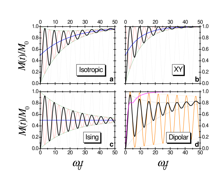
Figure 2.2: Temporal evolution of the polarization in the two-spin system interacting with a spin-bath for different system-environment interactions. Panels a), b) and c) show the polarization curves for the isotropic, XY and Ising SE Interaction, where $p_{\mathrm{XY}}$ takes the values $1/2$, $1$ and $0$ respectively. The black line is the magnetization of the spin $S$ and the red line is the magnetization of $I_{1}$ for a ratio $\Gamma_{\mathrm{SE}}/\left(\omega_{0}\hbar\right)=0.1.$ The blue line is the temporal evolution of the mean magnetization at each site. The green lines show the coherence decays with respect to the mean magnetization evolution. Panel c) shows the evolution of the $S$ magnetization with a dipolar SE interaction for different values of the ratio $\Gamma_{\mathrm{SE}}/\left(\omega_{0}\hbar\right)$. The orange, black and magenta lines show the temporal evolution for the ratios $1$, $0.1$ and $0.01$ respectively.

shows typical curves for different SE interactions (black lines). The blue line is the temporal evolution of the total magnetization divided by two or equivalently the mean magnetization at each site. We see that the curves go to $M_{0}$ for long times manifesting that the system arrives to the equilibrium state $\hat{\sigma}_{\infty}$ with the exception of the Ising SE interaction. In this case, the system has no injection from the spin-bath and goes to the quasi-equilibrium state of the $2$-spin system, i.e. the initial magnetization is spread over both sites. This quasi-equilibrium is described by

$$\hat{\sigma}^{\mathrm{qe}}=\frac{\exp\{-\widehat{\mathcal{H7}}_{\mathrm{S}}/(k_{\mathrm{B}}T_{\mathrm{qe}})\}}{\mathrm{Tr}\{\exp\{-\widehat{\mathcal{H}}_{\mathrm{S}}/(k_{\mathrm{B}}T_{\mathrm{qe}})\}\}}$$ (2.63)

with

$$T_{\mathrm{qe}}=2(\Omega_{1,I}/\Omega_{0,I})T.$$ (2.64)

In general, there is a competition between the Ising and the XY SE interaction terms that leads the system to a $2$-spin quasi-equilibrium state or to the total system equilibrium state respectively [CÁL⁺03, ÁLP07]. This quasi-equilibrium is time dependent and is given by the mean magnetization, $M_{\mathrm{tot}}\left(t\right)/2$, represented by the blue line in fig. 2.2. The green lines in the figure show the coherence decay relative to the mean magnetization at each site. We see that the XY interaction is the most coherent because its decoherence rate is equal to the magnetization transfer rate, while in the other cases, decoherence is faster than magnetization transfer. The red lines show the magnetization on the spin $I_{1}$ described by the expression

$$M_{I^{z}}\left(t\right)=M_{0}\left[1-\frac{1}{2}e^{-p_{\mathrm{XY}}\Gamma_{\mathrm{SE}}t/\hbar}+\frac{1}{2}e^{-\frac{1}{2}\left(1+p_{\mathrm{XY}}\right)\Gamma_{\mathrm{SE}}t/\hbar}\cos\left(\omega_{0}t\right)\right],$$ (2.65)

where only the sign of the oscillatory term $\operatorname{Re}\left\{\sigma_{32}\left(t\right)\right\}$ changes. Figure 2.2 c) shows curves with dipolar SE interaction for different values of the ratio $\Gamma_{\mathrm{SE}}/\left(\omega_{0}\hbar\right).$ It shows how the decoherence and magnetization transfer are stronger as $\Gamma_{\mathrm{SE}}/\left(\omega_{0}\hbar\right)$ becomes higher. Here, we observe the decoherence’s role described in the Introduction. The temporal interference pattern is described by the oscillatory term which contains the entangled two-spin superposition. A strong SE interaction leads to an efficient degradation of the two-spin quantum entanglement. This drives the system to a mixed-state, described by the diagonal elements of the density matrix, which constitutes the quasi-equilibrium state represented by the blue line. When decoherence is not too strong, we observe that it is not necessary to wait long times to obtain the maximum magnetization at the spin $S$ (totally polarized). It is enough to wait for a maximum of the oscillation at time $\pi/\omega_{0}$ where the magnetization reaches a value close to the maximum obtainable ($M_{0}$). But a more important result is that for an XY SE interaction, one can achieve the biggest gain of polarization at the first maximum of the oscillation. This is a consequence of the different behavior of the decoherent processes arising on the Ising or XY interactions. Moreover, for an XY SE interaction, expression (2.58) yields all the maxima of the oscillation equal to $M_{0},$regardless of the magnitude of the SE interaction. However, we should not forget that this expression is valid only for $\Gamma_{\mathrm{ZZ}},\Gamma_{\mathrm{XY}}\ll b$.

2.1.2.2 Non-secular solution

If we release the condition $\Gamma_{\mathrm{ZZ}},~{}\Gamma_{\mathrm{XY}}\ll b,$ i.e. we do not neglect the non-secular terms for the superoperator $\widehat{\widehat{\Gamma}}$, the dynamics still occurs in the Liouville space of the populations and ZQT. The solution of the generalized quantum master equation is now,

$$M_{S^{z}}\left(t\right)=M_{0}\left(1-a_{0}e^{-R_{0}t}-a_{1}\cos\left[\left(\omega+\mathrm{i}\eta\right)t+\phi_{0}\right]e^{-R_{1}t}\right),$$ (2.66)

where the real functions $\omega,$ $R_{0},R_{1}$ and $\eta$ as well as $a_{0}$, $a_{1}$ and $\phi_{0}$ depend exclusively on $b,$ $1/\tau_{\mathrm{SE}}=2\left(\Gamma_{\mathrm{ZZ}}+\Gamma_{\mathrm{XY}}\right)/\hbar$ and $p_{\mathrm{XY}}=\Gamma_{\mathrm{XY}}/\left(\Gamma_{\mathrm{ZZ}}+\Gamma_{\mathrm{XY}}\right)$. This expression will be discussed in chapter 3, where it is obtained from a microscopic derivation. However, it is important to remark that the short time evolution, $t\ll\tau_{\mathrm{SE}},$ of the secular expression does not satisfy the correct quadratic quantum behavior while the non-secular expression does. The relevance of this inertial property reflected in the quadratic short time evolution will become evident in chapter 4. We will see how it leads to the manifestation of something that we called an environmentally induced quantum dynamical phase transition [ÁDLP06, DÁLP07].

2.2 Three-spin quantum dynamics

In this section, we analyze theoretically and experimentally the quantum dynamics of a three-spin system coupled to a spin-bath during cross-polarization (CP) [HH62, MKBE74]. Our analysis takes into account a pure Hamiltonian behavior for a carbon ¹³C coupled to two protons ¹H, while the coupling to a spin-bath is treated in the fast fluctuation approximation. This model is inspired and then applied to the methylene and biphenyl groups of the smectic and nematic phases of the liquid crystal $4$-n-octyl-$4$’-cyanobiphenyl ($8$CB). We make use of the Hartmann-Hahn CP technique as a function of contact time to measure ¹H-¹³C and ¹H-¹H effective dipolar interactions. This technique has proved very useful in order to evaluate order parameters in liquid crystals [PR96]. Most of the previous works where transient oscillations were observed during CP were analyzed in terms of a single ¹H-¹³C interaction incorporating the interaction with other protons as a thermal bath or reservoir in a phenomenological way. However, many liquid crystals have alkyl chains and aromatic groups in their structures, where the carbon is coupled to more than one proton and the carbon-proton and proton-proton dipolar interactions are of the same order of magnitude. This led us to consider a set of three strongly dipolar coupled spins $1/2$ as the main system, which in turns interacts with the protons of the bath. Combining detailed calculations of the three-spin dynamics with structural information which provide the relative sign of the ¹H-¹³C couplings, we are able to obtain separately the ¹H-¹³C and ¹H-¹H effective interactions. In order to test the suitability of the formula obtained, we compare the values of the ¹H-¹³C couplings obtained by two procedures. One involves fitting of the data from a standard CP experiment to the calculated dynamics while in the other the ¹H-¹³C couplings are obtained directly from a CP under Lee-Goldburg conditions, i.e. when the dipolar proton-proton interactions have been cancelled out. The advantages and disadvantages of each procedure are discussed.

An interesting aspect we could observe during the CP dynamics in $8$CB is that the rate of attenuation of the oscillations (representing the coherences) is much faster than that of the polarization transfer from the bath in a factor several times larger than the one calculated assuming isotropic interaction with the bath [MKBE74]. We analyze here, the origin of this highly anisotropic behavior, not observed in solid molecular crystals [LUP98, HH94]. A well differentiated relaxation behavior among the two phases seems to indicate that while the extreme narrowing approximation is appropriate for the nematic phase, the description of the smectic phase requires the consideration of the slow motion limit.

2.2.1 An isolated three-spin system

We will consider the quantum evolution of a system of three spins $1/2$ coupled through the magnetic dipolar interaction during the contact time in a cross-polarization experiment [HH62, MKBE74]. The system is constituted by one spin $S$ and two spins $I$ representing a carbon-$13$ and two protons, respectively, under the presence of a static magnetic field $H_{0}$ in the $z$ direction and radio-frequency (RF) magnetic fields $H_{1,I}$ and $H_{1,S}$ in the $x$ direction. The Hamiltonian including the dipolar interactions truncated with respect to the Zeeman field $H_{0}$ and in a double rotating frame [Sli92] can be written as

$$\widehat{\mathcal{H}}_{\mathrm{S}}=\hbar\Delta\Omega_{I}\hat{I}^{z}+\hbar\Delta\Omega_{S}\hat{S}^{z}-\hbar\Omega_{1,I}\hat{I}^{x}-\hbar\Omega_{1,S}\hat{S}^{x}+2\sum_{k=1,2}b_{k}\hat{S}^{z}\hat{I}_{k}^{z}+d(2\hat{I}_{1}^{z}\hat{I}_{2}^{z}-\hat{I}_{1}^{x}\hat{I}_{2}^{x}-\hat{I}_{1}^{y}\hat{I}_{2}^{y}),$$ (2.67)

where, as in the previous section,

$$\Delta\Omega_{I}=\Omega_{0,I}-\omega_{\mathrm{rf},I}\;\;\;\;\;\text{and}\;\;\;\;\;\Delta\Omega_{S}=\Omega_{0,S}-\omega_{\mathrm{rf},S}$$ (2.68)

are the resonance offsets,

$$\hat{I}^{u}=\hat{I}_{1}^{u}+\hat{I}_{2}^{u}$$ (2.69)

with $\,u=x,y,z$,

$$\Omega_{1,I}=\gamma_{I}H_{1,I}\;\;\;\;\;\text{and}\;\;\;\;\;\Omega_{1,S}=\gamma_{S}H_{1,S}$$ (2.70)

where $\gamma_{I},\gamma_{S}$ are the gyromagnetic factors of the $I$ and $S$ spins. The constant, as defined in eq. (2.5),

$$b_{k}=-\frac{1}{2}\frac{\mu_{0}\gamma_{I}\gamma_{S}\hbar^{2}}{4\pi}\left\langle\frac{(3\cos^{2}(\theta_{Sk})-1)}{r_{Sk}^{3}}\right\rangle\qquad k=1,2$$ (2.71)

and

$$d=-\frac{1}{2}\frac{\mu_{0}\gamma_{I}^{2}\hbar^{2}}{4\pi}\left\langle\frac{(3\cos^{2}(\theta_{12})-1)}{r_{12}^{3}}\right\rangle$$ (2.72)

are the heteronuclear and homonuclear effective dipolar couplings respectively. However, here the angular brackets in the equations indicate that the dipolar couplings in liquid crystals are averaged over both molecular tumbling and any internal bond rotations. Thus, the molecular variation of the spin-spin distance, $r_{ij},$ and the angle between the internuclear vector and the external field, $\theta_{ij},$ are taken into account. Because of a special geometry of the oriented $n$CB liquid crystals, we will consider two different cases where the dipolar constants are related by $b_{1}=b_{2}=b$ and $b_{1}=-b_{2}=b.$

As in the previous section, for a standard CP experiment, one can neglect the resonance offsets, and considering that

$$|\Omega_{1,I}+\Omega_{1,S}|\gg|b_{k}|,|d|,$$ (2.73)

the truncated Hamiltonian can be written as

$$\widehat{\mathcal{H}}_{\mathrm{S}}=\tfrac{1}{2}\Sigma\left(\hat{S}^{x}+\hat{I}^{x}\right)+\tfrac{1}{2}\Delta\left(\hat{I}^{x}-\hat{S}^{x}\right)+\sum_{k=1,2}b_{k}\left(\hat{S}^{z}\hat{I}_{k}^{z}+\hat{S}^{y}\hat{I}_{k}^{y}\right)-\tfrac{1}{2}d(2\hat{I}_{1}^{x}\hat{I}_{2}^{x}-\hat{I}_{1}^{z}\hat{I}_{2}^{z}-\hat{I}_{1}^{y}\hat{I}_{2}^{y}),$$ (2.74)

with

$$\Sigma=-\hbar\left(\Omega_{1,S}+\Omega_{1,I}\right)\;\;\;\;\;\text{and}\;\;\;\;\;\Delta=\hbar\left(\Omega_{1,S}-\Omega_{1,I}\right).$$ (2.75)

As the Hamiltonian (2.74) has only Zeeman fields along the $x$ direction, we change the names of the axis as we did in section § 2.1.1: $x\rightarrow z,$ $y\rightarrow x$ and $z\rightarrow y.$ Hence, the Hamiltonian becomes

$$\widehat{\mathcal{H}}_{\mathrm{S}}=\tfrac{1}{2}\Sigma\left(\hat{S}^{z}+\hat{I}^{z}\right)+\tfrac{1}{2}\Delta\left(\hat{I}^{z}-\hat{S}^{z}\right)+\sum_{k=1,2}b_{k}\left(\hat{S}^{x}\hat{I}_{k}^{x}+\hat{S}^{y}\hat{I}_{k}^{y}\right)-\tfrac{1}{2}d(2\hat{I}_{1}^{z}\hat{I}_{2}^{z}-\hat{I}_{1}^{x}\hat{I}_{2}^{x}-\hat{I}_{1}^{y}\hat{I}_{2}^{y}).$$ (2.76)

In eq. (2.76) the non-secular elements of the dipolar interaction with respect to the $\Sigma\left(\hat{I}^{z}+\hat{S}^{z}\right)$ term have been neglected. Similar as in the previous section, this allows us to write the matrix representation of the Hamiltonian in a simple block structure using the basis $\left\{|M_{I},M_{S}\rangle\right\}$, with $M_{I}=M_{1}+M_{2}$ and $M_{S}$ denoting the spin projections of the $I$ and $S$ systems in the direction of their respective RF fields. Now, each block is characterized by the total spin projection $M=M_{I}+M_{S},$ i.e. nonzero matrix elements exist only between states with the same magnetic quantum numbers $M$. Thus, the heteronuclear dipolar Hamiltonian has non-diagonal terms different from zero generating transitions between spin states $\left\{|M_{I},M_{S}\rangle\right\}$ and $\left\{|M_{I}\pm 1,M_{S}\mp 1\rangle\right\}.$ The eigenstates of this Hamiltonian can be denoted in the form $|M,n_{M}\rangle$, with $n_{M}=1,..,g_{M}$, where $g_{M}$ is the degeneracy of $M$ ($n_{\pm 3/2}=1$ and  $n_{\pm 1/2}=1,2,3$). It is very interesting to note that in each space of $M=\pm 1/2$ there are only two of the three eigenstates that are involved in the dipolar transitions that give rise to the oscillations. This is a consequence of the symmetry of the system, i.e. the flip-flop can occur only between the carbon and one (the symmetric or the antisymmetric) combination of the proton states depending on the relative signs of the heteronuclear couplings ($b_{1}=b_{2}$ or $b_{1}=-b_{2}$). The symmetric and antisymmetric combination of the proton are

$$\left|S\right\rangle =1/\sqrt{2}\left(\left|+,-\right\rangle+\left|-,+\right\rangle\right),$$ (2.77)

$$\left|A\right\rangle =1/\sqrt{2}\left(\left|+,-\right\rangle-\left|-,+\right\rangle\right),$$ (2.78)

where the vectors are denoted by $\left|M_{1},M_{2}\right\rangle.$ Hence, in the ordered basis

$$\left\{\left|S\right\rangle\otimes\left|+\right\rangle;\left|+,+\right\rangle\otimes\left|-\right\rangle;\left|A\right\rangle\otimes\left|+\right\rangle\right\}$$ (2.79)

with $\left|M_{1},M_{2}\right\rangle\otimes\left|M_{S}\right\rangle$, the $M=1/2$ block of the system Hamiltonian is given by

$$\mathcal{H}_{\mathrm{S},M=\frac{1}{2}}=\left[\begin{array}[c]{ccc}\frac{1}{4}\left(\Sigma-\Delta\right)+\frac{1}{2}d&\frac{\sqrt{2}}{8}\left(b_{1}+b_{2}\right)&0\\ \frac{\sqrt{2}}{8}\left(b_{1}+b_{2}\right)&\left(\frac{1}{4}\Sigma+\frac{3}{4}\Delta\right)-\frac{1}{4}d&\frac{\sqrt{2}}{8}\left(b_{2}-b_{1}\right)\\ 0&\frac{\sqrt{2}}{8}\left(b_{2}-b_{1}\right)&\frac{1}{4}\left(\Sigma-\Delta\right)\end{array}\right],$$ (2.80)

and similarly for the $M=-1/2$ block. It is evident from the previous equation that under the conditions $b_{1}=b_{2}$ or $b_{1}=-b_{2}$ one of the states, the symmetric or antisymmetric, is involved in the dipolar transition.

The Liouville-von Neumann equation [Abr61, EBW91] for the density matrix of the system is (2.13)

$$\frac{\mathrm{d}}{\mathrm{d}t}\hat{\rho}\left(t\right)=-\frac{\mathrm{i}}{\hbar}[\widehat{\mathcal{H}}_{\mathrm{S}},\hat{\rho}\left(t\right)],$$ (2.81)

where, similarly as in the $2$-spin case (2.18), the initial density operator $\hat{\rho}(0)$ considering the situation after the $\pi/2$ pulse in the $I$ system is given by

$$\hat{\rho}\left(0\right)=\frac{\hat{1}+\beta_{\mathrm{B}}\hbar\Omega_{0,I}\hat{I}^{z}}{\mathrm{Tr}\left\{\hat{1}\right\}}.$$ (2.82)

The solution of this equation is given by

$$\rho(t)=\hat{U}(t)\rho(0)\hat{U}^{-1}(t),$$ (2.83)

where $\hat{U}(t)=\exp\left(-\frac{\mathrm{i}}{{}^{\hbar}}\widehat{\mathcal{H}}_{\mathrm{S}}t\right)$.

In the simplest case, where the Hartmann-Hahn condition is exactly fulfilled, $\Delta=0$, the exact solution for the evolution of the observed magnetization $M_{S^{z}}(t)$ is

$$M_{S^{z}}(t)=\mathrm{Tr}\left\{\hat{S}^{z}\hat{\sigma}\left(t\right)\right\}=M_{0}~{}f~{}\frac{\left[1-\cos(\omega_{0}t)\right]}{2},$$ (2.84)

where

$$\omega_{0}=\sqrt{\left(\frac{\kappa}{4}\right)^{2}\left(\frac{d}{\hbar}\right)^{2}+2\left(\frac{b}{\hbar}\right)^{2}}\text{\qquad and}\qquad f=2\left(\frac{b}{\hbar}\right)^{2}/\omega_{0}^{2}$$ (2.85)

with

$$\kappa=\left\{\begin{array}[c]{l}1\quad\text{if }b_{1}=-b_{2}=b\\ 3\quad\text{if }b_{1}=b_{2}=b\end{array}\right..$$ (2.86)

The natural frequency $\omega_{0}$ of the polarization transfer corresponds to the transitions between the eigenstates mentioned above. Now, it is clear that the symmetry of the system manifests directly in the frequency, where the difference between the two situations is represented through the $\kappa$ parameter. So, the relative signs of the heteronuclear couplings lead to a characteristic contribution of the homonuclear coupling being three times bigger when $b_{1}=b_{2}$ than when $b_{1}=-b_{2}$. The constant

$$M_{0}=\beta_{\mathrm{B}}\hbar\Omega_{0,I}/4$$ (2.87)

corresponds to the initial magnetization of one $I$ spin. Eq. (2.84) shows that the magnetization of $S$ is attenuated by the factor $f$, and it takes its maximum value $M_{0}$ when $d=0$, i.e. when there is no $I_{1}-I_{2}$ interaction. The fact that the homonuclear interaction decreases the transferred magnetization was already noticed in ref. [PUL96]. We can see that the constant term in eq. (2.84) is proportional to the differences in populations between the relevant eigenstates of the system, while the time dependent term corresponds to the coherences representing the transitions from $\left\{|M_{I},M_{S}\rangle\right\}$ to $\left\{|M_{I}\pm 1,M_{S}\mp 1\rangle\right\}$. The magnetization in the spins $I_{1}$ and $I_{2}$ is given by

$$\left.\begin{array}[c]{c}M_{I_{1}^{z}}\left(t\right)=\mathrm{Tr}\left\{\hat{I}_{1}^{z}\hat{\sigma}\left(t\right)\right\}\\ M_{I_{2}^{z}}\left(t\right)=\mathrm{Tr}\left\{\hat{I}_{2}^{z}\hat{\sigma}\left(t\right)\right\}\end{array}\right\}=M_{I^{z}}\left(t\right)=M_{0}\left\{1-\frac{1}{2}~{}f~{}\frac{\left[1-\cos\left(\omega_{0}t\right)\right]}{2}\right\}=M_{0}-\frac{1}{2}M_{S^{z}}\left(t\right)$$ (2.88)

and the total magnetization by

$$M_{\mathrm{tot}}\left(t\right)=\mathrm{Tr}\left\{\left(\hat{S}^{z}+\hat{I}_{1}^{z}+\hat{I}_{2}^{z}\right)\hat{\sigma}\left(t\right)\right\}=2M_{0}.$$ (2.89)

Thus, the total magnetization is given by the initial state and the mean magnetization in each site is given by $M_{\mathrm{tot}}\left(t\right)/3=\frac{2}{3}M_{0}.$ Because of the symmetry of the system, each of the proton transfers forth and back the same polarization to the carbon-$13$ that is half magnitude of the magnetization observed at site $S.$ Figure 2.3

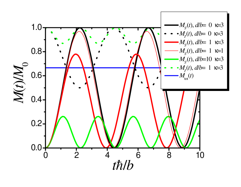
Figure 2.3: Temporal evolution of the polarization in a $3$-spin system. The black, red and blue lines are the $S$ (solid) and $I$ (dotted) magnetization with $b_{1}=b_{2}=b$ ($\kappa=3$) under the ratio $d/b=0,1$ and $10$ respectively. The thin red line represents the $S$ magnetization with $d/b=1$ and $b_{1}=-b_{2}=b$ $\left(\kappa=1\right).$ The blue line is the mean magnetization at each site $M_{\mathrm{tot}}\left(t\right)/3=2/3M_{0}.$

shows typical curves of the $M_{S^{z}}\left(t\right)$ and $M_{I^{z}}\left(t\right)$ magnetization. There, we can see curves for different values of the ratio $d/b,$ i.e. different factors $f.$ (the higher the ratio $d/b$, the lower the value of $f$). The red lines show the difference, with the same values of $b$ and $d,$ between the evolution with $b_{1}=b_{2}$ (solid line) and $b_{1}=-b_{2}$ (dashed line). The mean magnetization at each site is show by the blue line.

2.2.2 A three-spin system coupled to a spin-bath

In this section, we add to the three-spin system some interaction with other spins using an extension of the model proposed by Müller et al. [MKBE74], see section § 2.1.2. The model assumes that the dipolar interactions of the $S$ spin with the $I$ spins are neglected except for the coupling to $I_{1}$ and $I_{2}$. The interaction of these particular spins with the bath or the infinite reservoir of $I$ spins is considered in a phenomenological way. All kind of spin-lattice relaxations are neglected. The system-environment (SE) interaction Hamiltonian can be represented by

$$\widehat{\mathcal{H}}_{\mathrm{SE}} =\sum_{k=1,2}\left[\alpha\hat{I}_{k}^{z}\hat{F}_{k}^{z}+\beta\left(\hat{I}_{k}^{x}\hat{F}_{k}^{x}+\hat{I}_{k}^{y}\hat{F}_{k}^{y}\right)\right]$$

$$=\sum_{k=1,2}\left[\alpha\hat{I}_{k}^{0}\hat{F}_{k}^{0}+\tfrac{1}{2}\beta\left(\hat{I}_{k}^{-}\hat{F}_{k}^{+}+\hat{I}_{k}^{+}\hat{F}_{k}^{-}\right)\right]$$ (2.90)

with

$$\hat{F}_{k}^{u}=\sum_{l>2}d_{kl}I_{l}^{u},~{}~{}u=x,y,z$$ (2.91)

and

$$\hat{F}_{k}^{\pm}=\left(\hat{F}_{k}^{x}\pm\mathrm{i}\hat{F}_{k}^{y}\right)\text{ \ \ \ \ \ \ \ \ \ \ \ \ }\hat{F}_{k}^{0}=\hat{F}_{k}^{z}$$ (2.92)

where the subscript $l$ corresponds to the spins within the bath. As in section § 2.1.2, $\widehat{\mathcal{H}}_{\mathrm{SE}}$ is an Ising interaction if $\beta/\alpha=0$ and a XY, isotropic (Heisenberg) or the truncated dipolar interaction if $\alpha/\beta=0,1,-2$ respectively. Following the procedure of section § 2.1.2, in the semi-classical theory by tracing on the bath variables, $\hat{F}_{k}^{u}$ are treated as temporal functions $F_{k}^{u}\left(t\right)$ representing classical random processes. However, the NMR experimental conditions justify a high temperature approximation, and hence the semiclassical theory coincides with a quantum treatment [Abr61]. Then, the random SE interaction Hamiltonian is written as

$$\widehat{\mathcal{H}}_{\mathrm{SE}}\left(t\right)=\sum_{k=1,2}\left[\alpha F_{k}^{z}\left(t\right)\hat{I}_{k}^{z}+\tfrac{1}{2}\beta\left(F_{k}^{x}\left(t\right)\hat{I}_{k}^{x}+F_{k}^{y}\left(t\right)\hat{I}_{k}^{y}\right)\right].$$ (2.93)

 Here, the interaction of the system with the spins of the bath has been taken into account. Any influence of the bath coming from others degrees of freedom (rotations, translations, etc.) will manifest through this interaction. These random processes satisfy

$$\overline{F_{k}^{u}\left(t\right)}=0$$ (2.94)

where the bar denotes time average, and their correlation functions are

$$g_{k}^{\left(u,v\right)}\left(\tau\right)=\overline{F_{k}^{u}\left(t\right)F_{k}^{\nu\ast}\left(t+\tau\right)}.$$ (2.95)

 The dynamics of the reduced density operator $\hat{\sigma}\left(t\right)$, following the usual treatment to second order approximation, is [Abr61, Blu81, EBW91]

$$\frac{\mathrm{d}}{\mathrm{d}t}\hat{\sigma}\left(t\right)=-\frac{\mathrm{i}}{\hbar}[\widehat{\mathcal{H}}_{\mathrm{S}},\hat{\sigma}\left(t\right)]-\frac{1}{\hbar}\widehat{\widehat{\Gamma}}\left\{\hat{\sigma}\left(t\right)-\hat{\sigma}_{\infty}\right\}.$$ (2.96)

The relaxation superoperator $\widehat{\widehat{\Gamma}}$ generated by $\widehat{\mathcal{H}}_{\mathrm{SE}}\left(t\right)$, that accounts for the dissipative interactions between the reduced spin system and the bath, drives the density operator towards its equilibrium value $\hat{\sigma}_{\infty}$.

In the following, we assume that the correlation times of the fluctuations are extremely short compared with all the relevant transitions rates between eigenstates of the Hamiltonian, i.e. frequencies of the order of $\Sigma/2$ and $\omega_{0}$. In this extreme narrowing regime we obtain

$$\widehat{\widehat{\Gamma}}\left\{\hat{\sigma}\right\}=\frac{1}{2}\sum_{k}\sum_{u,v}\xi_{u,v}\mathcal{J}_{k}^{\left(u,v\right)}\left(0\right)\left[\hat{I}_{k}^{u},\left[\hat{I}_{k}^{\nu},\hat{\sigma}\right]\right],$$

where

$$\mathcal{J}_{k}^{\left(u,v\right)}\left(\omega\right)=\int_{-\infty}^{\infty}\frac{d\tau}{\hbar}g_{k}^{\left(u,v\right)}\left(\tau\right)\exp\left\{-\mathrm{i}\omega\tau\right\}$$ (2.97)

is the spectral density and

$$\xi_{u,v}=\left(\alpha\delta_{u,z}+\beta\left(\delta_{u,x}+\delta_{u,y}\right)\right)\left(\alpha\delta_{v,z}+\beta\left(\delta_{v,x}+\delta_{v,y}\right)\right).$$ (2.98)

If we suppose the spatial directions statistically independent, i.e.

$$g_{k}^{\left(u,v\right)}\left(\tau\right)=0\;\;\;\;\;\text{if}\;\;u\neq v,$$ (2.99)

the superoperator $\widehat{\widehat{\Gamma}}$ can be written as

$$\widehat{\widehat{\Gamma}}\left\{\hat{\sigma}\right\}=\sum_{k=1,2}\alpha^{2}\mathcal{J}_{k}^{z}\left[\hat{I}_{k}^{z},\left[\hat{I}_{k}^{z},\hat{\sigma}\right]\right]+\beta^{2}\mathcal{J}_{k}^{x}\left[\hat{I}_{k}^{x},\left[\hat{I}_{k}^{x},\hat{\sigma}\right]\right]+\beta^{2}\mathcal{J}_{k}^{y}\left[\hat{I}_{k}^{y},\left[\hat{I}_{k}^{y},\hat{\sigma}\right]\right],$$ (2.100)

where

$$\mathcal{J}_{k}^{u}=\frac{1}{2}\mathcal{J}_{k}^{\left(u,u\right)}\left(0\right).$$ (2.101)

Here, as in the two-spin case, the axial symmetry of $\widehat{\mathcal{H}}_{\mathrm{S}}$ around the $z$ axis leads to the impossibility to evaluate separately $\mathcal{J}_{k}^{x}$ and $\mathcal{J}_{k}^{y}$, so they will appear only as the averaged value

$$\mathcal{J}_{k}^{xy}=\left(\mathcal{J}_{k}^{x}+\mathcal{J}_{k}^{y}\right)/2.$$ (2.102)

Taking into account the symmetry of our system $b_{1}=\pm b_{2}$, an extra simplification can be done by

$$\mathcal{J}^{u}=\left(\mathcal{J}_{1}^{u}+\mathcal{J}_{2}^{u}\right)/2.$$ (2.103)

Thus, we obtain

$$\widehat{\widehat{\Gamma}}\left\{\hat{\sigma}\right\}=\sum_{k=1,2}\alpha^{2}\mathcal{J}^{z}\left[\hat{I}_{k}^{z},\left[\hat{I}_{k}^{z},\hat{\sigma}\right]\right]+\beta^{2}\mathcal{J}^{xy}\left(\left[\hat{I}_{k}^{x},\left[\hat{I}_{k}^{x},\hat{\sigma}\right]\right]+\left[\hat{I}_{k}^{y},\left[\hat{I}_{k}^{y},\hat{\sigma}\right]\right]\right).$$ (2.104)

Although we could absorb the constant $\alpha^{2}$ and $\beta^{2}$ in $\mathcal{J}^{z}$ and $\mathcal{J}^{xy}$ respectively, we will keep it to emphasize the different sources of the anisotropy in eq. (2.104). As we discuss in section § 2.1.2, the most usual approximation is to consider $\mathcal{J}^{x}=\mathcal{J}^{y}=\mathcal{J}^{z}$ (identical correlations in all the spatial directions) and $\alpha=\beta=1$ (isotropic interaction Hamiltonian) [MKBE74], however, a better approximation considers a dipolar interaction Hamiltonian, i.e. $\alpha=-2\beta=-2.$ As in eq. (2.47), we define

$$\Gamma_{\mathrm{ZZ}}=\alpha^{2}\mathcal{J}^{z}\;\;\;\;\;\text{and}\;\;\;\;\;\Gamma_{\mathrm{XY}}=\beta^{2}\mathcal{J}^{xy}.$$ (2.105)

2.2.2.1 Neglecting non-secular terms

Following the formalism in Abragam and Ernst et al. books [Abr61, EBW91] that was used in section § 2.1.2.1, we write the superoperator $\widehat{\widehat{\Gamma}}$ using the basis of eigenstates of the Hamiltonian (2.74). After neglecting the rapidly oscillating non-secular terms with respect to the Hamiltonian, i.e., $\Gamma_{\mathrm{XY}},\Gamma_{\mathrm{ZZ}}\ll\left|b\right|,\left|d\right|$, a block structure results. The first block couples the populations and off-diagonal elements with $\Delta M=0$, Zero Quantum Transitions (ZQT), of the density matrix. Each of the following blocks couples one order $\Delta M\geq 1$ of off-diagonal elements of the density matrix among themselves. Because the Hamiltonian (2.74) does not have degenerate eigenenergies, all the non-diagonal terms coupling the population block with the ZQT block are non-secular and can be neglected. As the initial condition (2.82) does not contain coherences with $\Delta M\geq 1,$ we only need to study the evolution of the density operator into a Liouville space restricted to populations and ZQT. When there are no degenerate transitions, the secular ZQT block is diagonal. However, in our case there are degenerate transitions between eigenstates within the sets with $M=\pm 1/2.$ Thus, some non-diagonal terms in the ZQT block cannot be neglected.

In the final condition, the $SI_{2}$ system reaches the temperature of the $I$ spins reservoir as was described in the section § 2.1.2:

$$\hat{\sigma}_{\infty}=\frac{\hat{1}+\beta_{\mathrm{B}}\hbar\Omega_{0,I}\left(\hat{S}^{z}+\hat{I}^{z}\right)}{\mathrm{Tr}\left\{\hat{1}\right\}}.$$ (2.106)

It is easily seen that $\hat{\sigma}_{\infty}$ commutes with $\widehat{\mathcal{H}}_{\mathrm{S}}$, not containing coherences with $\Delta M\geq 1$.

By using the present formalism under the considered approximations, we will solve eq. (2.39) for the cases relevant to our liquid crystal study.

Isotropic system-environment interaction rate.

Considering

$$\Gamma_{\mathrm{ZZ}}=\Gamma_{\mathrm{XY}}=\Gamma\;\;\;~{}\ \;\;\;\;\ \;\;\;\ \ \ (\mathcal{J}^{z}=\mathcal{J}^{xy}\;\;\;\text{and\ \ \ }\alpha=\beta=1),$$ (2.107)

the time evolution of the $S$ magnetization results

$$M_{S^{z}}\left(t\right)=M_{0}\left[1-A_{+}e^{-R_{+}t}-A_{-}e^{-R_{-}t}-A_{\mathrm{c}}\cos\left(\omega t\right)\,e^{-R_{\mathrm{c}}t}\right],$$ (2.108)

where

$$\omega =\omega_{0},$$ (2.109)

$$R_{\pm} =\chi_{\pm}\Gamma/\hbar,$$ (2.110)

$$R_{\mathrm{c}} =\chi_{\mathrm{c}}\Gamma/\hbar,$$ (2.111)

with

$$\chi_{\pm} =1+\frac{5}{4}f\pm\sqrt{\left(\frac{5}{4}f-1\right)^{2}+f}$$ (2.112)

$$\chi_{\mathrm{c}} =3-\frac{5}{4}f$$ (2.113)

and

$$A_{\pm} =\frac{1}{2}\left\{\left(1-\frac{f}{2}\right)\pm\frac{\left[\frac{5}{4}f\left(1-\frac{f}{2}\right)-1\right]}{\sqrt{\left(\frac{5}{4}f-1\right)^{2}+f}}\right\}$$ (2.114)

$$A_{\mathrm{c}} =\frac{1}{2}f.$$ (2.115)

The figure 2.4

Figure 2.4: Typical curves of the magnetization of the $S$ spin in a three-spin system coupled to a spin-bath under an isotropic SE interaction. The thick red, black and green lines are the polarization evolution with $f=1$ and the ratios $\Gamma/\left(\omega_{0}\hbar\right)=0.01,$ $0.06$ and $0.2$ respectively. The black thin line represents the magnetization for $f=0.7$ and $\Gamma/\left(\omega_{0}\hbar\right)=0.06$ and the light and dark gray dotted lines are the isolated dynamics for $f=1$ and $0.7$ respectively.

shows typical curves of eq. (2.108) for different values of the ratio $\Gamma/\left(\omega_{0}\hbar\right).$ As we observed in the $2$-spin case, we see that the oscillations are attenuated when the ratio is bigger and the net transfer of polarization is faster. The black lines compare two different curves with $f=1$ (thick line) and $f=0.7$ (thin line) for a fixed value of $\Gamma/\left(\omega_{0}\hbar\right).$ We observe that the maximum of the oscillation is smaller as $f$ decreases but the final magnetization is the same for both curves. The figure 2.5

Figure 2.5: Coefficients $A_{i}$ [panel a)] and relaxation rates $R_{i}$ [panel b)] of the $S$ polarization expression (2.108) for an isotropic system-environment interaction as a function of the relation between homo and heteronuclear spin couplings $f$.

shows the dependence of the coefficients $A_{i}$ and the relaxation rates $R_{i}$ as a function of $f.$ Notice that $\chi_{\pm},\chi_{\mathrm{c}}\geq 0.$ Using the initial condition $M_{S^{z}}\left(0\right)=0,$ it is easy to see that the positive constants $A_{+},A_{-},$ $A_{\mathrm{c}}$ satisfy $1-A_{+}-A_{-}-A_{\mathrm{c}}=0$. In general $A_{+}\ll A_{-}$ and $R_{+}>R_{-}$, so the first exponential term can be neglected as can be observed in fig. 2.6.

Figure 2.6: Polarization evolution of the $S$ magnetization (black lines) of a $3$-spin system coupled to a spin-bath. The figure shows comparisons between $M_{S^{z}}\left(t\right)$ and the aproximate solution (red line) where was neglected one of the pure exponetial term. The pure exponetial terms that are contained in the $M_{S^{z}}\left(t\right)$ expression are showed by the blue and green line. It is evident why the term described by the green line could be neglected. The light gray line shows the isolated evolution of the $S$ magnetization to observe that the first maximun is essentially $fM_{0}$. Panel a) shows the evolution for $f=1$ and panel b) for $f=0.2$ where in the last one the aproximate solution is more better.

This approximate solution is excellent for $f\ll 1$, but even in the worst case ($f\sim 1$), it differs about $7\%$ from the exact solution (see fig. 2.6).

The first maximum in the magnetization $M_{S^{z}}\left(t\right)$ is approximately $f\,M_{0}$ and the oscillation has frequency $\omega_{0}$ as can be observed comparing with the isolated evolution in figs. 2.4 and 2.6. The oscillations have an amplitude $\frac{f}{2}e^{-R_{\mathrm{c}}t}$ that represents the attenuation of the coherences of the $SI_{2}$ system mounted over non-oscillatory terms. These terms take into account the effect of the bath, not only by transferring magnetization but also breaking coherences and leading to a quasi-equilibrium. This quasi-equilibrium state is given by

$$\hat{\sigma}^{\mathrm{qe}}=\exp\{-\widehat{\mathcal{H7}}_{\mathrm{S}}/(k_{\mathrm{B}}T_{\mathrm{qe}})\}/\mathrm{Tr}\{\exp\{-\widehat{\mathcal{H}}_{\mathrm{S}}/(k_{\mathrm{B}}T_{\mathrm{qe}})\}\}$$ (2.116)

with

$$T_{\mathrm{qe}}=3/2(\Omega_{1,I}/\Omega_{0,I})T$$ (2.117)

the temperature of the three-spin system.

In the particular case when $f=1,$ i.e. no $I_{1}$-$I_{2}$ interaction, $A_{\pm}=\frac{1}{4}\left(1\mp\frac{3}{\sqrt{17}}\right)$, $A_{\mathrm{c}}=f/2,$ $R_{\pm}=\frac{1}{4}\left(9\pm\sqrt{17}\right)\Gamma/\hbar$ , $R_{\mathrm{c}}=7/4\Gamma/\hbar$ and $\omega_{0}=\sqrt{2}b/\hbar$, showing that only under this condition the frequency given in ref. [PR96] is valid. But even under this condition, our results show that the equation obtained by Müller et al. for the $SI$ case cannot be directly applied to the $SI_{2}$ system. In this last case the attenuation of the oscillations and the transfer of polarization to the system is slightly faster than in the $SI$ case.

Anisotropic system-environment interaction rate.

Considering

$$\Gamma_{\mathrm{ZZ}}\neq\Gamma_{\mathrm{XY}},$$ (2.118)

we obtain

$$M_{S^{z}}\left(t\right)=M_{0}\left[1-A_{1}e^{-R_{1}t}-A_{2}e^{-R_{2}t}-A_{3}e^{-R_{3}t}-A_{\mathrm{c}}\cos\left(\omega t\right)\,e^{-R_{\mathrm{c}}t}\right],$$ (2.119)

where the $A_{i},$ $i=1,2,3$ are functions of $f$ and $\Gamma_{\mathrm{ZZ}}/\Gamma_{\mathrm{XY}}$ and

$$\omega =\omega_{0},$$ (2.120)

$$R_{\mathrm{c}} =\left(2-f\right)\Gamma_{\mathrm{XY}}/\hbar+\left(1-\frac{1}{4}f\right)\Gamma_{\mathrm{ZZ}}/\hbar,$$ (2.121)

$$A_{\mathrm{c}} =\frac{1}{2}f.$$ (2.122)

The expressions for $A_{i}=A_{i}(f,\Gamma_{\mathrm{ZZ}}/\Gamma_{\mathrm{XY}})$ and $R_{i}=R_{i}(f,\Gamma_{\mathrm{ZZ}}/\hbar,\Gamma_{\mathrm{XY}}/\hbar)$ are too long to be included here but they are available as supplementary material.

The transfer of polarization from the bath to the system depends on the non-oscillatory terms of eq. (2.119). In the $\Gamma_{\mathrm{ZZ}}/\Gamma_{\mathrm{XY}}\geq 1$ case, at long times ($R_{\mathrm{c}}t>>1$), only one of the three exponential terms contributes. In this regime, the transfer is essentially given by $\Gamma_{\mathrm{XY}}$, although there is a slight dependence on $\Gamma_{\mathrm{ZZ}}$. This differs from the $SI$ behavior where the polarization transfer from the bath depends exclusively on $\Gamma_{\mathrm{XY}}$ (see section § 2.1.2). This is a consequence of the fact that in the $SI$ system the quasi-equilibrium $S^{z}$ polarization, $(1/2)M_{0}$ (the mean magnetization at each site), coincides with the time averaged value of the isolated system. As $\Gamma_{\mathrm{XY}}$ is associated to the flip-flop term in the SE interaction Hamiltonian (2.90), its role transferring polarization can be easily interpreted. The effect of $\Gamma_{\mathrm{ZZ}}$ is more subtle, it can be associated to a process where the environment observes the system breaking its coherences. This process that involves the operator $\hat{F}^{z}\hat{I}^{z}$ in $\widehat{\mathcal{H}}_{\mathrm{SE}},$ which is a like number operator, is discussed in chapter 3.

Figure 2.7

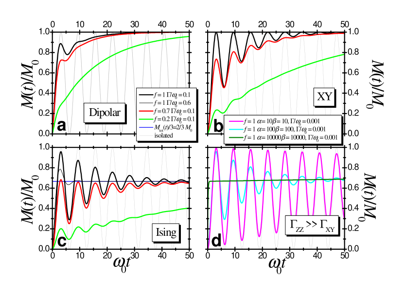
Figure 2.7: Typical curves of the $S$ polarization (2.119) for different SE interactions and values of $f$ (the relation between $b$ and $d$). The dipolar, XY and isotropic SE are showed in panel a), b) and c) respectively. In the limit $\Gamma_{\mathrm{ZZ}}\gg\Gamma_{\mathrm{XY}}$ [highly anisotropic case, panel d)] it is possible to distinguish two time regimes: one in which the system decoheres and reaches a quasi-equilibrium, $[\widehat{\mathcal{H}}_{\mathrm{S}},\hat{\sigma}^{\mathrm{qe}}]=0$, and other in which polarization transfer from the bath is completed with a rate $\Gamma_{\mathrm{XY}}/\hbar.$

shows typical curves of the $S$ polarization (2.119) for different SE interactions and values of $f$ (the relation between $b$ and $d$). In the limit $\Gamma_{\mathrm{ZZ}}\gg\Gamma_{\mathrm{XY}}$ [highly anisotropic case, panel d)] it is possible to distinguish two time regimes: one in which the system decoheres and reaches a quasi-equilibrium, $[\widehat{\mathcal{H}}_{\mathrm{S}},\hat{\sigma}^{\mathrm{qe}}]=0$ [SHE98], characterized by $\Gamma_{\mathrm{ZZ}}$ and other in which polarization transfer from the bath is completed with a rate $\Gamma_{\mathrm{XY}}/\hbar.$ In this situation, it is possible to see that $R_{\mathrm{c}}$ is proportional to $\Gamma_{\mathrm{ZZ}}$, as it occurs with the $R_{i}$ corresponding to the fastest exponential terms. The dependence of the non-oscillatory terms on $\Gamma_{\mathrm{ZZ}}$ observed in the $SI_{2}$ system can be assigned to the fact that the quasi-equilibrium carbon polarization $(2/3)M_{0}$ (the mean magnetization at each site) does not coincide with its time averaged value $(f/2)M_{0}$ in the isolated three-spin system [eq. (2.84)].

Equations (2.108) and (2.119) will be used to fit the experimental data in order to extract the relevant parameters of our system.

2.2.3 Many-spin quantum dynamics during Cross-Polarization in 8CB

Nuclear Magnetic Resonance experiments were carried out by people of our group in $4$-n-octyl-$4$’-cyanobiphenyl, also called $8$CB (see fig. 2.8) obtained from Sigma (Chemical, Co) and used without further purification. This system presents the mesophases smectic A (SA) and nematic (N), with transition temperatures at $294.5\operatorname{K}$ (K-SA), $306.5\operatorname{K}$ (SA-N) and $313.5\operatorname{K}$ (N-I).

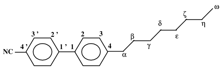
Figure 2.8: Chemical structure of $4$-n-octyl-$4$’-cyanobiphenyl ($8$CB) showing the labels used in the ¹³C-NMR spectra.

¹H-¹³C cross-polarization measurements as a function of contact time $t_{\mathrm{c}}$ were performed in the smectic and nematic mesophases. In all the cases, the CP sequence was performed in static conditions and combined with the sequence SPINAL-$64$ to perform an efficient proton decoupling during acquisition without appreciable heating of the sample [FKE00].

In the smectic phase, standard CP experiments were performed at $300\operatorname{K}$ in a Bruker MSL-$300$. The acquisition time was $92\operatorname{ms}$, with $60\operatorname{ms}$ for decoupling and a recycling time of $15\operatorname{s}$. The Hartmann-Hahn (H-H) condition [HH62, Sli92] was set with an RF field amplitude for carbons corresponding to $\Omega_{1,S}/2\pi=67.7\operatorname{kHz}$. During the experiment the contact time was varied in the range $2\operatorname{\mu s}$ $<t_{\mathrm{c}}<5\operatorname{ms}$.

In the nematic phase at $311.5\operatorname{K}$ two types of CP experiments were performed in a Bruker AVANCE DSX-$500$. The first was a standard CP with protons on-resonance. The second was a CP experiment with irradiation for protons in the Lee-Goldburg (LG) condition, i.e. the off-resonance for protons was set to have an effective field at the magic-angle with the static field $H_{0}$. The acquisition and decoupling times were $74\operatorname{ms}$. In the standard CP, the H-H condition was set with $\Omega_{1,S}/2\pi=60.3\operatorname{kHz}$ while in the Lee-Goldburg $\Omega_{1,S}/2\pi=74\operatorname{kHz}$. In both sets of experiments the H-H condition was optimized for $C(\gamma)$ (see figs. 2.8 and 2.9), and the contact time $t_{\mathrm{c}}$ varied up to $2\operatorname{ms}$.

Figure 2.9: ¹³C-NMR spectra of $8$CB in the smectic mesophase at $300\operatorname{K}$. In the inset we see the aliphatic part of the spectrum corresponding to $311.5{}\operatorname{K}$ (nematics), which is the only part that changes at the working temperatures. The assignments for the aliphatic part of the spectrum have been done in previous works. Labels refer to fig. 2.8.

In all these experiments the temperatures were calibrated using the N-I temperature transition. Also a ¹³C-NMR spectrum of $8$CB in the isotropic phase (at $320\operatorname{K}$) was taken as reference using a single pulse sequence with ¹H decoupling (direct ¹³C polarization).

2.2.3.1 Comparison between experiments and theoretical results

The ¹³C-NMR spectrum of $8$CB in smectic phase can be seen in fig. 2.9. In the inset of this figure, the alkyl part of the spectrum at a temperature corresponding to the nematic mesophase is displayed. The aromatic part of the spectrum keeps the same features up to the nematic-isotropic transition temperature. The position of C($\omega$), methyl group, which in the isotropic phase is at $14.1$ ppm has been taken as reference because, as experimentally observed, it does not vary at the working temperatures due to its high mobility. The aromatic part of the carbon spectrum for $8$CB is similar to those of other members of the $n$CB series, so we consider the up-dated assignments reported for $5$CB in previous works [FKE00]. A detailed temperature dependence of the ¹³C chemical shifts in $8$CB as well as their complete assignments have been reported previously [CCH⁺02]. The assignments for the alkyl carbons are supported by the segmental order parameters obtained from experimental CP frequencies (see below), and deuterium NMR experiments [Don97, CEHL85].

In order to analyze the experimental data, it is necessary to correlate the geometry/symmetry of the molecular interactions with the cases presented in the theoretical section associated to different values of $\kappa,$ eq. (2.86). For each methylene carbon in the aliphatic chain, the geometry of the molecule and the rapid rotations around the C-C bonds, which lead to the trans-gauche isomerizations, allows us to take a single averaged value for both heteronuclear couplings i.e. $b_{1}\approx$ $b_{2}$. Then, for carbons C($\alpha$) to C($\eta$) in the aliphatic chain the relation of signs of the heteronuclear couplings corresponds to the case where $\kappa=3$. It is also possible to see from simulations done with a similar molecule ($4$-n-pentyl-$4$’-cyanobiphenyl or $5$CB) and from geometrical considerations that the homonuclear dipolar interaction $d$ between protons belonging to the same methylene in general, cannot be neglected [SKSM01]. For each non-quaternary carbon in the phenyls rings C($3^{\prime}$), C($2^{\prime}$), C($2$) and C($3$), we have one directly bonded proton interacting with a dipolar coupling $b_{1}$; however, a careful analysis indicates that neither the ¹H-¹H interaction $d$ nor the coupling between the ¹³C and the nearest non-bonded ¹H, $b_{2},$ can be neglected. Considering the rigidity of the phenyl ring and the orientation of each internuclear vector with respect to the external field, we see that $b_{1}\approx-b_{2}.$ Then, each non-quaternary aromatic carbon is part of a three-spin system, where both heteronuclear couplings can be considered having an averaged magnitude $b=\sqrt{\left(b_{1}^{2}+b_{2}^{2}\right)/2}$ and different relative signs, leading to $\kappa=1$.

Firstly, let’s consider the experimental results corresponding to the smectic phase. In this case, typical oscillations and relaxation of the ¹³C polarization vs. contact time $t_{\mathrm{c}}$ are shown in fig. 2.10. We remark that neither the quaternary carbons nor C($\omega$) show oscillations in the CP experiment. In the last case, the reason is the high mobility of the methyl group that averages to zero the effective carbon-proton interaction. In all these experiments, the ¹³C polarization has essentially reached its asymptotic value at $5\operatorname{ms}$. The absence of a decay in these curves allows us to neglect spin-lattice relaxation in the rotating frame ($T_{1\rho}$) in the time regime analyzed. We also note that the CP frequencies corresponding to methylene groups are higher than those of the aromatic cores. This is due to a particularly unfavorable angle ($\sim 60^{\circ}$) between the internuclear carbon-proton vector and the external magnetic field in the case of the phenyl rings. Besides, the contribution of the homonuclear coupling to the frequency is much smaller when $\kappa=1$. In each dynamical curve shown in fig. 2.10, the ¹³C polarization at the first maximum is lower than its asymptotic value. As we have seen in the theoretical section, this fact indicates that the homonuclear coupling is not negligible and it will allow us to evaluate it.

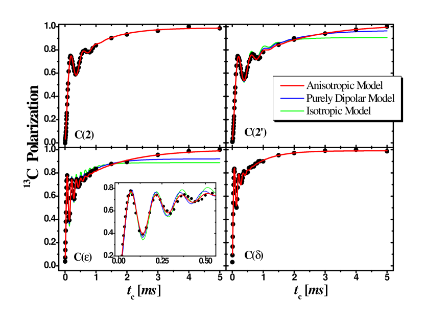
Figure 2.10: ¹³C polarization as a function of contact time $t_{\mathrm{c}}$ for aromatic and aliphatic carbons in a standard CP experiment at $300{}\operatorname{K}$ (smectic phase). Fittings of the experimental data to the anisotropic, isotropic and purely dipolar models described in the text, are displayed.

We have fitted the experimental CP data to the equations derived for the isotropic (eq. (2.108)) and anisotropic models (eq. (2.119)) presented in section § 2.2.2.1. In the last case, we have distinguished a purely dipolar anisotropy ($\alpha=-2\beta=-2$ and $\mathcal{J}^{xy}=\mathcal{J}^{z},$ i.e. $\Gamma_{\mathrm{ZZ}}/\Gamma_{\mathrm{XY}}=4$) from the most general case. For the smectic phase, it is seen in fig. 2.10 that the isotropic model separates from the experimental points after approximately the time of the second maximum, fitting very poorly the asymptotic behavior. The dipolar model constitutes an improvement over the isotropic one, without adding extra free parameters. However, a much better fitting is obtained using the anisotropic model which follows very closely the first oscillations of the magnetization and it is the best suited in the asymptotic regime.

In the case of the standard CP experiments performed in the nematic phase up to $2\operatorname{ms}$ (not shown in the figure), the behavior is already well fitted with the purely dipolar model, not showing any appreciable improvement by the use of the completely anisotropic model.

Taking into account the fitting parameters corresponding to each experiment, we can obtain the effective dipolar couplings and the relaxation constants for each carbon showing oscillations during CP. In tables 2.1 and 2.2, we show the heteronuclear and homonuclear dipolar couplings at different temperatures. The values for the heteronuclear couplings are comparables with those obtained for $8$CB in ref. [FPG⁺86], where a different experimental technique was applied.

Carbons $\begin{array}[c]{c}\frac{1}{2\pi}b/\hbar\\ \operatorname{kHz}\end{array}$ $\begin{array}[c]{c}\frac{1}{2\pi}d/\hbar\\ \operatorname{kHz}\end{array}$ C($3^{\prime}$) $1.30\pm 0.03$ $4.9\pm 0.3$ C($2^{\prime}$) $1.49\pm 0.04$ $4.8\pm 0.3$ C($2$) $1.58\pm 0.06$ $4.9\pm 0.3$ C($3$) $1.45\pm 0.04$ $5.3\pm 0.4$ C($\beta$) $4.6\pm 0.1$ $4.5\pm 0.6$ C($\gamma$) $4.8\pm 0.1$ $5.9\pm 0.7$ C($\delta$) $4.7\pm 0.3$ $2.9\pm 0.3$ C($\varepsilon$) $4.3\pm 0.2$ $4.0\pm 0.5$ C($\varsigma$) $3.1\pm 0.1$ $3.7\pm 0.4$ C($\eta$) $3.2\pm 0.1$ $2.2\pm 0.3$

Table 2.1: Effective heteronuclear and homonuclear dipolar couplings $b$ and $d$ obtained by fitting the data of the standard CP experiment performed at 300K (smectic phase) to the anisotropic model. The signal corresponding to C($\alpha$) does not appear in the smectic spectra. The errors have been assigned taking into account eqs. (2.123) for $b$, $d$ in terms of the fitted parameters.

Carbons $\begin{array}[c]{c}\text{Standard CP}\\ \frac{1}{2\pi}b/\hbar\\ \operatorname{kHz}\end{array}$ $\begin{array}[c]{c}\text{LG-CP}\\ \frac{1}{2\pi}b/\hbar\\ \operatorname{kHz}\end{array}$ $\begin{array}[c]{c}\text{Standard CP}\\ \frac{1}{2\pi}d/\hbar\\ \operatorname{kHz}\end{array}$ $\begin{array}[c]{c}\text{LG-CP}\\ \frac{1}{2\pi}d/\hbar\\ \operatorname{kHz}\end{array}$ C($\alpha$) $4.0\pm 0.2$ $4.18\pm 0.04$ $2.7\pm 0.5$ $2.9\pm 0.6$ C($\beta,\delta$) $2.7\pm 0.1$ $2.95\pm 0.03$ $3.5\pm 0.6$ $2.8\pm 0.6$ C($\gamma$) $3.0\pm 0.2$ $3.34\pm 0.03$ $3.5\pm 0.7$ $2.5\pm 0.5$ C($\varepsilon$) $2.8\pm 0.1$ $2.95\pm 0.03$ $3.1\pm 0.5$ $2.8\pm 0.6$ C($\varsigma$) $2.5\pm 0.1$ $2.29\pm 0.03$ $2.4\pm 0.5$ $2.8\pm 0.5$ C($\eta$) $2.4\pm 0.1$ $2.17\pm 0.03$ $1.5\pm 0.3$ $2.3\pm 0.4$

Table 2.2: Effective heteronuclear and homonuclear dipolar couplings $b$ and $d$ for the aliphatic carbons obtained from the experiments performed at 311.5K (nematic phase). In the standard CP experiment the values are obtained by fitting the data to the purely dipolar model (see text). In LG-CP the values of $b$ are obtained directly from eq. (2.124) while the values of $d$ requires a combination of the standard CP with the LG-CP frequencies (eq. (2.127)). In this mesophase the signal of C($\beta$) merges to the signal of C($\delta$), so the same value of coupling has been assigned for both carbons.

It is important to emphasize here, that the frequency of the oscillations $\omega$ is a quite independent and robust parameter, leading to values which vary less than $4\%$ using different models. This allows one to determine the heteronuclear coupling $b$ with very small error. The homonuclear coupling, however, is much more sensitive to the relation between the oscillatory and the asymptotic regimes and so, more dependent on the model and the extent of the experimental data. To see clearly this fact, we notice that the frequency and the attenuation factor $f$ given in eq. (2.85) are the fitting parameters that yield$\ b$ and $d$ regardless of the model. The dependence between these parameters and the couplings are

$$\frac{1}{2\pi}\frac{b}{\hbar}=\frac{1}{\sqrt{2}}\frac{\omega}{2\pi}\sqrt{f}\text{ \qquad and \qquad}\frac{1}{2\pi}\frac{d}{\hbar}=\frac{4}{\kappa}\frac{\omega}{2\pi}\sqrt{\left(1-f\right)}.$$ (2.123)

As in our cases, $f$ is always bigger than $1/2$, the error in $f$ (approx. $2\%$ for the experiment in smectic and $5\%$ for the experiment in nematics) affects less to $b$ than $d$. Now, taking into account that the CP frequency $\omega$ is the best parameter, fitted with an error lower than $2\%$, we can assign the error of the other parameters of interest. Then, the coupling $b$ is obtained with a relative error between $3\%$ and $5\%$ while the relative error of $d$ reaches in some cases a value of about $20\%$.

Fig. 2.11 displays the tendency of the CP frequency obtained for the different experiments. In particular, for the aliphatic carbons, the expected zig-zag pattern is observed [Don97, CEHL85]. For the aromatic part of the molecule we have $\omega(3^{\prime})\lessapprox\omega(2^{\prime})\approx\omega(2)\approx\omega(3)$, this is expected because C($3\prime$), being the closest to the cyano group forms a bigger C-C-H angle, giving rise to a smaller dipolar interaction [CHEP96]. On the other hand, when increasing temperature, i.e. going from smectic to nematic, a further averaging of the dipolar interactions occurs, manifested in the decrease of the CP frequencies. For comparison, fig. 2.11 shows the results of the CP experiment at the Lee-Goldburg condition, performed in the nematic phase at the same temperature. In the LG experiment the CP frequency ($\omega_{\mathrm{LG}}$) is only related to the heteronuclear coupling [Sli92] because the homonuclear contribution has been quenched, then

$$\omega_{\mathrm{LG}}=\sqrt{2\left(b/\hbar\right)^{2}(\mathop{\rm sen}\nolimits\theta_{\mathrm{m}})^{2}},$$ (2.124)

where $\theta_{\mathrm{m}}=54.7^{0}$ is the magic angle [Sli92]. This angular factor comes from the projection of the RF field into the direction of the effective field for protons irradiated off-resonance at the LG condition [Sli92]. Then, considering eq. (2.85), we expect the relation

$$\omega>\omega_{\mathrm{LG}}/\mathop{\rm sen}\nolimits\theta_{\mathrm{m}}.$$ (2.125)

As shown in fig. 2.11,

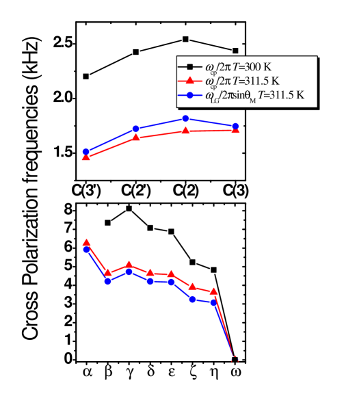
Figure 2.11: Cross-Polarization frequencies obtained from the LG and standard CP experiments for all the non-quaternary carbons in the molecule. Note that the signal corresponding to C($\alpha$) does not appear at $300{}\operatorname{K}$; also note that the signal of C($\beta$) merges with that of C($\delta$) at $311.5\operatorname{K}$ so the same value of frequency has been assigned to both carbons.

this relation is not satisfied for aromatic carbons. Considering that C($\gamma$) is exactly on-resonance and that the H-H condition was optimized for that carbon, the disagreement can be attributed to a non negligible mismatch of the Hartmann-Hahn condition for carbons in the aromatic part of the spectrum. Taking into account a mismatch $\Delta$ for the aromatic carbons, the CP frequency for the LG experiment becomes,

$$\omega_{\mathrm{LG}}=\sqrt{2\left(b/\hbar\right)^{2}(\mathop{\rm sen}\nolimits\theta_{\mathrm{m}})^{2}+\Delta^{2}}.$$

In the standard CP experiment, two frequencies appear, where the observable one is

$$\omega=\frac{\omega^{+}+\omega^{-}}{2}$$ (2.126)

with

$$\omega^{\pm}=\sqrt{\frac{\left[\left(d/\hbar\right)\pm 4\Delta\right]^{2}}{16}+2\left(b/\hbar\right)^{2}}.$$

The other modulating frequency is too low to be observed in the presence of relaxation. Although it is difficult to quantify exactly the magnitude of $\Delta$, we can see that the effect of the mismatch is greater for $\omega_{\mathrm{LG}}$ than for $\omega$ where there is a partial compensation between the two contributing frequencies $\omega^{\pm}$. This explains why $\omega_{\mathrm{LG}}\gtrapprox\omega$ for the carbons in the aromatic part, in contrast with eq. (2.125).

For carbons irradiated on-resonance (aliphatic part), the values of the fitted parameters $b$ and $d$ obtained from standard CP experiments can be compared with the parameters obtained from the LG-CP. In the later case, the parameter of interest is $\omega_{\mathrm{LG}}.$ Then, $b$ is obtained in a direct way from expression (2.124) and $d$ can be obtained comparing $\omega_{\mathrm{LG}}$ with the corresponding value of $\omega$ at the same temperature. Using both experiments, $d$ is calculated from

$$\frac{d}{\hbar}=\frac{4}{\kappa}\sqrt{\omega^{2}-\frac{\omega_{\mathrm{LG}}^{2}}{(\mathop{\rm sen}\nolimits\theta_{\mathrm{m}})^{2}}}.$$ (2.127)

The values of $d$ calculated in this way with $\kappa=1$ (aliphatic carbons) can be compared with those obtained by fitting eq. (2.119) to the standard CP data, i.e. coming from a single experiment.

Table 2.2 displays the values of the homonuclear and heteronuclear couplings for the aliphatic carbons obtained from the standard CP experiment, and combining this with the LG-CP performed at the same temperature. Fig 2.12 allows for the comparison of the ¹³C-¹H and ¹H-¹H couplings obtained from the two methods. As expected, an excellent agreement can be observed for the values of $b$. The novel methodology to estimate $d$ values seems to yield good results within an error of around $20\%$, which could be easily improved by taking longer time data. However, there are no many experimental estimations of these homonuclear couplings and those obtained directly from the ¹H spectra are in good agreement with the values obtained here.

Figure 2.12: Effective homonuclear $\left(1/2\pi\right)\left(d/\hbar\right)$ and heteronuclear $\left(1/2\pi\right)\left(b/\hbar\right)$ dipolar couplings for carbons in the alkyl chain, obtained from the LG and standard CP experiments performed at $311.5{}\operatorname{K}$ (nematic mesophase).

With regard to the relaxation of the system in the CP experiments, we can observe an anisotropic behavior for both phases, quantified by the ratios $\Gamma_{\mathrm{ZZ}}/\Gamma_{\mathrm{XY}}>1$ (see fig. 2.13). Besides, we note that there is an important difference between the behaviors of the nematic and smectic phases. In the nematic phase, the anisotropy can be explained with a purely dipolar model. The average anisotropy factor for all the carbons in the molecule is $(4\pm 1).$ In contrast, in the smectic phase the factor $\Gamma_{\mathrm{ZZ}}/\Gamma_{\mathrm{XY}}>4$ reveals a highly anisotropic behavior for most of the carbons. This can be appreciated in fig. 2.10, where the amplitude of the first maximum is higher than the following ones, specially for the aliphatic carbons. This fact is not observed in nematics, giving support to the purely dipolar anisotropy. Different factors can produce this high anisotropy, one could be $H_{1}$ inhomogeneity, another could be that our main system is actually larger than $SI_{2}$. Although both factors would effectively increase the anisotropy, the effect should be comparable in both phases. Moreover, under the same $H_{1}$ inhomogeneity, we have not observed such anisotropy ratios in molecular crystals. Alternatively, the large anisotropy observed in the smectic phase can be originated on the lack of fast fluctuations in this more rigid phase, which would prevent the application of the extreme narrowing approximation. If we release this approximation and assume that the spectral densities $\mathcal{J}(0)$ and $\mathcal{J}(\Sigma/2)$, although different between them, are approximately constant in an interval of width $2\omega_{0}$, our calculations indicate that $\Gamma_{\mathrm{ZZ}}$ is proportional to $\mathcal{J}(0)$, while $\Gamma_{\mathrm{XY}}\propto\mathcal{J}(\Sigma/2).$ As usually $\mathcal{J}(0)>\mathcal{J}(\Sigma/2),$ this could explain the higher anisotropy in the smectic phase, where motion is more hindered than in the nematic phase.

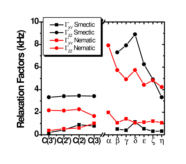
Figure 2.13: Relaxation factors $\Gamma_{\mathrm{ZZ}}$ and $\Gamma_{\mathrm{XY}}$ obtained by fitting the standard CP data to the anisotropic model [eq. (2.119)].

2.3 Summary

We solved the spin dynamics of many-spin systems. First, we started solving the dynamics of a two-spin system interacting with a fast fluctuating spin-bath. We extended [ÁLP07] the solution of MKBE [MKBE74] starting from the system-environment Hamiltonian to obtain the relaxation superoperator. We solved the spin dynamics for an anisotropic SE interaction [ÁLP07], where the anisotropy is given by the ratio between the Ising and XY contributions. Müller, et al. used a phenomenological isotropic relaxation for the SE interaction. Here, we emphasize the different sources of the anisotropy in the decoherence and relaxation processes. The main difference is that while the XY interaction takes the systems to the total system equilibrium, the Ising SE interaction takes it to an internal quasi-equilibrium [CÁL⁺03, ÁLP07]. In the particular case of an isotropic SE interaction, we reproduce the MKBE solution. These solutions were obtained neglecting the non-secular terms of the SE interaction with respect to the system Hamiltonian, i.e. under the condition $b\gg\Gamma_{\mathrm{SE}}.$ We extended the solution including the non-secular terms [ÁLP07] as will be fully discussed in chapter 3.

In section § 2.2, we further extended the MKBE model to solve the spin dynamics of a three-spin system interacting with a fast fluctuating spin-bath [CÁL⁺03]. Our calculations were performed for three-spin configurations directly applicable to the $8$CB molecule. This molecule has two possible configurations for the heteronuclear couplings that led us to realize that in each space of $M=\pm 1/2$ there are only two of the three eigenstates involved in the dipolar transitions that give rise to the oscillations. This is a consequence of the symmetry of the system, i.e. the flip-flop can only occur between the carbon and one combination of the proton states (the symmetric or the antisymmetric) depending on the relative signs of the heteronuclear couplings ($b_{1}=b_{2}$ or $b_{1}=-b_{2}$) [CÁL⁺03]. We showed that this affects the oscillation frequency that one measures experimentally.

In section § 2.2.3, we introduced ¹³C-¹H cross-polarization experiments which complemented with the detailed spin dynamics calculations allowed us to obtain separately the homonuclear and heteronuclear dipolar couplings in CH₂ systems [CÁL⁺03]. The reliability of the obtained values was tested with a direct determination of the heteronuclear couplings using CP under Lee-Goldburg conditions. Comparing the standard CP experiments with the LG-CP one, we concluded that the last one is better to determine directly the ¹³C-¹H couplings. However, the standard CP allows one to obtain homonuclear couplings in addition to the heteronuclear couplings. This experiment is also important to get further information of the system as for example the relaxation phenomena.

From the theoretical analysis of the CH₂ dynamics, we recognized two different time scales for the decoherence behavior given by $\Gamma_{\mathrm{ZZ}}$ and $\Gamma_{\mathrm{XY}}.$ Besides, the CP data showed that the rate of attenuation of the oscillations is much faster than the rate of polarization transfer from the bath. This anisotropy could be explained in the nematic phase by assuming a dipolar interaction Hamiltonian between the three-spin system and the bath within the extreme narrowing approximation. In the smectic phase, however, the anisotropy is much more pronounced and it seems that the short time fluctuations of the bath approximation is not appropriate. Consideration of a slow motion regime leads to a better agreement with the experimental observations without resorting to other mechanisms which operate in both phases [CÁL⁺03].

Chapter 3 Spin dynamics within another perspective: The Keldysh formalism

As we discuss in previous chapters, the characterization and control of spin dynamics in open and close spin systems of intermediate size remains a problem of great interest [MLL03]. However, the quantum interferences of these systems become damped by the lack of isolation from the environment and one visualizes this phenomenon as decoherence. Indeed, the inclusion of the degrees of freedom of the environment may easily become an unsolvable problem and requires approximations not fully quantified. This motivates a revival of interest on previous studies in various fields such as Nuclear Magnetic Resonance [MKBE74], quantum transport [DP90] and the quantum-classical correspondence problem [PZ99, Zur03] with a view on their application to emergent fields like the quantum computation [WL02, DRKH03, TSS⁺00] and molecular electronics [MKR94, PGIN03, LY01, Zim03].

The most standard framework adopted to describe the system-environment interaction is the one that we used in the previous chapter, the generalized Liouville-von Neumann equation [Abr61, EBW91] in the fast fluctuation approximation. There, the degrees of freedom of the environment are traced out to yield a quantum master equation (QME), eq. (2.39). Interactions with the environment occur at a rate given by the Fermi Golden Rule (FGR) providing a dissipative mechanism that could induce a non unitary dynamics into the system. An overall (conservation) balance condition is obtained by imposing a convergence into the thermal equilibrium state (2.49). While sufficient for the most traditional applications, this approximation leaves aside important memory effects and interferences in the time domain produced by the coherent interaction between the system and the bath [TIL03].

A less known alternative is provided by the Keldysh formalism [Kel64] in the integral representation proposed by Danielewicz [Dan84]. On one side, it uses the well known perturbation to infinite order in selected terms provided by the Feynman diagrams where, under certain conditions that go beyond the Fermi Golden Rule, the dynamical feedback effects become relevant. On the other, this integral representation has the advantage of being able to profit from a Wigner representation for the time-energy domain. This last representation is particularly meaningful in the fermionic case since it allows one to define energy states and their occupations simultaneously with the physical time [Pas92]. In that case, one can transform the Danielewicz equation into the generalized Landauer-Büttiker equation (GLBE) [Pas91, Pas92] to solve the quantum dynamics of the system. The Keldysh formalism already inspired original experimental and theoretical developments in coherent spin dynamics involving quantum interferences in the time domain. In particular, it was used to develop the notion of polarization waves leading to mesoscopic echoes [PLU95, PUL96], to establish the influence of chaos on time reversal (Loschmidt echoes) [LUP98, PLU⁺00, JP01] and to propose a spin projection chromatography [DPL04]. A rough account of many-body decoherence enabled the interpretation of anomalies in “spin diffusion” experiments as a manifestation of the quantum Zeno effect [PU98]. This technique was applied to a case with an exact analytical solution [DPL02] and where more standard approximations can be obtained to show the potential of our proposal. Our model represents a single fermion that can jump between two states while an external fermionic reservoir is coupled to one of them. This environment provides decoherence due to a through space Coulomb interaction and can feed the system with an extra particle through tunneling processes. While the parameters and approximations involved in this model are especially designed to be mapped to a problem of spin dynamics (the two-spin system of chapter 2), it could also be adapted to represent a double quantum dot charge qubit [VMB05]. In that case, a double dot is operated in the gate voltage regime where there is a single electron which can jump between the two coupled states. Only one of these states is coupled to an electron reservoir. We introduce fictitious interactions to obtain a common interaction rate which leads to a homogeneous non-hermitian effective Hamiltonian. In the specific model considered, we analyze how different SE interactions, e.g. tunneling to the leads and through space Coulomb interaction, modify the quantum evolution. A particular advantage of the fictitious symmetrization is that it leads naturally to a stroboscopic representation of the SE processes. This leads to a very efficient numerical algorithm where the quantum dynamics is obtained in a sequence of time steps. Finally, we resort to the Jordan-Wigner mapping between fermions and spins to apply the procedure to a spin system. This allows us to give a first-principle derivation of the self-energies to explain, in chapter 4, the puzzling experimental dynamics observed in a spin swapping gate [LUP98] (see fig. 1.6).

3.1 Two level system dynamics

3.1.1 The system

Consider a two fermion state system interacting with the following Hamiltonian $\widehat{\mathcal{H}}_{\mathrm{S}}$,

$$\widehat{\mathcal{H}}_{\mathrm{S}}=E_{0}\hat{c}_{0}^{+}\hat{c}_{0}+E_{1}\hat{c}_{1}^{+}\hat{c}_{1}-V_{01}\left(\hat{c}_{0}^{+}\hat{c}_{1}+\hat{c}_{1}^{+}\hat{c}_{0}\right),$$ (3.1)

with $\hat{c}_{i}^{+}(\hat{c}_{i})$ the standard fermionic creation (destruction) operators. The $E_{i}$ are the energies of the $i$-th local states whose spin index is omitted and $V_{12}$ the hopping interaction. In matrix representation, if we have only one particle in the system, we have a $2\times 2$ matrix for the Hamiltonian

$$\begin{array}[c]{ccc}&\begin{array}[c]{cc}\left|1,0\right\rangle&\left|0,1\right\rangle\end{array}&\\ \mathcal{H}_{\mathrm{S}}=&\left(\begin{array}[c]{cc}E_{0}&-V_{01}\\ -V_{01}&E_{1}\end{array}\right)&\begin{array}[c]{c}\left|1,0\right\rangle\\ \left|0,1\right\rangle\end{array}.\end{array}$$ (3.2)

Here $\left|1,0\right\rangle$ and $\left|0,1\right\rangle$ denote the states with the particle in the level $0$ and $1$ respectively.

3.1.2 System evolution

We are interested in the study of the evolution of an initial local excitation in the system. For definiteness, we consider the initial excitation on site $1$ which is described by the non-equilibrium state $\left|\Psi\left(0\right)\right\rangle=\hat{c}_{1}^{+}\left|0,0\right\rangle=\left|0,1\right\rangle$ where $\left|0,0\right\rangle$ is the vacuum state. The probability to find the particle in the state $0$ and $1$ is

$$P_{01}\left(t\right) =\left|\left\langle 1,0\right|\Psi\left(t\right)\right|^{2},$$ (3.3)

$$P_{11}\left(t\right) =\left|\left\langle 0,1\right|\Psi\left(t\right)\right|^{2},$$ (3.4)

where

$$\left|\Psi\left(t\right)\right\rangle=\exp\left\{-\mathrm{i}\widehat{\mathcal{H}}_{\mathrm{S}}~{}t\right\}\left|\Psi\left(0\right)\right\rangle.$$ (3.5)

Thus, we obtain if $E_{0}=E_{1}$

$$P_{01}\left(t\right) =\frac{1}{2}-\frac{1}{2}\cos\left(\omega_{0}t\right),$$ (3.6)

$$P_{11}\left(t\right) =\frac{1}{2}+\frac{1}{2}\cos\left(\omega_{0}t\right),$$ (3.7)

where $\omega_{0}=2V_{01}/\hbar$ gives the natural oscillation frequency of the transition between the states $0$ and $1$. The fig. 3.1

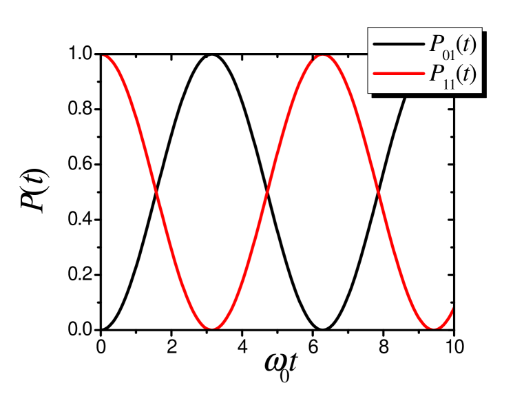
Figure 3.1: Evolution of the probabilities to find a particle in site $0$ (black line) and site $1$ (red line) with the initial conditions at site $1.$

show the dynamics of these probabilities.

3.2 A two level system interacting with a particle reservoir

3.2.1 The system

Let’s consider the electron two-state system of the previous section asymmetrically coupled to an electron reservoir, as shown in fig. 3.2 a),

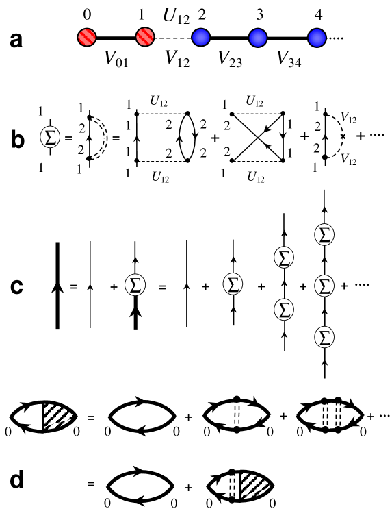
Figure 3.2: a) System-environment (SE) representation. Dashed circles and solid circles represent the system and the environment states respectively. Dashed lines are hopping interactions while wiggels lines are through-space Coulomb interactions. b) Self-enegy diagram summing up the different interactions with the environment in a local basis. The lines with arrows are exact Green’s functions in absence of SE interactions. The double dashed line represents the effective SE interaction. c) Retarded Green’s function at site $0$. The interaction with the environment is to infinite order in the self-energy given in b) . d) Particle density function at site $0$. The double dashed lines represent the effective interactions local in time and space summed up to infinity order.

with the total Hamiltonian

$$\widehat{\mathcal{H}}=\widehat{\mathcal{H}}_{\mathrm{S}}+\widehat{\mathcal{H}}_{\mathrm{E}}+\widehat{\mathcal{H}}_{\mathrm{SE}}.$$ (3.8)

The system Hamiltonian is the same described in the previous section (3.1)

$$\widehat{\mathcal{H}}_{\mathrm{S}}=E_{0}\hat{c}_{0}^{+}\hat{c}_{0}+E_{1}\hat{c}_{1}^{+}\hat{c}_{1}-V_{01}\left(\hat{c}_{0}^{+}\hat{c}_{1}+\hat{c}_{1}^{+}\hat{c}_{0}\right),$$ (3.9)

with $\hat{c}_{i}^{+}(\hat{c}_{i})$ the standard fermionic creation (destruction) operators. The hopping interaction $V_{01}$ gives the natural frequency, $\omega_{0}=2V_{01}/\hbar$, of the transition between the states $0$ and $1$. The environment has a similar Hamiltonian,

$$\widehat{\mathcal{H}}_{\mathrm{E}}=\sum_{i=2}^{\infty}E_{i}\hat{c}_{i}^{+}\hat{c}_{i}-\sum_{\genfrac{}{}{0.0pt}{}{i=2}{j>i}}^{\infty}V_{ij}\left(\hat{c}_{i}^{+}\hat{c}_{j}+\hat{c}_{j}^{+}\hat{c}_{i}\right),$$ (3.10)

where the $V_{ij}$ determines the topology of the interaction network in the environment states. The system-environment (SE) interaction is described by

$$\widehat{\mathcal{H}}_{\mathrm{SE}}=\sum_{\alpha,\beta=\uparrow,\downarrow}\left[U_{12}^{(\mathrm{dir.})}~{}\hat{c}_{1,\beta}^{+}\hat{c}_{1,\beta}\hat{c}_{2,\alpha}^{+}\hat{c}_{2,\alpha}+U_{12}^{(\mathrm{exch.})}~{}\hat{c}_{1,\alpha}^{+}\hat{c}_{2,\alpha}\hat{c}_{2,\alpha}^{+}\hat{c}_{1,\alpha}-V_{12}\left(\hat{c}_{1,\alpha}^{+}\hat{c}_{2,\alpha}+\hat{c}_{2,\alpha}^{+}\hat{c}_{1,\alpha}\right)\right],$$ (3.11)

The first two terms on the rhs represent the Coulomb interaction of an electron in site $1$ with an electron in site $2,$ the first site of the reservoir. $U_{12}^{(\mathrm{dir.})}$ is the standard direct integral and $U_{12}^{(\mathrm{exch.})}$ is the small exchange integral which we include for completeness The third term is the hopping interaction between sites $1$ and $2$.

3.2.2 System evolution

3.2.2.1 Quantum dynamics within the Keldysh formalism

Now, we have a many-body system and we consider it in the thermodynamical many-body equilibrium state $\left|\Psi_{\mathrm{eq.}}\right\rangle$. In the infinity temperature limit, it has all the states equally occupied. We are interested in the study of the evolution of an initial local excitation in the system. Thus, as we consider previously for definiteness, let’s consider the initial excitation with a particle on site $1$ and a hole in site $0$ which is described by the non-equilibrium state

$$\left|\Psi_{\mathrm{n.e.}}\right\rangle=\hat{c}_{1}^{+}\hat{c}_{0}\left|\Psi_{\mathrm{eq.}}\right\rangle.$$ (3.12)

The evolution in a complete norm preserving solution is described by the particle and hole density functions,

$$G_{ij}^{<}\left(t_{2},t_{1}\right)=\frac{\mathrm{i}}{\hbar}\left\langle\Psi_{\mathrm{n.e.}}\right|\hat{c}_{j}^{+}\left(t_{1}\right)\hat{c}_{i}\left(t_{2}\right)\left|\Psi_{\mathrm{n.e.}}\right\rangle$$ (3.13)

and

$$G_{ij}^{>}\left(t_{2},t_{1}\right)=-\frac{\mathrm{i}}{\hbar}\left\langle\Psi_{\mathrm{n.e.}}\right|\hat{c}_{i}\left(t_{2}\right)\hat{c}_{j}^{+}\left(t_{1}\right)\left|\Psi_{\mathrm{n.e.}}\right\rangle,$$ (3.14)

that describe spatial and temporal correlations. In these expressions, the creation and destruction operators are in the Heisenberg representation. Notice that, in contrast with the equilibrium definitions of $G_{ij}^{\lessgtr\,}(t_{2},t_{1}),$ now they have an implicit dependence on the initial local excitation. The probability amplitude of finding a particle in site $i$ at time $t_{2}$ when initially was in site $j$ at time $t_{1}$ is described by the retarded Green’s function of the whole system

$$G_{ij}^{\mathrm{R}}\left(t_{2},t_{1}\right) =\theta\left(t_{2},t_{1}\right)\ [G_{ij}^{>}\left(t_{2},t_{1}\right)-G_{ij}^{<}\left(t_{2},t_{1}\right)]$$

$$=\left[G_{ji}^{\mathrm{A}}\left(t_{1},t_{2}\right)\right]^{\ast}.$$ (3.15)

The reduced density function $\mathbf{G}^{<}\left(t,t\right)$, where matrix indices are restricted to $i,j\in\left\{0,1\right\}$, is equivalent to the single particle $2\times 2$ density matrix and $\mathbf{G}^{\mathrm{R}}\left(t_{2},t_{1}\right)$ is an effective evolution operator. If the system is isolated, the Green’s function in its energy representation is obtained by a Fourier transform (FT) respect to the time interval $\delta t=t_{2}-t_{1}$

$$\mathbf{G}^{0\mathrm{R}}\left(\varepsilon,t\right)=\int\mathbf{G}^{0\mathrm{R}}\left(t+\tfrac{1}{2}\delta t,t-\tfrac{1}{2}\delta t\right)\exp[\mathrm{i}\varepsilon\delta t/\hbar]\mathrm{d}\delta t,$$ (3.16)

where $t=\frac{1}{2}\left(t_{2}+t_{1}\right).$ In a time independent system:

$$\mathbf{G}^{0\mathrm{R}}\left(\varepsilon,t\right)\equiv\mathbf{G}^{0\mathrm{R}}\left(\varepsilon\right)=[\varepsilon\mathbf{I}-\mathbf{H}_{\mathrm{S}}]^{-1}.$$ (3.17)

After including SE interactions, the Green’s function defines the reduced effective Hamiltonian and the self-energy $\mathbf{\Sigma}^{\mathrm{R}}(\varepsilon)$ [LPD90],

$$\mathbf{H}_{\mathrm{eff.}}(\varepsilon)\equiv\varepsilon\mathbf{I}-\left[\mathbf{G}^{\mathrm{R}}\left(\varepsilon\right)\right]^{-1}=\mathbf{H}_{\mathrm{S}}+\mathbf{\Sigma}^{\mathrm{R}}(\varepsilon).$$ (3.18)

Here, the exact perturbed dynamics is contained in the nonlinear dependence of the self-energy $\mathbf{\Sigma}^{\mathrm{R}}$ on $\varepsilon$. For infinite reservoirs the evolution with $\mathbf{H}_{\mathrm{eff.}}$ is non-unitary, hence, the Green’s function has poles at the “eigenenergies”, $\varepsilon_{\nu}$, that have imaginary components [DP90],

$$-2\operatorname{Im}\Sigma^{\mathrm{R}}\left(\varepsilon_{\nu}\right)/\hbar=1/\tau_{\mathrm{SE}}=2\Gamma_{\mathrm{SE}}/\hbar.$$ (3.19)

These account for the “decay rates” into collective SE eigenstates in agreement with a self-consistent Fermi Golden Rule (FGR) [FP06]. Similarly, $\operatorname{Re}\Sigma^{\mathrm{R}}\left(\varepsilon_{\nu}\right)=\operatorname{Re}\varepsilon_{\nu}-\varepsilon_{\nu}^{0}$ represent the “shifts” of the system’s eigenenergies $\varepsilon_{\nu}^{0}.$

The evolution of the density function for the reduced open system is described using the Keldysh formalism [Kel64, Dan84]. The density function in the Danielewicz form [Dan84] is

$$\mathbf{G}^{<}\left(t_{2},t_{1}\right)=\hbar^{2}\mathbf{G}^{\mathrm{R}}\left(t_{2},0\right)\mathbf{G}^{<}\left(0,0\right)\mathbf{G}^{\mathrm{A}}\left(0,t_{1}\right)\\ +\int_{0}^{t_{2}}\int_{0}^{t_{1}}\mathrm{d}t_{k}\mathrm{d}t_{l}\mathbf{G}^{\mathrm{R}}\left(t_{2},t_{k}\right)\mathbf{\Sigma}^{<}\left(t_{k},t_{l}\right)\mathbf{G}^{\mathrm{A}}\left(t_{l},t_{1}\right).$$ (3.20)

The first term is the “coherent” evolution while the second term contains “incoherent reinjections” through the self-energy function, $\mathbf{\Sigma}^{<}$. This compensates any leak from the coherent evolution reflected by the imaginary part of $\Sigma^{\mathrm{R}}$ (see [Pas92]). The key to solve eq. (3.20) is to build up an expression for the particle (hole) injection and retarded self-energies, $\mathbf{\Sigma}^{<(>)}\left(t_{1},t_{2}\right)$ and

$$\mathbf{\Sigma}^{\mathrm{R}}\left(t_{1},t_{2}\right)=\theta\left(t_{1},t_{2}\right)[\mathbf{\Sigma}^{>}\left(t_{2},t_{1}\right)-\mathbf{\Sigma}^{<}\left(t_{2},t_{1}\right)].$$ (3.21)

For this purpose, we use a perturbative expansion on $\widehat{\mathcal{H}}_{\mathrm{SE}}$ for the Coulomb interaction [DÁLP07] and the hopping interaction [DPÁ05]. The first order in the perturbation expansion is the standard Hartree-Fock energy correction which does not contribute to $\Sigma^{<}$ because it is real. We focus on the second order terms, with Feynman diagrams sketched in fig. 3.2 b).

The injection self energy is

$$\Sigma_{ij}^{\lessgtr}\left(t_{k},t_{l}\right)=\left|U_{12}\right|^{2}\hbar^{2}G_{22}^{\lessgtr}\left(t_{k},t_{l}\right)G_{22}^{\gtrless}\left(t_{l},t_{k}\right)G_{11}^{\lessgtr}\left(t_{k},t_{l}\right)~{}\delta_{i1}\delta_{1j}+\left|V_{12}\right|^{2}G_{22}^{\lessgtr}\left(t_{k},t_{l}\right)~{}\delta_{i1}\delta_{1j},$$ (3.22)

where $U_{12}=-2U_{12}^{(\mathrm{dir.})}+U_{12}^{(\mathrm{exch.})}$ is the net Coulomb interaction between an electron in the system and one in the reservoir. The direct term contributes with a fermion loop and an extra spin summation which is represented in the $-2$ factor [Dan84]. The first term in eq. (3.22) corresponds to the direct and exchange self-energy diagrams shown in the last line of fig. 3.2 b). The first two diagrams schematize the creation of an electron-hole pair in the environment and its later destruction. The last term in eq. (3.22) and the last diagram of the same figure is the hopping to site $2$ which allows the electron to perform a full exploration inside the reservoir. To take into account the different time scales for the dynamics of excitations in the system and in the reservoir, we use the time-energy variables [Pas92]: the physical time $t_{\mathrm{i}}=\frac{1}{2}\left(t_{k}+t_{l}\right),$and the domain of quantum correlations $\delta t_{\mathrm{i}}=t_{k}-t_{l}.$ This last is related to an energy $\varepsilon$ through a FT [Pas92]. Thus, in equilibrium,

$$G_{22}^{<}\left(\varepsilon,t_{\mathrm{i}}\right) =\mathrm{i}2\pi~{}N_{2}\left(\varepsilon\right)~{}\mathrm{f}_{2}\left(\varepsilon,t_{\mathrm{i}}\right),$$ (3.23)

$$G_{22}^{>}\left(\varepsilon,t_{\mathrm{i}}\right) =-\mathrm{i}2\pi~{}N_{2}\left(\varepsilon\right)~{}\left[1-\mathrm{f}_{2}\left(\varepsilon,t_{\mathrm{i}}\right)\right],$$ (3.24)

where $N_{2}\left(\varepsilon\right)$ is the local density of states (LDoS) at the surface of the reservoir. Assuming that the environment stays in the thermodynamical equilibrium and $k_{\mathrm{B}}T$ is much higher that any energy scale in the bath (high temperature limit), the occupation factor is

$$\mathrm{f}_{2}\left(\varepsilon,t_{\mathrm{i}}\right)=\mathrm{f}_{2}.$$ (3.25)

Fourier transforming on $\varepsilon$ one obtains

$$G_{22}^{<}\left(t_{\mathrm{i}}+\tfrac{\delta t_{\mathrm{i}}}{2},t_{\mathrm{i}}-\tfrac{\delta t_{\mathrm{i}}}{2}\right)=\mathrm{i}2\pi\mathrm{~{}}g_{2}\left(\delta t_{\mathrm{i}}\right)~{}\mathrm{f}_{2}$$ (3.26)

and

$$G_{22}^{>}\left(t_{\mathrm{i}}+\tfrac{\delta t_{\mathrm{i}}}{2},t_{\mathrm{i}}-\tfrac{\delta t_{\mathrm{i}}}{2}\right)=-\mathrm{i}2\pi\mathrm{~{}}g_{2}\left(\delta t_{\mathrm{i}}\right)~{}\left(1-\mathrm{f}_{2}\right),$$ (3.27)

where

$$g_{2}\left(\delta t_{\mathrm{i}}\right)=\int N_{2}\left(\varepsilon\right)e^{-\mathrm{i}\varepsilon\delta t_{\mathrm{i}}}\frac{\mathrm{d}\varepsilon}{2\pi\hbar}.$$ (3.28)

Replacing in eq. (3.22)

$$\Sigma_{ij}^{\lessgtr}\left(t_{\mathrm{i}}+\tfrac{\delta t_{\mathrm{i}}}{2},t_{\mathrm{i}}-\tfrac{\delta t_{\mathrm{i}}}{2}\right)=\left|U_{12}\right|^{2}\hbar^{2}\left(2\pi\right)^{2}\left[g_{2}\left(\delta t_{\mathrm{i}}\right)\right]^{2}\mathrm{f}_{2}\left[1-\mathrm{f}_{2}\right]G_{11}^{\lessgtr}\left(t_{\mathrm{i}}+\tfrac{\delta t_{\mathrm{i}}}{2},t_{\mathrm{i}}-\tfrac{\delta t_{\mathrm{i}}}{2}\right)\delta_{i1}\delta_{1j}\\ \pm\left|V_{12}\right|^{2}~{}\mathrm{i}2\pi g_{2}\left(\delta t_{\mathrm{i}}\right)~{}\left(\genfrac{}{}{0.0pt}{}{\mathrm{f}_{2}}{1-\mathrm{f}_{2}}\right)~{}\delta_{i1}\delta_{1j},$$ (3.29)

where the $\left(\genfrac{}{}{0.0pt}{}{\mathrm{f}_{2}}{1-\mathrm{f}_{2}}\right)$ associates $\mathrm{f}_{2}$ with $\Sigma^{<}$ and $\left(1-\mathrm{f}_{2}\right)$ with $\Sigma^{>}$.

In summary, we are left with the task to evaluate the time dependent self energies and the integral in eq. (3.20). We will focus in the parametric regime corresponding to the experimental conditions of the spin swapping gate (cross-polarization) described in section § 2.1.2.

3.2.2.2 An environment in the wide band or fast fluctuation regime

As occurs with the generalized Landauer-Büttiker equations for linear transport, an essential ingredient is the possibility to assign a Markovian nature to the environment. We are going to see that this appears naturally from the formalism when the dynamics of excitations within the environment is faster than the time scales relevant to the system. In order to separate the different physical time scales involved in the problem, we start changing to the time-energy variables in eq. (3.20). Evaluating in $t_{2}=t_{1}=t,$ the integrand becomes

$$\int_{0}^{t}\mathrm{d}t_{\mathrm{i}}\int_{-t}^{t}\mathrm{d}\delta t_{\mathrm{i}}\mathbf{G}^{\mathrm{R}}\left(t,t_{\mathrm{i}}+\tfrac{\delta t_{\mathrm{i}}}{2}\right)\mathbf{\Sigma}^{<}\left(t_{\mathrm{i}}+\tfrac{\delta t_{\mathrm{i}}}{2},t_{\mathrm{i}}-\tfrac{\delta t_{\mathrm{i}}}{2}\right)\mathbf{G}^{\mathrm{A}}\left(t_{\mathrm{i}}-\tfrac{\delta t_{\mathrm{i}}}{2},t\right).$$ (3.30)

The environment unperturbed Green’s function $g_{2}\left(\delta t_{\mathrm{i}}\right)$ decays within the time scale $\hbar/V_{\mathrm{B}}$ where $V_{\mathrm{B}}$ is the characteristic interaction inside the reservoir. In the wide band regime ($V_{\mathrm{B}}\gg V_{01}$) $\hbar/V_{\mathrm{B}}$ becomes much shorter than the characteristic evolution time of $G_{11}^{\lessgtr}\left(t_{\mathrm{i}}+\tfrac{\delta t_{\mathrm{i}}}{2},t_{\mathrm{i}}-\tfrac{\delta t_{\mathrm{i}}}{2}\right)$ given by $\hbar/V_{01}.$ Then, as the main contribution to the integral on $\delta t_{\mathrm{i}}$ of eq. (3.20) is around the time scale $\hbar/V_{\mathrm{B}}$ we can replace $G_{11}^{\lessgtr}\left(t_{\mathrm{i}}+\tfrac{\delta t_{\mathrm{i}}}{2},t_{\mathrm{i}}-\tfrac{\delta t_{\mathrm{i}}}{2}\right)$ by $G_{11}^{\lessgtr}\left(t_{\mathrm{i}},t_{\mathrm{i}}\right)$. Following the same assumption we replace $G^{\mathrm{R}}\left(t,t_{\mathrm{i}}+\frac{\delta t_{\mathrm{i}}}{2}\right)$ by $G^{\mathrm{R}}\left(t,t_{\mathrm{i}}\right)$ and $G^{\mathrm{A}}\left(t_{\mathrm{i}}-\frac{\delta t_{\mathrm{i}}}{2},t\right)$ by $G^{\mathrm{A}}\left(t_{\mathrm{i}},t\right).$ In this fast fluctuation regime, only $\Sigma_{ij}^{\lessgtr}\left(t_{\mathrm{i}}+\tfrac{\delta t_{\mathrm{i}}}{2},t_{\mathrm{i}}-\tfrac{\delta t_{\mathrm{i}}}{2}\right)$ depends on $\delta t_{\mathrm{i}}$ leading to

$$\Sigma_{ij}^{\lessgtr}\left(t_{\mathrm{i}}\right)=\int_{-t}^{t}\Sigma_{ij}^{\lessgtr}\left(t_{\mathrm{i}}+\tfrac{\delta t_{\mathrm{i}}}{2},t_{\mathrm{i}}-\tfrac{\delta t_{\mathrm{i}}}{2}\right)\mathrm{d}\delta t_{\mathrm{i}}\\ =\left|U_{12}\right|^{2}\hbar^{2}\left(2\pi\right)^{2}\left[\int_{-t}^{t}\left[g_{2}\left(\delta t_{\mathrm{i}}\right)\right]^{2}\mathrm{d}\delta t_{\mathrm{i}}\right]\mathrm{f}_{2}\left[1-\mathrm{f}_{2}\right]G_{11}^{\lessgtr}\left(t_{\mathrm{i}},t_{\mathrm{i}}\right)~{}\delta_{i1}\delta_{1j}\\ \pm\left|V_{12}\right|^{2}~{}\mathrm{i}2\pi\left[\int_{-t}^{t}g_{2}\left(\delta t_{\mathrm{i}}\right)\mathrm{d}\delta t_{\mathrm{i}}\right]\left(\genfrac{}{}{0.0pt}{}{\mathrm{f}_{2}}{1-\mathrm{f}_{2}}\right)\delta_{i1}\delta_{1j},$$ (3.31)

which is local in space and time. This assumption for the time scales can be seen in fig. 3.2 b) as a collapse of a pair of black dots, along a vertical line, into a single point. This justifies the expansion of fig. 3.2 c) and the use of the ladder approximation containing only vertical interaction lines in fig. 3.2 d).

Assuming $E_{i}=0$ for $i=1,..,\infty$ we obtain for the decay rates

$$\frac{1}{\tau_{\mathrm{SE}}} \equiv\tfrac{\mathrm{i}}{\hbar}\left(\Sigma_{11}^{\mathrm{A}}-\Sigma_{11}^{\mathrm{R}}\right)$$

$$=\tfrac{\mathrm{i}}{\hbar}\left(\Sigma_{11}^{>}-\Sigma_{11}^{<}\right)$$

$$=\left|U_{12}\right|^{2}~{}\left(2\pi\right)^{2}\left[\int_{-t}^{t}\left[g_{2}\left(\delta t_{\mathrm{i}}\right)\right]^{2}\mathrm{d}\delta t_{\mathrm{i}}\right]~{}\mathrm{f}_{2}\left[1-\mathrm{f}_{2}\right]+\tfrac{1}{\hbar}\left|V_{12}\right|^{2}~{}2\pi\left[\int_{-t}^{t}g_{2}\left(\delta t_{\mathrm{i}}\right)\mathrm{d}\delta t_{\mathrm{i}}\right]$$

$$=\tfrac{2}{\hbar}\left(\Gamma_{U}+\Gamma_{V}\right),$$ (3.32)

where we have used $t\gg\hbar/V_{\mathrm{B}}$ to define

$$\Gamma_{U}=\hbar\left|U_{12}\right|^{2}~{}2\pi^{2}\left[\int_{-\infty}^{\infty}\left[g_{2}\left(\delta t_{\mathrm{i}}\right)\right]^{2}\mathrm{d}\delta t_{\mathrm{i}}\right]~{}\mathrm{f}_{2}\left[1-\mathrm{f}_{2}\right],$$ (3.33)

the Coulomb decay rate, and

$$\Gamma_{V}=\left|V_{12}\right|^{2}~{}\pi\left[\int_{-\infty}^{\infty}g_{2}\left(\delta t_{\mathrm{i}}\right)\mathrm{d}\delta t_{\mathrm{i}}\right],$$ (3.34)

the hopping decay rate. If one assumes that the environment (3.10) can be represented by a linear chain with all the hoppings equal to $V_{\mathrm{B}}$ the LDoS is [DPÁ05]:

$$N_{2}\left(\varepsilon\right)=1/\left(\pi V_{\mathrm{B}}\right)\sqrt{1-\left(\frac{\varepsilon}{2V_{\mathrm{B}}}\right)^{2}}.$$ (3.35)

Thus, the Green’s function

$$g_{2}\left(\delta t_{\mathrm{i}}\right)=\frac{1}{2\pi V_{\mathrm{B}}}\frac{J_{1}\left(\frac{2V_{\mathrm{B}}}{\hbar}\delta t_{i}\right)}{\delta t_{i}}$$ (3.36)

is proportional to the first order Bessel function and decays within a characteristic time $\hbar/V_{\mathrm{B}}.$ Assuming that $\mathrm{f}_{2}=1/2$ and the integration limits in the $\Gamma$’s expressions are taken to infinity because $t\sim\hbar/V_{01}\gg\hbar/V_{\mathrm{B}}$ (wide band approximation), one obtains

$$\Gamma_{U}=\tfrac{2\pi}{\hbar}\left|U_{12}\right|^{2}\dfrac{2}{3\pi^{2}V_{\mathrm{B}}}$$ (3.37)

and

$$\Gamma_{V}=\tfrac{2\pi}{\hbar}\left|V_{12}\right|^{2}\frac{1}{\pi V_{\mathrm{B}}}.$$ (3.38)

It is important to remark that the wide band limit can be relaxed because the FGR holds when time $t$ is in the range [FP06] $t_{\mathrm{B}}<t<t_{\mathrm{R}}\simeq\alpha\hbar/\Gamma_{\mathrm{SE}}\ln(V_{\mathrm{B}}/\Gamma_{\mathrm{SE}}),$ where $\alpha$ depends on the van Hove singularities of the spectral density $\mathcal{J}_{\mathrm{2}}(\varepsilon)=\int N_{\mathrm{2}}(\varepsilon-\varepsilon^{\prime})N_{\mathrm{2}}(\varepsilon^{\prime})\mathrm{d}\varepsilon^{\prime}$. Here, $t_{\mathrm{B}}=\hbar\mathcal{J}_{\mathrm{2}}(0)\simeq\hbar/V_{\mathrm{B}}$ is the survival time of an electron-hole excitation at the surface site and $t_{\mathrm{R}}$ characterizes the transition to a power law decay arising from memory effects. Hence, as long as $\Gamma_{\mathrm{SE}},V_{01}\ll V_{\mathrm{B}},$ the FGR is valid for times much longer than $\hbar/\Gamma_{\mathrm{SE}}$.

Since the interaction is local in time, the reduced density results:

$$\mathbf{G}^{<}\left(t,t\right)=\hbar^{2}\mathbf{G}^{\mathrm{R}}\left(t,0\right)\mathbf{G}^{<}\left(0,0\right)\mathbf{G}^{\mathrm{A}}\left(0,t\right)+\int_{0}^{t}\mathrm{d}t_{\mathrm{i}}\mathbf{G}^{\mathrm{R}}\left(t,t_{\mathrm{i}}\right)\mathbf{\Sigma}^{<}\left(t_{\mathrm{i}}\right)\mathbf{G}^{\mathrm{A}}\left(t_{\mathrm{i}},t\right),$$ (3.39)

which is complemented with

$$\mathbf{\Sigma}^{<}\left(t_{\mathrm{i}}\right)=\left(\begin{array}[c]{cc}0&0\\ 0&2\Gamma_{U}\hbar G_{11}^{<}\left(t_{\mathrm{i}},t_{\mathrm{i}}\right)+2\Gamma_{V}\hbar\left(\frac{\mathrm{i}}{\hbar}\mathrm{f}_{2}\right)\end{array}\right).$$ (3.40)

Here, the propagators $\mathbf{G}^{\mathrm{R}}\left(t,0\right)$ and $\mathbf{G}^{\mathrm{A}}\left(0,t\right)$ that enter in both terms are obtained from the effective Hamiltonian of the reduced system,

$$\mathbf{H}_{\mathrm{eff.}}=\left(\begin{array}[c]{cc}0&-V_{01}\\ -V_{01}&-\mathrm{i}\Gamma_{\mathrm{SE}}\end{array}\right),$$ (3.41)

where $\Gamma_{\mathrm{SE}}$ is energy independent. This results in an equation of the form of the GLBE. However, the Hamiltonian is asymmetric in the SE interaction complicating the form of the associated propagator. The apparent complexity to solve this equation contrasts with the homogeneous case where the evolution of the GLBE was obtained [Pas91] through a Laplace transform. Our strategy will be to induce such form of symmetry.

3.2.2.3 A fictitious homogeneous decay

The main difficulty with the eq. (3.39) is that it involves multiple exponentials. In order to create propagators with an homogeneous decay, i.e. a single exponential factor, we introduce fictitious interactions, $\mathbf{\Sigma}_{\mathrm{fic.}}^{\mathrm{R}},~{}$with the environment. The symmetric Hamiltonian becomes

$$\mathbf{H}_{\mathrm{sym.}} =\mathbf{H}_{\mathrm{eff.}}+\mathbf{\Sigma}_{\mathrm{fic.}}^{\mathrm{R}}$$

$$=\left(\begin{array}[c]{cc}0&-V_{01}\\ -V_{01}&-\mathrm{i}\Gamma_{\mathrm{SE}}\end{array}\right)+\left(\begin{array}[c]{cc}-\mathrm{i}\frac{1}{2}\Gamma_{\mathrm{SE}}&0\\ 0&\mathrm{i}\frac{1}{2}\Gamma_{\mathrm{SE}}\end{array}\right)$$ (3.46)

$$=\left(\begin{array}[c]{cc}-\mathrm{i}\frac{1}{2}\Gamma_{\mathrm{SE}}&-V_{12}\\ -V_{12}&-\mathrm{i}\frac{1}{2}\Gamma_{\mathrm{SE}}\end{array}\right).$$ (3.49)

Here $\mathbf{\Sigma}_{\mathrm{fic.}}^{\mathrm{R}}$ includes the fictitious interactions which, in the present case, produce a leak of probability in site $0$ at a rate $\Gamma_{\mathrm{SE}}/\hbar$ while in site $1$ inject probability at the same rate. Both states of $\mathbf{H}_{\mathrm{sym.}}$ interact with the environment independently with the same characteristic rate $\Gamma_{\mathrm{SE}}/\hbar.$ Note that this rate is half the real value. The propagators of eq. (3.20) have now a simple dependence on $t$ as

$$\mathbf{G}^{\mathrm{R}}\left(t,0\right)=\mathbf{G}^{0\mathrm{R}}\left(t,0\right)e^{-\frac{\Gamma_{\mathrm{SE}}}{2}t/\hbar},$$ (3.50)

where

$$G_{00}^{0\mathrm{R}}(t,0)=G_{11}^{0\mathrm{R}}(t,0)=\frac{\mathrm{i}}{\hbar}\cos\left(\frac{\omega_{0}}{2}t\right)$$ (3.51)

and

$$G_{01}^{0\mathrm{R}}(t,0)=G_{10}^{0\mathrm{R}}(t,0)^{\ast}=\frac{\mathrm{i}}{\hbar}\mathop{\rm sen}\nolimits\left(\frac{\omega_{0}}{2}t\right)$$ (3.52)

are the isolated system propagators. The reduced density evolution is now,

$$\mathbf{G}^{<}\left(t,t\right)=\hbar^{2}\mathbf{G}^{0\mathrm{R}}\left(t,0\right)\mathbf{G}^{<}\left(0,0\right)\mathbf{G}^{0\mathrm{A}}\left(0,t\right)e^{-t/2\tau_{\mathrm{SE}}}\\ +\int_{0}^{t}\mathrm{d}t_{\mathrm{i}}\mathbf{G}^{0\mathrm{R}}\left(t,t_{\mathrm{i}}\right)\mathbf{\Sigma}_{\mathrm{sym.}}^{<}\left(t_{\mathrm{i}}\right)\mathbf{G}^{0\mathrm{A}}\left(t_{\mathrm{i}},t\right)e^{-\left(t-t_{\mathrm{i}}\right)/2\tau_{\mathrm{SE}}},$$ (3.53)

which is similar to the GLBE [Pas91, Pas92]. It is easy to see that the introduction of negative/positive imaginary parts in the diagonal energies of the effective Hamiltonian produces a decay/growth rates of the elements of the density function which, being fictitious, must be compensated by a fictitious injection self-energy

$$\Sigma_{\mathrm{fic.},ij}^{<}\left(t_{\mathrm{i}}\right)=-\hbar\operatorname{Im}\left(\Sigma_{\mathrm{fic.},ii}^{\mathrm{R}}+\Sigma_{\mathrm{fic.},jj}^{\mathrm{R}}\right)G_{ij}^{<}\left(t_{\mathrm{i}},t_{\mathrm{i}}\right).$$ (3.54)

In our case, this results in an injection that includes the compensation effects for the symmetrized interaction,

$$\mathbf{\Sigma}_{\mathrm{sym.}}^{<}\left(t_{\mathrm{i}}\right)=\mathbf{\Sigma}^{<}\left(t_{\mathrm{i}}\right)+\mathbf{\Sigma}_{\mathrm{fic.}}^{<}\left(t_{\mathrm{i}}\right)\\ =\left(\begin{array}[c]{cc}0&0\\ 0&2\Gamma_{U}\hbar G_{11}^{<}\left(t_{\mathrm{i}},t_{\mathrm{i}}\right)+2\Gamma_{V}\hbar\left(\frac{\mathrm{i}}{\hbar}\mathrm{f}_{2}\right)\end{array}\right)+\left(\begin{array}[c]{cc}\Gamma_{\mathrm{SE}}\hbar G_{00}^{<}\left(t_{\mathrm{i}},t_{\mathrm{i}}\right)&0\\ 0&-\Gamma_{\mathrm{SE}}\hbar G_{11}^{<}\left(t_{\mathrm{i}},t_{\mathrm{i}}\right)\end{array}\right).$$ (3.55)

Here, the second term is proportional to the local density functions $G_{ii}^{<}\left(t_{\mathrm{i}},t_{\mathrm{i}}\right)$ injecting and extracting density on sites $0$ and $1$ respectively to restore the real occupation. We can rewrite the last expression to separate the processes that involve density relaxation (through injection and escape processes) and pure decoherence (through local energy fluctuations):

$$\mathbf{\Sigma}_{\mathrm{sym.}}^{<}\left(t_{\mathrm{i}}\right) =\Sigma_{\mathrm{i}}^{<}\left(t_{\mathrm{i}}\right)+\Sigma_{\mathrm{m}}^{<}\left(t_{\mathrm{i}}\right)$$

$$=\mathrm{i}\Gamma_{\mathrm{SE}}\left[2p_{V}\left(\begin{array}[c]{cc}0&0\\ 0&\left(\mathrm{f}_{2}-\frac{\hbar}{\mathrm{i}}G_{11}^{<}\left(t_{\mathrm{i}},t_{\mathrm{i}}\right)\right)\end{array}\right)+\left(\begin{array}[c]{cc}\frac{\hbar}{\mathrm{i}}G_{00}^{<}\left(t_{\mathrm{i}},t_{\mathrm{i}}\right)&0\\ 0&\frac{\hbar}{\mathrm{i}}G_{11}^{<}\left(t_{\mathrm{i}},t_{\mathrm{i}}\right)\end{array}\right)\right].$$ (3.60)

Here

$$\frac{\hbar}{\mathrm{i}}G_{11}^{<}\left(t_{\mathrm{i}},t_{\mathrm{i}}\right)\equiv\frac{\hbar}{\mathrm{i}}\int G_{11}^{<}\left(\varepsilon,t_{\mathrm{i}}\right)\frac{\mathrm{d}\varepsilon}{2\pi\hbar}=\mathrm{f}_{1}\left(t_{\mathrm{i}}\right)$$ (3.61)

and

$$\frac{\hbar}{\mathrm{i}}G_{00}^{<}\left(t_{\mathrm{i}},t_{\mathrm{i}}\right)=\mathrm{f}_{0}\left(t_{\mathrm{i}}\right),$$ (3.62)

while

$$p_{V}=\Gamma_{V}/\Gamma_{\mathrm{SE}}$$ (3.63)

is the weight of the tunneling rate relative to the total SE interaction rate. As the initial state has the site $2$ occupied we have that

$$\frac{\hbar}{\mathrm{i}}G_{ij}^{<}\left(0,0\right)=\delta_{i1}\delta_{1j}.$$ (3.64)

Introducing eq. (3.60) into eq. (3.53) and using

$$\frac{1}{\tau_{\mathrm{SE}}}\equiv\tfrac{2}{\hbar}\Gamma_{\mathrm{SE}}$$ (3.65)

we get two coupled equations for $G_{00}^{<}$ and $G_{11}^{<}$

$$\tfrac{\hbar}{\mathrm{i}}G_{00}^{<}\left(t,t\right)=\left|\hbar G_{01}^{0\mathrm{R}}\left(t,0\right)\right|^{2}e^{-t/\left(2\tau_{\mathrm{SE}}\right)}+\\ \int\left|\hbar G_{01}^{0\mathrm{R}}\left(t,t_{\mathrm{i}}\right)\right|^{2}e^{-\left(t-t_{\mathrm{i}}\right)/2\tau_{\mathrm{SE}}}~{}2p_{V}~{}\frac{\mathrm{d}t_{\mathrm{i}}}{2\tau_{\mathrm{SE}}}\left[\mathrm{f}_{2}-\tfrac{\hbar}{\mathrm{i}}G_{11}^{<}\left(t_{\mathrm{i}},t_{\mathrm{i}}\right)\right]\\ +\int\left|\hbar G_{00}^{0\mathrm{R}}\left(t,t_{\mathrm{i}}\right)\right|^{2}e^{-(t-t_{\mathrm{i}})/\left(2\tau_{\mathrm{SE}}\right)}\frac{\mathrm{d}t_{\mathrm{i}}}{2\tau_{\mathrm{SE}}}\left[\tfrac{\hbar}{\mathrm{i}}G_{00}^{<}\left(t_{\mathrm{i}},t_{\mathrm{i}}\right)\right]\\ +\int\left|\hbar G_{01}^{0\mathrm{R}}\left(t,t_{\mathrm{i}}\right)\right|^{2}e^{-(t-t_{\mathrm{i}})/\left(2\tau_{\mathrm{SE}}\right)}\frac{\mathrm{d}t_{\mathrm{i}}}{2\tau_{\mathrm{SE}}}\left[\tfrac{\hbar}{\mathrm{i}}G_{11}^{<}\left(t_{\mathrm{i}},t_{\mathrm{i}}\right)\right].$$ (3.66)

$$\tfrac{\hbar}{\mathrm{i}}G_{11}^{<}\left(t,t\right)=\left|\hbar G_{11}^{0\mathrm{R}}\left(t,0\right)\right|^{2}e^{-t/\left(2\tau_{\mathrm{SE}}\right)}+\\ \int\left|\hbar G_{11}^{0\mathrm{R}}\left(t,t_{\mathrm{i}}\right)\right|^{2}e^{-\left(t-t_{\mathrm{i}}\right)/2\tau_{\mathrm{SE}}}~{}2p_{V}~{}\frac{\mathrm{d}t_{\mathrm{i}}}{2\tau_{\mathrm{SE}}}\left[\mathrm{f}_{2}-\tfrac{\hbar}{\mathrm{i}}G_{11}^{<}\left(t_{\mathrm{i}},t_{\mathrm{i}}\,\right)\right]\\ +\int\left|\hbar G_{10}^{0\mathrm{R}}\left(t,t_{\mathrm{i}}\right)\right|^{2}e^{-(t-t_{\mathrm{i}})/\left(2\tau_{\mathrm{SE}}\right)}\frac{\mathrm{d}t_{\mathrm{i}}}{2\tau_{\mathrm{SE}}}\left[\tfrac{\hbar}{\mathrm{i}}G_{00}^{<}\left(t_{\mathrm{i}},t_{\mathrm{i}}\right)\right]\\ +\int\left|\hbar G_{11}^{0\mathrm{R}}\left(t,t_{\mathrm{i}}\right)\right|^{2}e^{-(t-t_{\mathrm{i}})/\left(2\tau_{\mathrm{SE}}\right)}\frac{\mathrm{d}t_{\mathrm{i}}}{2\tau_{\mathrm{SE}}}\left[\tfrac{\hbar}{\mathrm{i}}G_{11}^{<}\left(t_{\mathrm{i}},t_{\mathrm{i}}\right)\right].$$ (3.67)

In each equation, the first term is the probability that a particle initially at site $1$ be found in site $0$ (or $1$) at time $t$ having survived the interactions with the environment with a probability $e^{-t/\left(2\tau_{\mathrm{SE}}\right)}$. The second term describes the process of injection/escape of particles enabled by the hopping from/towards the reservoir, where the last of such processes occurred in the time range ($t_{\mathrm{i}},t_{\mathrm{i}}+\mathrm{d}t_{i}$) with a probability $2p_{V}\frac{\mathrm{d}t_{\mathrm{i}}}{2\tau_{\mathrm{SE}}}.$ The injection/escape is produced on site $1$ and fill/empty the site to level it to the occupation factor $\mathrm{f}_{2}$. The third and fourth terms take into account the last process of measurement at time $t_{\mathrm{i}}$ due to the SE interaction with a probability $\tfrac{\mathrm{d}t_{\mathrm{i}}}{2\tau_{\mathrm{SE}}}$. This confirms our interpretation that in eq. (3.60) the dissipation processes are in $\mathbf{\Sigma}_{\mathrm{i}}^{<}\left(t\right)$ while $\mathbf{\Sigma}_{\mathrm{m}}^{<}\left(t\right)$ involves pure decoherence. It is clear that by iterating this formula, one gets a series in the form represented in fig. 3.2 d).

3.2.2.4 The dynamics of a swapping gate

The solution of the coupled eqs. (3.66) and (3.67) involves a Laplace transform. We consider a parameter range compatible with the spin problem where $\mathrm{f}_{2}\lesssim 1$ while we allow the tunneling relative weight $p_{V}$ in the range $\left[0,1\right]$.  In a compact notation, the density function results:

$$P_{01}\left(t\right)=\tfrac{\hbar}{\mathrm{i}}G_{00}^{<}\left(t,t\right)=1-a_{0}e^{-R_{0}t}-a_{1}\cos\left[\left(\omega+\mathrm{i}\eta\right)t+\varphi_{0}\right]e^{-R_{1}t}.$$ (3.68)

Here, the decay rates $R_{0},~{}R_{1}$ and $\eta$, and the oscillation frequency $\omega$ are real numbers associated with poles of the Laplace transform. The amplitude $a_{0}$ is also real while, when $\omega=0,$ the amplitude $a_{1}$ and the initial phase $\varphi_{0}$ acquire an imaginary component that warrants a real density. These observables have expressions in terms of adimensional functions of the fundamental parameters in the model. Denoting

$$x=\omega_{0}\tau_{\mathrm{SE}}$$ (3.69)

and remembering that

$$p_{V}=\Gamma_{V}/\Gamma_{\mathrm{SE}},$$ (3.70)

we define

$$\phi\left(p_{V},x\right)=\frac{1}{3}\left(x^{2}-p_{V}^{2}-\frac{1}{3}\left(1-p_{V}\right)^{2}\right),$$ (3.71)

and

$$\chi\left(p_{V},x\right)=\left\{4\left(1-p_{V}\right)\left(9x^{2}-2\left(1-p_{V}\right)^{2}+18p_{V}^{2}\right)\right.\\ \left.+12\left[3\left(4x^{6}-\left(\left(1-p_{V}\right)^{2}+12p_{V}^{2}\right)x^{4}\right.\right.\right.\\ \left.\left.\left.+4p_{V}^{2}\left(5\left(1-p_{V}\right)^{2}+3p_{V}^{2}\right)x^{2}-4p_{V}^{2}\left(\left(1-p_{V}\right)^{2}-p_{V}^{2}\right)^{2}\right)\right]^{\frac{1}{2}}\right\}^{\frac{1}{3}}.$$ (3.72)

The observable “frequency”,

$$\omega+\mathrm{i}\eta=\frac{\sqrt{3}}{2x}\left(\frac{1}{6}\chi\left(p_{V},x\right)+6\frac{\phi\left(p_{V},x\right)}{\chi\left(p_{V},x\right)}\right)\omega_{0},$$ (3.73)

is purely real or imaginary, i.e. $\omega\eta\equiv 0$. Also,

$$R_{0} =\left(6\frac{\phi\left(p_{V},x\right)}{\chi\left(p_{V},x\right)}-\frac{1}{6}\chi\left(p_{V},x\right)+p_{V}+\frac{1}{3}\left(1-p_{V}\right)\right)\frac{1}{\tau_{\mathrm{SE}}},$$ (3.74)

$$R_{1} =\frac{3}{2}\left(p_{V}+\frac{1}{3}\left(1-p_{V}\right)\right)\frac{1}{\tau_{\mathrm{SE}}}-\frac{R_{0}}{2},$$ (3.75)

and

$$a_{0} =\frac{1}{2}\frac{2\left(\omega^{2}-\eta^{2}\right)+2R_{1}^{2}-\omega_{0}^{2}}{\left(\omega^{2}-\eta^{2}\right)+\left(R_{0}-R_{1}\right)^{2}},$$ (3.76)

$$a_{2} =\dfrac{1}{2\left(\omega+\mathrm{i}\eta\right)}\frac{\left(2R_{0}R_{1}-\omega_{0}^{2}\right)\left(R_{0}-R_{1}\right)+2\left(\omega^{2}-\eta^{2}\right)R_{0}}{\left(\omega^{2}-\eta^{2}\right)+\left(R_{0}-R_{1}\right)^{2}},$$ (3.77)

$$a_{3} =\frac{1}{2}\frac{\omega_{0}^{2}+2R_{0}^{2}-4R_{0}R_{1}}{\left(\omega^{2}-\eta^{2}\right)+\left(R_{0}-R_{1}\right)^{2}},$$ (3.78)

$$a_{1}^{2} =a_{2}^{2}+a_{3}^{2},\;\;\;\;\;\tan\left(\phi_{0}\right)=-\frac{a_{2}}{a_{3}}.$$ (3.79)

The oscillation frequency $\omega$ in eq. (3.73) has a critical point $x_{\mathrm{c}}$ at a finite value of $x$ showing, as we called, a quantum dynamical phase transition [ÁDLP06, DÁLP07] for which $\omega$ and $\eta$ in eq. (3.68) exchange their roles as being zero and having a finite value respectively. A full discussion of this issue for a spin system will be presented in chapter 4. Here, the dynamical behavior changes from a swapping phase to an overdamped phase. This last regime can be associated with the Quantum Zeno effect [MS77] where frequent projective measurements prevent the quantum evolution. Here, this is a dynamical effect [PU98, PN94] produced by interactions with the environment that freeze the system oscillation.

Fig. 3.3 shows typical curves of $\tfrac{\hbar}{\mathrm{i}}G_{00}^{<}\left(t,t\right)$ in the swapping phase. The different colors correspond to different SE interactions rates, $p_{V}=0$, $0.5$ and $1,$ which are Coulomb $\left(\Gamma_{V}=0\right)$, isotropic $\left(\Gamma_{V}=\Gamma_{U}\right)$ and pure tunneling $\left(\Gamma_{U}=0\right)$ interactions rates. The hopping interaction does not conserve the net energy in the system inducing a dissipation which is manifested through the non conservation of the number of particles in the system. This is the case of $p_{V}\neq 0$ where the final state of the system has the occupation probability of the sites equilibrated with the bath occupation (f₂). In fig. 3.3, this is manifested as the asymptotic normalized density (occupation probability) of $1$. However, if $p_{V}=0,$ tunneling is forbidden and the system goes to an internal quasi-equilibrium as we described in the eq. (2.63), i.e. the local excitation is spread inside the system. In this case the asymptotic occupation probability of site $0$ is $1/2.$

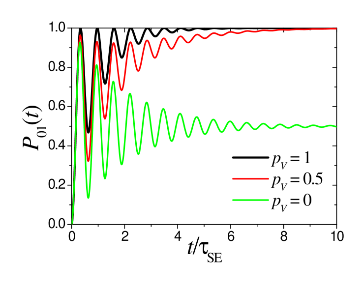
Figure 3.3: Occupation probability, $P_{01}\left(t\right)=$i$G_{00}^{<}\left(t\right)/\hbar,$ to find a particle at site $0$ when initially was at site $1.$ Each line corresponds to different kinds, $p_{V},$ of SE interactions. The plots correspond to $x=V_{01}\tau_{\mathrm{SE}}/\hbar=10$ belonging to the swapping phase and f${}_{2}=1$.

3.3 Stroboscopic process

Eq. (3.39) has two main difficulties for a numerical implementation: The first is the evaluation of the system non-unitary propagators under inhomogeneous perturbations. The second is to keep track of all previous states of the system to enable the integration over previous times. We will show that the decay homogenization enables the implementation of an efficient numerical algorithm. First of all, we identify in expression (3.53) that $e^{-t/\left(2\tau_{\mathrm{SE}}\right)}=s\left(t\right)$ is the system’s survival probability to the environment interruption, i.e., the probability that the system remains coherent, and $\mathrm{d}t_{\mathrm{i}}/(2\tau_{\mathrm{SE}})=q\left(t_{\mathrm{i}}\right)\mathrm{d}t_{\mathrm{i}}$ is the “interruption” probability in a differential time around $t_{\mathrm{i}}$. The interaction of the environment is discretized in intervals $\tau_{\mathrm{str.}}$ where it acts instantaneously. This stroboscopic interaction leads to:

$$s\left(t\right) =\left(1-p\right)^{n\left(t\right)},$$ (3.80)

$$q\left(t\right) =\sum_{m=1}^{\infty}p~{}\delta\left(t-m\tau_{\mathrm{str.}}\right)$$ (3.81)

where

$$n\left(t\right)=\mathrm{int}\left(t/\tau_{\mathrm{str.}}\right).$$ (3.82)

Here, the stroboscopic interruptions may occur at the discrete times $m\tau_{\mathrm{str.}}$ with a probability $p$. At time $t$ there were $n\left(t\right)$ possible interruptions. In the joint limit $\tau_{\mathrm{str.}}\rightarrow 0$ and $p\rightarrow 0$ such that

$$p/\tau_{\mathrm{str.}}=1/\left(2\tau_{\mathrm{SE}}\right),$$ (3.83)

we can recover the continuous expression. To do this, notice that if $n\left(t\right)=n,$ one can write eq. (3.80) as

$$s\left(t\right)=\left(1-p\right)^{\frac{\left(n\tau_{\mathrm{str.}}\right)}{\tau_{\mathrm{str.}}}}=\left(1-\frac{\tau_{\mathrm{str.}}}{2\tau_{\mathrm{SE}}}\right)^{\left(n\tau_{\mathrm{str.}}\right)/\tau_{\mathrm{str.}}}.$$ (3.84)

If $t=n\tau_{\mathrm{str.}}$ then

$$s\left(t\right)=\left(1-\frac{\tau_{\mathrm{str.}}}{2\tau_{\mathrm{SE}}}\right)^{t/\tau_{\mathrm{str.}}}.$$ (3.85)

By taking the limit $\tau_{\mathrm{str.}}\rightarrow 0$ the variable $t$ becomes continuous yielding

$$s\left(t\right) =\lim_{\tau_{\mathrm{str.}}\rightarrow 0}\left(1-\frac{\tau_{\mathrm{str.}}}{2\tau_{\mathrm{SE}}}\right)^{t/\tau_{\mathrm{str.}}}$$

$$=\exp\left[-t/\left(2\tau_{\mathrm{SE}}\right)\right],$$ (3.86)

which is the continuous expression for $s\left(t\right).$

Then, by substituting $p=\tau_{\mathrm{str.}}/(2\tau_{\mathrm{SE}})$ in eq. (3.81) we have

$$q(t)=\frac{1}{2\tau_{\mathrm{SE}}}\sum_{m=1}^{\infty}\tau_{\mathrm{str.}}\delta(t-m\tau_{\mathrm{str.}}).$$ (3.87)

In the limit $\tau_{\mathrm{str.}}\rightarrow 0,$ $t_{m}=m\tau_{\mathrm{str.}}$ becomes a continuous variable and we can convert the sum into an integral, leading to continuous expression of the GLBE (3.53):

$$q(t)=\frac{1}{2\tau_{\mathrm{SE}}}\int_{0}^{\infty}\tau_{\mathrm{str.}}\delta(t-t_{m})\frac{\mathrm{d}t_{m}}{\tau_{\mathrm{str.}}}=\frac{1}{2\tau_{\mathrm{SE}}}.$$ (3.88)

Coming back to the discrete version, we introduce eqs. (3.80) and (3.81) into the reduced density expression (3.53) to obtain

$$\mathbf{G}^{<}\left(t,t\right)=\hbar^{2}\mathbf{G}^{0\mathrm{R}}\left(t,0\right)\mathbf{G}^{<}\left(0,0\right)\mathbf{G}^{0\mathrm{A}}\left(0,t\right)\left(1-p\right)^{n(t)}\\ +\int_{0}^{t}\mathrm{d}t_{\mathrm{i}}\tau_{\mathrm{SE}}\sum_{m=1}^{\infty}\delta\left(t_{\mathrm{i}}-t_{m}\right)\mathbf{G}^{0\mathrm{R}}\left(t,t_{\mathrm{i}}\right)\mathbf{\Sigma}_{\mathrm{sym.}}^{<}\left(t_{\mathrm{i}}\right)\mathbf{G}^{0\mathrm{A}}\left(t_{\mathrm{i}},t\right)p\left(1-p\right)^{n(t-t_{\mathrm{i}})}.$$ (3.89)

After integration, we obtain

$$\mathbf{G}^{<}\left(t,t\right)=\hbar^{2}\mathbf{G}^{0\mathrm{R}}\left(t,0\right)\mathbf{G}^{<}\left(0,0\right)\mathbf{G}^{0\mathrm{A}}\left(0,t\right)\left(1-p\right)^{n}\\ +\hbar^{2}\sum_{m=1}^{n}\mathbf{G}^{0\mathrm{R}}\left(t,t_{m}\right)\delta\mathbf{G}_{\mathrm{inj.}}^{<}\left(t_{m},t_{m}\right)\mathbf{G}^{0\mathrm{A}}\left(t,t_{m}\right)p\left(1-p\right)^{n-m},$$ (3.90)

where $n=n(t),$ $t_{m}=m\tau_{\mathrm{str.}}$ and

$$\delta\mathbf{G}_{\mathrm{inj.}}^{<}\left(t,t\right)=\frac{2\tau_{\mathrm{SE}}}{\hbar^{2}}\mathbf{\Sigma}_{\mathrm{sym.}}^{<}\left(t\right).$$ (3.91)

In this picture, the evolution between interruptions is governed by the system’s propagators

$$\mathbf{G}^{0\mathrm{R}}\left(t,0\right)=-\frac{\mathrm{i}}{\hbar}\exp[-\mathrm{i}\mathbf{H}_{\mathrm{S}}t/\hbar]$$ (3.92)

and

$$\mathbf{G}^{0\mathrm{A}}\left(0,t\right)=\mathbf{G}^{0\mathrm{R}}\left(t,0\right)^{{\dagger}}.$$ (3.93)

The spin-bath stroboscopically interrupts the system evolution producing the decay of the coherent beam. This decay is compensated through the reinjection of probability (or eventually of coherences) expressed in the instantaneous interruption function, $\delta\mathbf{G}_{\mathrm{inj.}}^{<}\left(t,t\right)$, which also contains actual injection/decay from/to the bath.

The first term in the rhs of eq. (3.90) is the coherent system evolution weighted by its survival probability $\left(1-p\right)^{n}.$ This is the upper branch in fig. 3.4. The second term is the incoherent evolution involving all the decoherent branches. The $m$-th term in the sum represents the evolution that had its last interruption at $m\tau_{\mathrm{str.}}$ and since then survived coherently until $n\tau_{\mathrm{str.}}$. Each of these terms is represented in fig. 3.4 by all the branches with an interrupted state (gray dot, red online) at the hierarchy level $m$ after which they survive without further interruptions until $n\tau_{\mathrm{str.}}$. This representation has an immediate resemblance to that introduced by Pascazio and Namiki to justify the dynamical Zeno effect [PN94].

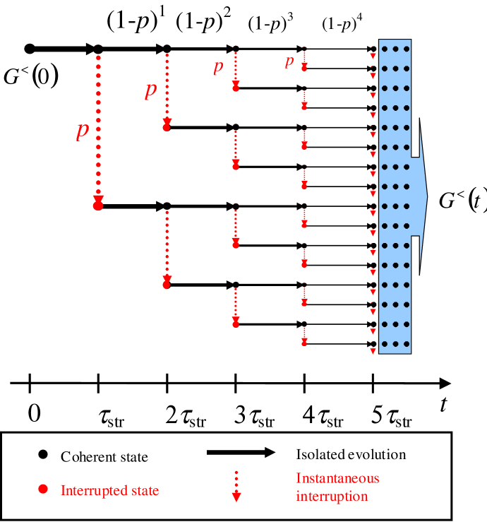
Figure 3.4: Quantum branching sequence for the stroboscopic evolution. Red dots represent states with interrupted (incoherent) evolution while the black dots are coherent with their predecessor. The horizontal continuous arrows represent the isolated evolution and the vertical dashed lines are the instantaneous interruptions. Notice the self-similar structure.

As mentioned above, the solutions of eqs. (3.90) and (3.53) are both computationally demanding since they involve the storage of all the previous steps and reiterated summations. Thus, taking advantage of the self-similarity of the hierarchy levels in the interaction with the environment, we rearrange expression (3.90) into a form optimized for numerical computation,

$$\tfrac{1}{\hbar^{2}}\mathbf{G}^{<}\left(t_{n+1},t_{n+1}\right)=\mathbf{G}^{0\mathrm{R}}\left(t_{n+1},t_{n}\right)\mathbf{G}^{<}\left(t_{n},t_{n}\right)\mathbf{G}^{0\mathrm{A}}\left(t_{n},t_{n+1}\right)\left(1-p\right)\\ +\mathbf{G}^{0\mathrm{R}}\left(t_{n+1},t_{n}\right)\delta\mathbf{G}_{\mathrm{inj.}}^{<}\left(t_{n},t_{n}\right)\mathbf{G}^{0\mathrm{A}}\left(t_{n},t_{n+1}\right)p.$$ (3.94)

This equation provides a new computational procedure that only requires the storage of the density function at a single previous step. Besides, it avoids random averages required in models that include decoherence through stochastic or kicked-like perturbations [TFL⁺03, DCM92].

3.3.1 A nice physical interpretation: The environment as a measurement apparatus

We introduce our computational procedure operationally for an Coulomb interaction form ($V_{12}/U_{12}=0$) of $\widehat{\mathcal{H}}_{\mathrm{SE}}$. The initial state of the isolated two-level system evolves with $\widehat{\mathcal{H}}_{\mathrm{S}}$. At $\tau_{\mathrm{str.}}$, the particle reservoir interacts instantaneously with the “system” interrupting it with a probability $p$. The actual physical time for the SE interaction is then obtained as $\tau_{\mathrm{SE}}=\tau_{\mathrm{str.}}/p$. Considering that the dynamical time scale of the bath ($\tau_{\mathrm{B}}\simeq\hbar/V_{\mathrm{B}}$) is much faster than that of the system (fast fluctuation approximation), the dynamics of site $2$ produces an energy fluctuation on site $1$ that destroys the coherence of the two-level “system”. This represents the “measurement” process that collapses the “system” state. At time $\tau_{\mathrm{str.}}$, the “system” evolution splits into three alternatives: with probability $1-p$ the state survives the interruption and continues its undisturbed evolution, while with probability $p$ the system is effectively interrupted and its evolution starts again from each of the two eigenstates of $\hat{c}_{1}^{+}\hat{c}_{1}$. These three possible states at $\tau_{\mathrm{str.}}$ evolve freely until the system is monitored again at time $2\tau_{\mathrm{str.}}$ and a new branching of alternatives is produced as represented in the scheme of fig. 3.5 a).

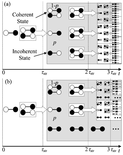
Figure 3.5: Quantum branching sequence for the swapping dynamics. Panel a) stands for a Coulomb system-environment interaction and b) a pure hopping one. Single states represent states with interrupted evolution (incoherent) while pairs of states are coherent superpositions. Notice the self-similar structure.

A similar reasoning holds when $V_{12}\neq 0.$ The sequence for isotropic interaction rates ($\Gamma_{V}=\Gamma_{U}$) is shown in fig. 3.5 b). The hopping part of $\widehat{\mathcal{H}}_{\mathrm{SE}}$ can inject a particle. When an interruption occurs, the bath “measures” at site $2$ and, if found empty, it injects a particle. The inverse process is not considered because we are assuming that the occupation factor in the reservoir is over $1/2$ and we are normalizing the occupation probability to this value. In the figure, this can be interpreted as a “pruning” of some incoherent branches increasing the global coherence. In the next section, we will map the fermion system to a spin system to describe spin dynamics. Thus, this “pruning” explains why the rate of decoherence is greater when the Ising (Coulomb) part of $\widehat{\mathcal{H}}_{\mathrm{SE}}$ dominates over the XY (hopping) part. This occurs with the dipolar interaction and, in less degree, with the isotropic one. This contrasts with a pure XY interaction where the survival of spin coherences is manifested by a “spin wave” behavior.[MBSH⁺97] The empty site of the bath is refilled and de-correlates in a time much shorter than the swapping between sites $0$ and $1$ (fast fluctuation approximation). Consequently, the injection can only occur from the bath toward the system.

3.4 Application to spin systems through the Jordan-Wigner transformation

We apply this procedure to the spin system described in section § 2.1.2 providing a first principle derivation of the phenomenological equations employed there. We consider a system with $M=2$ spins $1/2$ coupled to a spin environment with the following Hamiltonian

$$\widehat{\mathcal{H}}=\widehat{\mathcal{H}}_{\mathrm{S}}+\widehat{\mathcal{H}}_{\mathrm{E}}+\widehat{\mathcal{H}}_{\mathrm{SE}},$$ (3.95)

where the system Hamiltonian, $\widehat{\mathcal{H}}_{\mathrm{S}},$ is described by eq. (2.30)

$$\widehat{\mathcal{H}}_{\mathrm{S}} =\hbar\Omega_{\mathrm{Z}}\left(\hat{S}^{z}+\hat{I}_{1}^{z}\right)+\tfrac{1}{2}b\left(\hat{S}^{+}\hat{I}_{1}^{-}+\hat{S}^{-}\hat{I}_{1}^{+}\right)$$

$$=\hbar\Omega_{\mathrm{Z}}\left(\hat{S}^{z}+\hat{I}_{1}^{z}\right)+b\left(\hat{S}^{x}\hat{I}_{1}^{x}+\hat{S}^{y}\hat{I}_{1}^{y}\right).$$ (3.96)

The environment Hamiltonian is described by

$$\widehat{\mathcal{H}}_{\mathrm{E}}=\sum_{i\geq 2}\hbar\Omega_{\mathrm{Z}}\hat{I}_{i}^{z}+{\textstyle\sum\limits_{\genfrac{}{}{0.0pt}{1}{i\geq 2}{j>i}}}\tfrac{1}{2}b_{ij}\left(\hat{I}_{i}^{+}\hat{I}_{j}^{-}+\hat{I}_{i}^{-}\hat{I}_{j}^{+}\right).$$ (3.97)

This equation, in contrast with eq. (2.32), does not contain the Ising term. Thus, we have here an XY interaction inside the spin-bath instead of the dipolar interaction of section § 2.1.2. The other difference is that the SE interaction described by

$$\widehat{\mathcal{H}}_{\mathrm{SE}}=a_{12}\hat{I}_{1}^{z}\hat{I}_{2}^{z}+\tfrac{1}{2}b_{12}\left(\hat{I}_{1}^{+}\hat{I}_{2}^{-}+\hat{I}_{1}^{-}\hat{I}_{2}^{+}\right),$$ (3.98)

has only one connection between the environment ($\hat{I}_{2}$) and the system ($\hat{I}_{1}$) while the given by eq. (2.31) has many. The purpose of the last simplification is only for a simplified description, but it could be generalized. Remember that, this spin-spin interaction is Ising if $b_{12}/a_{12}=0,$ and $XY$, isotropic (Heisenberg) or the truncated dipolar (secular) if $a_{12}/b_{12}=0,1,-2,$ respectively.

In the previous sections of this chapter we have observed the similarity of the results with the obtained ones in section § 2.1.2. Thus, to use the results obtained within Keldysh formalism we map the spin system into a fermionic system using the Jordan-Wigner Transformation (JWT) [LSM61],

$$\hat{I}_{i}^{+}=\hat{c}_{i}^{+}\exp\left\{\mathrm{i}\pi\sum_{j=1}^{i-1}\hat{c}_{j}^{+}\hat{c}_{j}\right\}.$$ (3.99)

The previous Hamiltonians become

$$\widehat{\mathcal{H}}_{\mathrm{S}} =\hbar\Omega_{\mathrm{Z}}\left(\hat{c}_{0}^{+}\hat{c}_{0}+\hat{c}_{1}^{+}\hat{c}_{1}-\hat{1}\right)+\tfrac{1}{2}b\left(\hat{c}_{0}^{+}\hat{c}_{1}+\hat{c}_{1}^{+}\hat{c}_{0}\right),$$ (3.100)

$$\widehat{\mathcal{H}}_{\mathrm{E}} =\sum_{i\geq 2}\hbar\Omega_{\mathrm{Z}}\left(\hat{c}_{i}^{+}\hat{c}_{i}-\tfrac{1}{2}\hat{1}\right)+{\textstyle\sum\limits_{\genfrac{}{}{0.0pt}{1}{i\geq 2}{j>i}}}\tfrac{1}{2}b_{ij}\left(\hat{c}_{i}^{+}\hat{c}_{j}+\hat{c}_{j}^{+}\hat{c}_{i}\right),$$ (3.101)

$$\widehat{\mathcal{H}}_{\mathrm{SE}} =a_{12}\left(\hat{c}_{1}^{+}\hat{c}_{1}-\tfrac{1}{2}\hat{1}\right)\left(\hat{c}_{2}^{+}\hat{c}_{2}-\tfrac{1}{2}\hat{1}\right)+\tfrac{1}{2}b_{12}\left(\hat{c}_{1}^{+}\hat{c}_{2}+\hat{c}_{2}^{+}\hat{c}_{1}\right),$$ (3.102)

where the index $0$ represents the spin $S.$ Here, the system interacts with the environment through the site $2$ (the surface site of the bath). In the last Hamiltonians, the terms proportional to the identity do not contribute to the dynamics because they only change the total energy by a constant number. This Hamiltonian, as we described in section § 2.1.2, is a standard cross-polarization experiment (swapping gate) in NMR [MKBE74]. In this experiment, the site $S$ is a ¹³C and the site $I_{1}$ a ¹H while the environment is a ¹H spin bath. The typical experimental Hartmann-Hahn condition [HH62] equals the values of the effective energies at the ¹³C and the ¹H sites to optimize the polarization transfer. The SE interaction has terms linear in the number operators $\hat{c}_{1}^{+}\hat{c}_{1}$ and $\hat{c}_{2}^{+}\hat{c}_{2},$ that only change the energy of the sites $1$ and $2$ respectively. Thus, the Hartmann-Hahn implementation, compensates the change of energy produced by the environment through these linear terms. Finally, we have Hamiltonians equivalent to those in eqs. (3.9,3.10,3.11) where the site energies are equal, and $V_{01}=-\frac{b}{2},~{}V_{ij}=-\tfrac{b_{ij}}{2}$, $U_{12}^{\mathrm{(dir.)}}=a_{12}$ and $U_{12}^{\mathrm{(ex.)}}=0.$

The spin dynamics of the system is described by the spin correlation function [DPL04, Dan06]:

$$P_{i1}(t)=\frac{\left\langle\Psi_{\mathrm{eq.}}\right|\hat{I}_{i}^{z}(t)\hat{I}_{1}^{z}(0)\left|\Psi_{\mathrm{eq.}}\right\rangle}{\left\langle\Psi_{\mathrm{eq.}}\right|\hat{I}_{1}^{z}(0)\hat{I}_{1}^{z}(0)\left|\Psi_{\mathrm{eq.}}\right\rangle},$$ (3.103)

which gives the local polarization at time $t$ on the $i$-th spin with an initial local excitation on the $1$-th spin at time $t=0.$ Here, $\left|\Psi_{\mathrm{eq.}}\right\rangle$ is the thermodynamical many-body equilibrium state and

$$\hat{I}_{i}^{z}(t)=e^{\mathrm{i}\widehat{\mathcal{H}}t/\hbar}\hat{I}_{i}^{z}e^{-\mathrm{i}\widehat{\mathcal{H}}t/\hbar}$$ (3.104)

are the spin operators in the Heisenberg representation. After the JWT, the initial local excitation on site $1$ is described by the non-equilibrium state

$$\left|\Psi_{\mathrm{n.e.}}\right\rangle=\hat{c}_{1}^{+}\left|\Psi_{\mathrm{eq.}}\right\rangle.$$ (3.105)

In the experimental high temperature regime, $k_{\mathrm{B}}T$ much larger than any energy scale of the system, the spin correlation function becomes [Dan06]

$$P_{i1}(t)=\tfrac{2\hbar}{\mathrm{i}}G_{ii}^{<\,}(t,t)-1.$$ (3.106)

Notice that $G_{ii}^{<\,}(t,t)$ implicitly depends on the initial local excitation at site $1$. Here, $G_{ii}^{<\,}(t,t)$ is the reduced density function of sites $0$ and $1$ and can be split into the contributions $G_{ii}^{<\,_{(N)}}(t_{2},t_{1})$ from each subspace with $N$ particles (or equivalently $N$ spins up) in the following way,

$$G_{ii}^{<\,}(t,t)=\sum_{N=1}^{M}\dfrac{\left(\genfrac{}{}{0.0pt}{1}{M-1}{N-1}\right)}{2^{M-1}}G_{ii}^{<\,_{(N)}}(t,t),$$ (3.107)

and analogous for the hole density function. The initial condition in this picture is described by

$$G_{ij}^{<_{(N)}}(0,0)=\tfrac{\mathrm{i}}{\hbar}\left(\tfrac{N-1}{M-1}\delta_{ij}+\tfrac{M-N}{M-1}\delta_{i1}\delta_{1j}\right),$$ (3.108)

where the first term is the equilibrium density (identical occupation for all the sites) and the second term is the non-equilibrium contribution where only site $1$ is excited. Thus, we have an expression like (3.20) for each $N$-th subspace [DPÁ05]. For this two-spin system the $-1$ term of eq. (3.106) is canceled out by the background evolution, i.e. the evolution of the first term of eq. (3.108) plus the evolution of the second term of eq. (3.20) for the $N=2$ subspace. As a consequence, the observable dynamics only depends on the initial local excitation at site $1,$

$$G_{ij}^{<_{\left(1\right)}}(0,0)=\tfrac{\mathrm{i}}{\hbar}\delta_{i1}\delta_{1j},$$ (3.109)

and evolves in the $1$-th particle subspace,

$$P_{i1}(t)=\tfrac{\hbar}{\mathrm{i}}G_{ii}^{<\,_{(1)}}(t,t).$$ (3.110)

Finally, the solution of the polarization $P_{01}(t),$ with $\Gamma_{\mathrm{XY}}\leftrightarrow\Gamma_{V}$ and $\Gamma_{\mathrm{ZZ}}\leftrightarrow\Gamma_{U},$ is the same that was obtained in eq. (3.68).

3.4.1 Keldysh formalism versus the generalized quantum master equation

Typical solutions of the quantum master equation for a spin swapping [CÁL⁺03, ÁLP07], described in chapter 2, were obtained following that of Müller et al. [MKBE74]. They considered an isotropic interaction with the spin environment, represented by a phenomenological relaxation rate $R=\Gamma_{\mathrm{XY}}=\Gamma_{\mathrm{ZZ}}=1/\left(4\tau_{\mathrm{SE}}\right).$ Within the fast fluctuation approximation and neglecting non-secular terms, this leads to

$$P^{{}^{\mathrm{MKBE}}}(t)=1-\frac{1}{2}\exp\left[-Rt\right]-\frac{1}{2}\cos(\omega t)\exp\left[-\frac{3}{2}Rt\right],$$ (3.111)

that is obtained from eq. (2.58) in the isotropic case. This expression is used in most of the experimental fittings [PR96, LUP98]. Our eq. (3.68) reproduces this result with $1/\tau_{\phi}\equiv R\simeq 1/\left(4\tau_{\mathrm{SE}}\right)$ by considering an isotropic relation between $\Gamma_{\mathrm{ZZ}}$ and $\Gamma_{\mathrm{XY}},$ i.e. $p_{\mathrm{XY}}=1/2$ under the condition $1/\left(4\tau_{\mathrm{SE}}\right)\ll b/\hbar.$ Note that our microscopic derivation, for an XY chain as environment, does not imply that $\Gamma_{\mathrm{ZZ}}=\Gamma_{\mathrm{XY}}$ comes from an isotropic SE interaction. This conclusion arrives from the expressions (3.37) and (3.38).

Returning to the comparison between expressions (3.111) and (3.68) at short times $t\ll\tau_{\mathrm{SE}},$ one can see that the MKBE swapping probability growths exponentially with a rate $1/\left(4\tau_{\mathrm{SE}}\right)$. In contrast, our solution manifests that the polarization growths quadratically on time, $\left(\frac{1}{2}b/\hbar\right)^{2}t^{2},$ as we anticipated in § 2.1.2.2. In eq. (3.68) this is made possible by the phase $\phi_{0}$ in the cosine. In the parametric region, $b\tau_{\mathrm{SE}}\ll\hbar$,  where MKBE is not valid, our model enables the manifestation of the quantum Zeno effect [MS77, PU98, FP02]. This means that the bath interrupts the system through measurements too frequently, freezing its evolution. Here, this is a dynamical effect [PU98, PN94] produced by interactions with the environment that freezes the system oscillation. At longer times, $t\gg\tau_{\mathrm{SE}}$, one gets

$$1-P_{01}\left(t\right)\sim\left(1+2\left(b/\hbar\right)^{2}\tau_{\mathrm{SE}}^{2}\right)\exp\left[-(b/\hbar)^{2}\tau_{\mathrm{SE}}t\right],$$ (3.112)

and the quantum Zeno effect is manifested in the reduction of the decay rate $1/\tau_{\phi}\propto\left(b/\hbar\right)^{2}\tau_{\mathrm{SE}}$ as $\tau_{\mathrm{SE}}$ gets smaller than $\hbar/b$. This surprising dependence deserves some interpretation. First, we notice that a strong interaction with the bath makes the ¹H spin to fluctuate, according to the Fermi golden rule, at a rate $1/\tau_{\mathrm{SE}}$. The effect on the ¹³C is again estimated in a fast fluctuation approximation as

$$1/\tau_{\phi}\propto\left(b/\hbar\right)^{2}\tau_{\mathrm{SE}}~{}\propto\left(b/\hbar\right)^{2}\left[\left(a_{12}^{2}/\hbar^{2}+b_{12}^{2}/\hbar^{2}\right)\tau_{\mathrm{B}}\right]^{-1}.$$ (3.113)

This “nesting” of two Fermi golden rule rates is formally obtained from a continuous fraction evaluation of the self-energies [LPD90, DPÁ05] involving an infinite order perturbation theory. Another relevant result is that the frequency depends not only on $b$, but also on $\tau_{\mathrm{SE}}$. A remarkable difference between the quantum master equation and our formulation concerns the final state. In the quantum master equation $\sigma_{\infty}$ must be hinted beforehand, while here it is reached dynamically from the interaction with the spin-bath. Here, the reduced density, whose trace gives the system polarization, can fluctuate until it reaches its equilibrium value.

We mentioned in section § 2.1.2.2 that by including the non-secular terms of the SE interaction in the generalized QME, we obtain the expression (3.68) for the polarization evolution. However, here we obtained the solution from a microscopic model using an XY linear chain as the spin environment, without forcing the final state. The Keldysh formalism gives us another perspective to discuss about the physics of quantum evolutions and the interpretation of the approximations made.

It is important to remark that within the fast fluctuation approximation, the temporal and parametric behavior of expression (3.68) does not depend on the environment Hamiltonian. This only appears as an intensity in the values of $\Gamma_{\mathrm{ZZ}}$ and $\Gamma_{\mathrm{XY}}$ and the relation between them (the anisotropy).

3.5 Memory effects of the spin-bath

The ¹³C polarization, $P_{01}(t)$, in the Keldysh formalism arises from the coherent evolution of the initial particle density, for which the environment is a “sink”, and an incoherent contribution where the bath acts as a particle “source”. This can be compared with the complementary framework. Instead of dealing with a “particle” problem we consider it as a “hole” problem [fig. 3.6 b) and c) respectively].

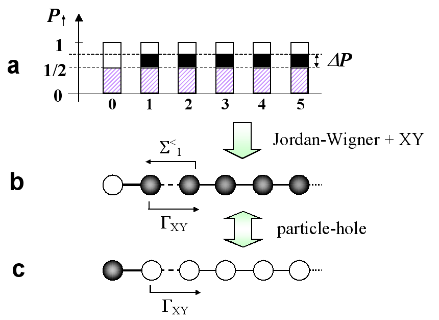
Figure 3.6: a) Schematic representation of the spin system at time $t=0.$ The shaded region stands for the thermodynamic equilibrium state at high temperature and establish a background probability level. The black filling represents the excess of probability over the equilibrium state which is responsible for the observed dynamics. In b) the same system as in a) after the JWT, that is, under the particle point of view. Note that in this situation the background contribution is removed and the dynamics is described by the excess of probability $\Delta P$. In c) we represent the complementary problem of the case b). Here the black filling stands for the hole that represent the excitation. In this representation it is easier to calculate the memory effects in the bath.

On these grounds, at $t=0,$ all the sites are occupied except for the “hole” excitation at the $0$-th site. See fig. 3.6 c) where the black color stands for the hole excitation. At later times this excitation evolves in the system and also propagates through the reservoir. The “environment” does not have holes to inject back into the “system” but those evolved coherently from the initial hole (i.e. $\Sigma^{<}\equiv 0$). Here the environment is a perfect “sink”. Thus all the dynamics would be coherent, in the sense previously explained. If we add the result obtained in this case with that of eq. (3.68) we obtain a one for all times consequence of the particle-hole symmetry. This is a particularly good test of the consistency of the formalism because in each result the “environment” is set in a different framework. It also shows that the background polarization does not contribute to the dynamics as we obtained in (3.110).

This “hole” picture can help us to get a very interesting insight on the dynamics in a case where the memory on the environment becomes relevant. Consider, for example, the case $V_{01}=V_{12}=V_{ij}=V$ and $E_{0}=E_{1}$. The finite version of this effective Hamiltonian applies to the actual experiments reported in ref. [MBSH⁺97]. In this case, the simplifying approximations of the fast fluctuations regime are not justified. However, the exact dynamics of the system can be analytically obtained if one considers an infinite chain. This enables the use of eq. (3.35) to evaluate $\Sigma^{\mathrm{R}}$, eq. (3.21). Then we can calculate the propagator through eq. (3.18) to solve eq. (3.20). The integration gives the first Bessel function, hence:

$$P_{01}(t)=1-\left|\frac{\hbar}{tV}J_{1}(2tV/\hbar)\right|^{2}.$$ (3.114)

A first observation is that the frequency above is roughly increased by a factor of two as compared with that in eq. (3.6). Since the maxima of $P_{01}$ are zeroth of the Bessel function it is clear that the frequency increases slightly with time. These are memory effects of the environment that are dependent on the interplay between the spectral density of the bath and that of the system.

We notice that the memory effect can also appear in other condition for the bath. For example, if the proton nuclei have random polarizations and the density excitation is at site $0$, i.e. in fig. 3.6 a) $\mathrm{f}_{n}(\varepsilon)=\frac{1}{2}$ for $n=1,..$ representing the ¹H sites filled up to the shaded region; and the ¹³C site with an occupation $\frac{1}{2}+\Delta P$. In this case the excitation propagates over a background level (shaded region) that does not contribute to the dynamics. The schematic view of this initial condition is equivalent to that of fig. 3.6 c) where now the black filling represents a particle excitation. The solution of the polarization is the first Bessel function,

$$P_{00}(t)=\left|\frac{\hbar}{tV}J_{1}(2tV/\hbar)\right|^{2}$$ (3.115)

as we obtain in (3.36). Apart from the finite size mesoscopic effect, this is precisely the situation observed in ref. [MBSH⁺97], although without enough resolution for a quantitative comparison. The effect of a progressive modification of the swapping frequency is often observed in many experimental situations such as CP experiments. Depending on the particular system, the swapping frequency can accelerate or slow down. Reported examples are fig. $5$ on ref. [LUP98] and fig. $4$ on ref. [LCP⁺04]. We can observe the same effect in the figure 2.10 for a three-spin system. This simple example solved so far shows that environmental correlations have fundamental importance in the dynamics and deserve further attention.

3.6 Summary

We have solved the Schrödinger equation within the Keldysh formalism for an open system within the wide band regime (fast fluctuation approximation) in the environment [DPÁ05, DÁLP07]. We have shown a method [DÁLP07, ÁDLP07a] that involves the transformation of the density function expressed in the Danielewicz integral form into a Generalized Landauer Büttiker Equation. This was possible by resorting to Wigner time-energy variables to perform the fast fluctuation approximation for the environment which leads to interactions local in time. This results in an injection of quantum waves without definite phase relation with the initial state. The model proposed allowed us to consider the effect of the environment over the system via the decay of the initial state followed with an incoherent injection. Further on, we effectively symmetrized the system-environment interactions transforming them into a spatially homogeneous process [ÁDLP07a]. This has an uniform system-environment interaction rate leading to a simple non-hermitian propagator. The original multi-exponential decay processes are recovered by an injection density function. Moreover, through discretization of the GLBE, we built a stroboscopic process which is the basis for an optimal numerical algorithm where the quantum dynamics is calculated in discrete time steps [ÁDLP06, ÁDLP07a].

We applied [ÁDLP06, ÁDLP07a] these techniques to a two-spin system coupled to a spin-bath improving the result obtained through the application of the secular approximation [MKBE74] in the standard density matrix calculation given in section § 2.1.2. One improvement is the manifestation of the quantum Zeno effect that leads to novel interpretation of previous experiments [LUP98] which will be discussed in chapter 4. The arising of the Zeno effect showed in the decoherence time, $1/\tau_{\phi}\propto\left(b/\hbar\right)^{2}\tau_{\mathrm{SE}}$, can be interpreted as a “nested” Fermi golden rule rate emphasizing the non-perturbative nature of the result [ÁDLP06]. We observed that the solution of the Keldysh formalism is also obtained within the generalized QME if we include the non-secular terms of the SE interaction [ÁLP07]. However, within the Keldysh formalism we derived it from a microscopic model for the entire system (system plus environment) and the final state must not be hinted beforehand. The Keldysh formalism gives us another perspective to discuss about the physics of the quantum evolution and the interpretation of the approximations made. Moreover, of particular interest, the Keldysh formalism allows us to include temporal correlations within the spin-bath in a model which has exact solution. On one side, it enabled us to show a novel result: memory effects can produce a progressive change of the swapping frequency [DPÁ05]. On the other side, these results will serve to test approximate methods developed to deal with complex correlations.

In general, our analytical results based in the spin-particle mapping allow a deeper understanding of the polarization dynamics. They may constitute a starting point for the study of other problems.

Chapter 4 Environmentally induced Quantum Dynamical Phase Transition

Experiments on quantum information processing involve atoms in optical traps [MKT⁺00], superconducting circuits [VAC⁺02] and nuclear spins [BEY⁺03, PSM⁺03] among others. As we discussed in previous chapters, the system to be manipulated interacts with an environment [MKT⁺00, GFMB03, Zur03, SB04] that perturbs it, smoothly degrading its quantum dynamics with a decoherence rate, $1/\tau_{\phi}$, proportional to the system-environment (SE) interaction $\hbar/\tau_{\mathrm{SE}}$. Strikingly, there are conditions where the decoherence rate can become perturbation independent [UPL98, PLU⁺00]. This phenomenon is interpreted [JP01, JSB01, CPJ04] as the onset of a Lyapunov phase, where $1/\tau_{\phi}=\min\left[1/\tau_{\mathrm{SE}},\lambda\right]$ is controlled by the system’s own complexity $\lambda$. Describing such a transition, requires expressing the observables (outputs) in terms of the controlled parameters and interactions (inputs) beyond the perturbation theory. We are going to show that this is also the case of the two-spin system treated in sections § 2.1.2 and §  3.4, a simple swapping gate that is an essential building block for quantum information processing. While the swapping operation was recently addressed in the field of NMR in liquids [MBE98, LHBF99] with a focus on quantum computation, in the introduction we showed that the pioneer experiments were performed in solid state NMR by Müller et al. [MKBE74]. They obtained a swapping frequency $\omega$ determined by a two-spin dipolar interaction $b$, and a decoherence rate $1/\tau_{\phi}\equiv R$ that, in their model, was fixed by interactions with the environment $1/\left(4\tau_{\mathrm{SE}}\right)$. This dynamical description was obtained by solving a generalized Liouville-von Neumann equation as in section § 2.1.2. As we anticipate previously, more recent experiments which span the internal interaction strength [LUP98] (see fig. 1.6) hinted that there is a critical value of this interaction when a drastic change in the behavior of the swapping frequency and relaxation rates occurs. Since this is not predicted by the standard approximations in the quantum master equation [MKBE74], this motivated us to deepen into the physics of the phenomenon leading to develop the new theoretical result of chapter 3.

In the first part of this chapter, we present a set of ¹³C-¹H cross-polarization NMR data, swept over a wide range of a control parameter (the ratio between internal interactions and SE interaction strengths). These results clearly show that the transition between the two expected dynamical regimes for the ¹³C polarization, an oscillating regime and an over-damped regime, is not a smooth cross-over. Indeed, it has the characteristics of critical phenomena where a divergence of the oscillation period at a given critical strength of the control parameter is indicative of the nonanalyticity of this observable [HL84, Sac01]. The data are interpreted by solving the swapping dynamics between two coupled spins (qubits) interacting with a spin bath. With this purpose we use the microscopic model proposed in section § 3.4 to describe the cross-polarization (swapping operation) using the Keldysh formalism. Within this picture, the overdamped regime arises because of the quantum Zeno effect [MS77, PU98, FP02], i.e. the environment “measures” the system so frequently that prevents its evolution. Such quantum freeze can arise as a pure dynamical process governed by strictly unitary evolutions [PN94, PU98].The analytical solution confirms that there is a critical value of the control parameter where a bifurcation occurs. This is associated with the switch among dynamical regimes: the swapping phase and the Zeno phase. Consequently, we call this phenomenon a Quantum Dynamical Phase Transition.

A major challenge in quantum control is the decoupling between the system and the environment. Many techniques [TED⁺05, PJT⁺05, MTA⁺06] are developed to avoid the loss of information induced by decoherence. We will show here how the criticality described above is useful to “isolate” a spin-pair. For this purpose, we will extend the model to a three interacting spin system where only one is coupled to the environment. We show that beyond a critical interaction, the two spins not directly coupled to the environment oscillate with their bare frequency and relax more slowly. In a two-spin system there is always a critical point that depends on the anisotropy relation of the SE interaction quantified as the ratio between the Ising and XY terms. However, in the three-spin system, the decoherence rate has a smooth cross-over from proportional to inversely proportional to the SE interaction. This cross-over approaches a critical transition as the anisotropy of the SE interaction goes from a purely XY to an Ising form.

4.1 Experimental evidence

The cross-polarization experiments exploit the fact that in polycrystalline ferrocene Fe(C₅H₅)₂ (see fig. 4.1),

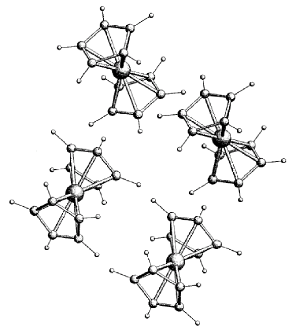
Figure 4.1: Crystalline structure of ferrocene, Fe(C₅H₅)₂ in its (room temperature) monociclic form with space group P2${}_{1}/a$. Two unit cells are included in the graph.

one can select a pair of interacting spins, i.e. a ¹³C and its directly bonded ¹H, arising on a molecule with a particular orientation. This is because the cyclopentadienyl rings perform fast thermal rotations ($\approx\operatorname{ps}$) around the five-fold symmetry axis, leading to a time averaged ¹³C-¹H interaction. The new dipolar constant depends [Sli92] only on the angle $\theta$ between the molecular axis and the external magnetic field $H_{0}$ and the angles between the internuclear vectors and the rotating axis, which in this case are $90^{\circ}$. Thus, the effective coupling constant is

$$b=\frac{1}{2}\frac{\mu_{0}\ \gamma_{\mathrm{H}}\,\gamma_{\mathrm{C}}\,\hbar^{2}}{4\pi r_{\mathrm{HC}}^{3}}\frac{\left\langle 3\cos^{2}\theta-1\right\rangle}{2},$$ (4.1)

where $\gamma$’s are the gyromagnetic factors and $r_{\mathrm{HC}}$ the internuclear distance. Notice that $b(\theta)$ cancels out at the magic angle $\theta_{\mathrm{m}}\simeq 54.74^{\circ}.$ As the chemical shift anisotropy of ¹³C is also averaged by the rotation and also depends on $\theta$ as $\left\langle 3\cos^{2}\theta-1\right\rangle,$ it is straightforward to assign each frequency in the ¹³C spectrum to a dipolar coupling $b$. Thus, all possible $b$ values are present in a single polycrystalline spectrum. The swapping induced by $b$ is turned on during the “contact time” $t_{\mathrm{c}}$, when the sample is irradiated with two radio frequencies fulfilling the Hartmann-Hahn condition [HH62, Sli92]. At $t=0,$ there is no polarization at ¹³C while the ¹H system is polarized. The polarization is transferred forth and back in the ¹³C-¹H pairs while the other protons inject polarization into these pairs. We show the raw experimental data of ¹³C polarization as a function of the contact time and $b(\theta)$ in fig. 4.2 a).

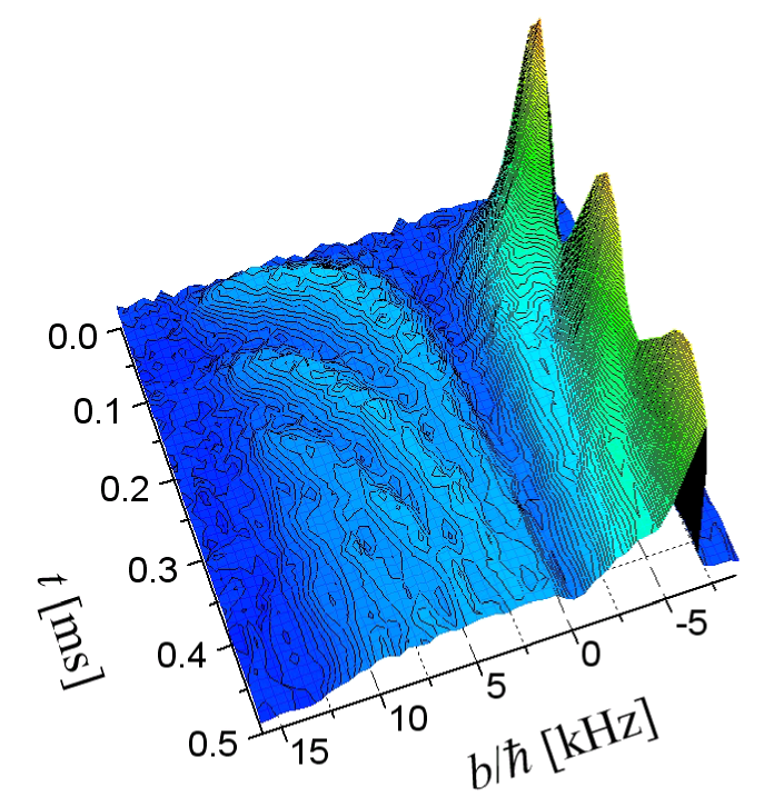
Figure 4.2: Raw experimental data of ¹³C polarization as a function of the contact time and spin-spin coupling $b(\theta)$ for a spin swapping dynamics in a ¹³C-¹H system.

In fig. 4.3 a), the polarizations have been normalized to their respective values at the maximum contact time ($3\operatorname{ms}$) for each $\theta$ when it saturates. It can be appreciated in the figure that the oscillation frequency is roughly proportional to $\left|b\right|,$ showing that this is the dominant interaction in the dynamics. This is consistent with the fact that the next ¹³C-¹H coupling strength with a non-directly bonded proton is roughly $b/8$ and, as all the intramolecular interactions, also scales with the angular factor $\left\langle 3\cos^{2}\theta-1\right\rangle$.

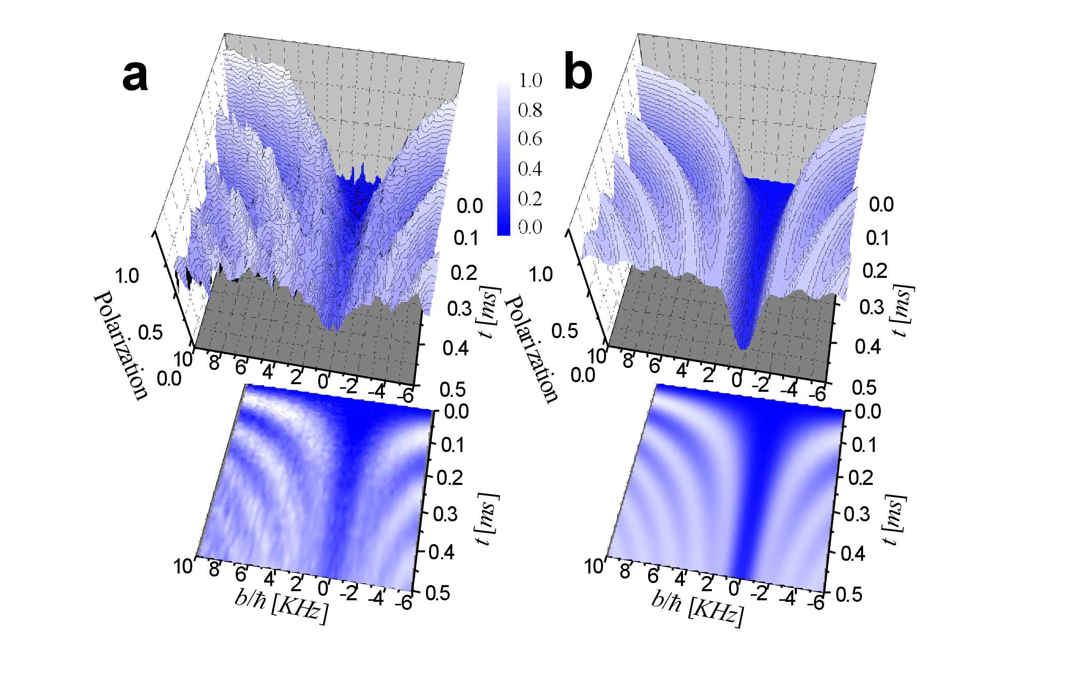
Figure 4.3: Spin swapping dynamics in ¹³C-¹H. a): Experimental ¹³C polarization in Fe(C₅H₅)₂ as a function of the contact time $t_{\mathrm{c}}$ and spin-spin coupling $b(\theta)$. b): Numerical simulations of the ¹³C polarization obtained from eq. (4.12) for different values of $b$, a dipolar system-environment interaction $\left(\left|a_{12}/b_{12}\right|=2\right)$ and a constant value for $\tau_{\mathrm{SE}}$ ($\tau_{\mathrm{SE}}=0.275\operatorname{ms}$) obtained by fitting the experimental data in the regime where the MKBE expression is valid. Projection plots in the $b-t$ plane show a canyon where the oscillation period diverges indicating a Quantum Dynamical Phase Transition.

A noticeable feature in these experimental data is the presence of a “canyon”, in the region $\left|b\right|<2\operatorname{kHz}$, where oscillations (swapping) disappear. The white hyperbolic stripes in the contour plot at the bottom evidence a swapping period $2\pi/\omega$ that diverges for a non-zero critical interaction. This divergence is the signature of a critical behavior.

The standard procedure to characterize the cross-polarization experiment in ferrocene and similar compounds was described in section § 2.1.2 that is derived from the MKBE model [MKBE74]. There the ¹³C polarization exchanges with that of its directly bonded ¹H, which, in turn, interacts isotropically with other protons that constitute the environment. Their solution is (3.111)

$$P^{{}^{\mathrm{MKBE}}}(t)=1-\frac{1}{2}\exp\left[-\frac{t}{\tau_{\phi}}\right]-\frac{1}{2}\cos(\omega t)\exp\left[-\frac{3}{2}\frac{t}{\tau_{\phi}}\right]),$$ (4.2)

where the decoherence rate becomes determined by the rate of interaction with the environment $\frac{1}{2}\Gamma_{\mathrm{SE}}/\hbar=1/\left(4\tau_{\mathrm{SE}}\right)\rightarrow 1/\tau_{\phi}\equiv R,$ while the swapping frequency is given by the two-spin dipolar interaction, $b/\hbar\rightarrow\omega$. A dependence of the inputs $b$ and $\tau_{\mathrm{SE}}$ on $\theta$ should manifest in the observables $\omega$ and $\tau_{\phi}.$ However, working on a polycrystal, each $\tau_{\mathrm{SE}}(\theta)$ value involves a cone of orientations of neighboring molecules and a rough description with single average value for the SE interaction rate is suitable.

We have performed non-linear least square fittings of the experimental points to the equation $P^{{}^{\mathrm{MKBE}}}(t)$ for the whole ¹³C spectra of ferrocene in steps of $\approx 80\operatorname{Hz}$ and contact times ranging from $2\operatorname{\mu s}$ to $3\operatorname{ms}$. The $1/\tau_{\phi}$ and $\omega$ parameters obtained from these fits are shown as dots in fig. 4.4. The proportionality of the frequency with $b$ for orientations that are far from the magic angle is verified. In this region a weak variation of $1/\tau_{\phi}$ around $2.2\operatorname{kHz}$ reflects the fact that $1/\left(2\tau_{\mathrm{SE}}\right)$ does not depend on $\theta$. A drawback of this simple characterization is that it tends to overestimate the width of the canyon because of limitations of the fitting procedure when eq. (4.2) is used around the magic angle.

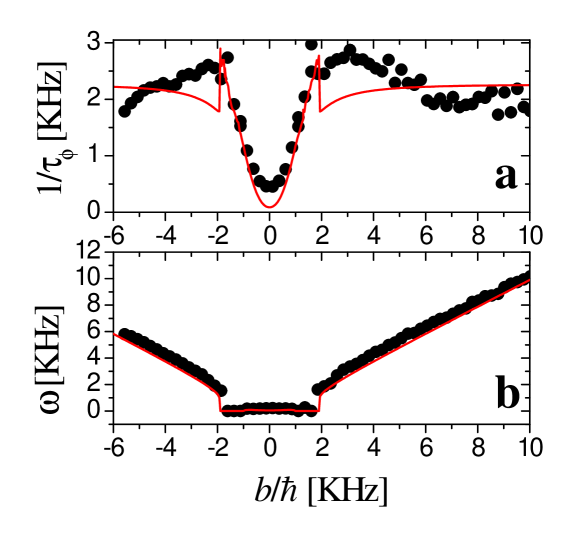
Figure 4.4: Decoherence rate $1/\tau_{\phi}$ and frequency $\omega$ in the spin swapping of a ¹³C-¹H system. Data points are obtained by fitting cross polarization experiments to the expression $P^{{}^{\mathrm{MKBE}}}(t)$. The zero plateau in the frequency and the parabolic behavior of $1/\tau_{\phi}$ in the region $b\tau_{\mathrm{SE}}\ll\hbar$ are indicative of an over-damped Zeno phase. Solid lines are the prediction of our model assuming a constant $\tau_{\mathrm{SE}}=0.275\operatorname{ms}$.

In spite of the MKBE theoretical prediction, one observes that the frequency becomes zero abruptly and the relaxation rate suddenly drops with a quadratic behavior when $b_{\mathrm{c}}\simeq 2\operatorname{kHz}$. The minimum of the parabola occurs at the magic angle, when $b=0.$ Then, all the polarization reaching the ¹³C at this orientation originates from protons outside the molecule. Then, the rate of $0.5\operatorname{kHz}$ obtained at this minimum constitutes an experimental estimation of this mechanism. This has to be compared with the almost constant value of $1/(4\tau_{\mathrm{SE}})=1/\tau_{\phi}\simeq 2.2\operatorname{kHz}$ observed outside the magic angle neighborhood. This justifies neglecting the $J$-coupling and the direct relaxation of the ¹³C polarization through the dipolar interaction with protons outside the molecule. In the following we describe our stroboscopic model that accounts for the “anomalous” experimental behavior.

4.2 Theoretical description

4.2.1 The system

Let us consider $M$ coupled $1/2$ spins with a Hamiltonian:

$$\widehat{\mathcal{H}}=\widehat{\mathcal{H}}_{\mathrm{Z}}+{\textstyle\sum\limits_{i<j}}\left[a_{ij}\hat{I}_{i}^{z}\hat{I}_{j}^{z}+b_{ij}\left(\hat{I}_{i}^{+}\hat{I}_{j}^{-}+\hat{I}_{i}^{-}\hat{I}_{j}^{+}\right)/2\right],$$ (4.3)

where

$$\mathcal{H}_{\mathrm{Z}}=\sum_{i=1}^{M}\hbar\left(\Omega_{\mathrm{Z}}+\delta\Omega_{i}\right)I_{i}^{z}$$ (4.4)

is the Zeeman energy, with a mean Larmor frequency $\Omega_{\mathrm{Z}}$. As we mention in previous chapters, the second term is the spin-spin interaction: $b_{ij}/a_{ij}=0$ is Ising, and $a_{ij}/b_{ij}=0,1,-2$ gives an $XY$, an isotropic (Heisenberg) or the truncated dipolar (secular), respectively.

In order to describe the experimental system, we use the model described in sections § 2.1.2 and § 3.4. Hence, let us take the first $N=2$ spins, $I_{0}\equiv S$ (a ¹³C) and $I_{1}$ (its directly bonded ¹H), as the “system” where the swapping $\left|\downarrow,\uparrow\right\rangle\rightleftarrows\left|\uparrow,\downarrow\right\rangle$ occurs under the action of $b_{01}$. The other $M-N$ spins (all the other ¹H), with $M\rightarrow\infty$, are the spin-bath or “environment”. This limit enables the application of the Fermi Golden Rule or a more sophisticated procedure to obtain a meanlife $\tau_{\mathrm{SE}}$ for the system levels. We will not need much detail for the parameters of the spin-bath in eq. (4.3) except for stating that it is characterized by an energy scale $d_{\mathrm{B}}$ which leads to a very short correlation time $\tau_{\mathrm{B}}\simeq\hbar/d_{\mathrm{B}}$. Thus, this spin system can be mapped into a fermion particle system using the Jordan-Wigner transformation [LSM61] as we described in section § 3.4. Under the experimental conditions, $\delta\Omega_{i}=0,$ $a_{01}=0$ and $b_{01}=b,$ the system Hamiltonian becomes (3.100)

$$\widehat{\mathcal{H}}_{\mathrm{S}}=\hbar\Omega_{\mathrm{Z}}\left(\hat{c}_{0}^{+}\hat{c}_{0}+\hat{c}_{1}^{+}\hat{c}_{1}-\hat{1}\right)+\tfrac{1}{2}b\left(\hat{c}_{0}^{+}\hat{c}_{1}+\hat{c}_{1}^{+}\hat{c}_{0}\right).$$ (4.5)

The Jordan-Wigner transformation maps a linear many-body $XY$ spin Hamiltonian into a system of non-interacting fermions. Spins $I_{i}$ with $2\leq i\leq M-1$ are interacting among them. To simplify the presentation, and without loss of generality, we consider a single connection between the system and the spin-bath $a_{1j}=b_{1j}=0,$ $j=3\ldots\infty$ and $a_{0j}=b_{0j}=0,$ $j=2\ldots\infty$ to use the SE interaction described by eq. (3.102)

$$\widehat{\mathcal{H}}_{\mathrm{SE}}=a_{12}\left(\hat{c}_{1}^{+}\hat{c}_{1}-\tfrac{1}{2}\right)\left(\hat{c}_{2}^{+}\hat{c}_{2}-\tfrac{1}{2}\right)+\tfrac{1}{2}b_{12}\left(\hat{c}_{1}^{+}\hat{c}_{2}+\hat{c}_{2}^{+}\hat{c}_{1}\right).$$ (4.6)

In the experimental initial condition, all spins are polarized with the exception of $S$ [MKBE74] (see section § 2.1.2). Thus in the high temperature limit ($\hbar\Omega_{\mathrm{Z}}/k_{\mathrm{B}}T\equiv s\ll 1$), the reduced density operator is

$$\hat{\sigma}\left(0\right)=\frac{\hbar}{\mathrm{i}}\hat{G}^{<}\left(0\right)=\left(\hat{1}+s\hat{I}_{1}^{z}\right)/\operatorname{Tr}\left\{\hat{1}\right\}$$ (4.7)

which under the Jordan-Wigner transformation becomes

$$\frac{\left(1-s/2\right)}{\operatorname{Tr}\left\{\hat{1}\right\}}\hat{1}+\frac{s}{\operatorname{Tr}\left\{\hat{1}\right\}}\hat{c}_{1}^{+}\hat{c}_{1}.$$ (4.8)

Since the first term does not contribute to the dynamics (§ 3.4), we retain only the second term and normalize it to the occupation factor. This means that site $1$ is empty while site $2$ and sites at the particle reservoir are “full”. This describes the tiny excess $\Delta p$ above the mean occupation $1/2$. To find the dynamics of the reduced density matrix of the “system”

$$\hat{\sigma}\left(t\right)=\frac{\hbar}{\mathrm{i}}\hat{G}^{<}\left(t\right),$$ (4.9)

we will take advantage of the particle representation and use the integral form [Kel64, Dan84] of the Keldysh formalism, eq. (3.20), instead of the standard Liouville-von Neumann differential equation, eq. (2.39), as we described in section § 3.4. There, any perturbation term is accounted to infinite order ensuring the proper density normalization. The interaction with the bath is local and, because of the fast dynamics in the bath, it can be taken as instantaneous [DÁLP07, ÁDLP07a]. Hence, the evolution is further simplified into an integral form of the Generalized Landauer Büttiker Equation (GLBE) [Pas91, Pas92] for the particle density [DÁLP07, ÁDLP07a]. There, the environment plays the role of a local measurement apparatus § 3.3.1.

4.2.2 Analytical solution

After all these assumption, we have the spin system used in section § 3.4 where we apply the spin-fermion mapping to use the Keldysh formalism. In that section, we obtain that the observable dynamics is consequence of a initial local excitation on site $1,$

$$G_{ij}^{<\left(1\right)}(0,0)=\tfrac{\mathrm{i}}{\hbar}\delta_{i1}\delta_{1j},$$ (4.10)

and evolve in the $1$-st particle subspace,

$$P_{i1}(t)=\tfrac{\hbar}{\mathrm{i}}G_{ii}^{<\,_{(1)}}(t,t).$$ (4.11)

After that, the solution of the polarization $P_{01}(t)$ (experimental ¹³C polarization) is the same that was obtained in (3.68),

$$P_{01}(t)=1-a_{0}e^{-R_{0}t}-a_{1}\cos\left[\left(\omega+\mathrm{i}\eta\right)t+\phi_{0}\right]e^{-R_{1}t},$$ (4.12)

where $V_{01}=-\frac{b}{2},~{}V_{ij}=-\tfrac{b_{ij}}{2}$, $U_{12}^{\mathrm{(dir.)}}=a_{12}$ and $U_{12}^{\mathrm{(ex.)}}=0$ and we substitute in the present solution $\Gamma_{\mathrm{XY}}\leftrightarrow\Gamma_{V},$ $\Gamma_{\mathrm{ZZ}}\leftrightarrow\Gamma_{U}$ and $p_{\mathrm{XY}}\leftrightarrow p_{V}.$ In spite of appearance, the last equation has a single fitting parameter. This is because the real functions $\omega,$ $\eta,$ $R_{0}$ and $R_{1}$ as well as $a_{0}$, $a_{1}$ and $\phi_{0}$ depend exclusively on $b,$ $\tau_{\mathrm{SE}}$ and $p_{\mathrm{XY}}$. Besides, $b$ and $p_{\mathrm{XY}}$ are determined from crystallography and the anisotropy of the magnetic interaction ($p_{\mathrm{XY}}=1/5$ for dipolar) respectively. The phase transition is ensured by the condition $\omega\eta\equiv 0$. The anisotropy ratio $\Gamma_{\mathrm{XY}}/\Gamma_{\mathrm{SE}}\rightarrow p_{\mathrm{XY}}$ accounts for the observed competition (see section § 2.1.2 and § 2.2.2.1) between the Ising and XY terms of $\widehat{\mathcal{H}}_{\mathrm{SE}}$. The Ising interaction drives the “system” to the internal quasi-equilibrium (2.63). In contrast, the XY term allows the thermal equilibration with the bath [CÁL⁺03].

4.2.3 Comparison with the experiments

In order to see how well our model reproduces the experimental behavior we plot the ¹³C polarization with realistic parameters. Since the system is dominated by the dipolar SE interaction [CÁL⁺03], as we described in chapter 2 we take $\left|a_{12}/b_{12}\right|=2.$ We introduce $b$ with its angular dependence according to eq. (4.1) and we select a constant value for $\tau_{\mathrm{SE}}=0.275\operatorname{ms}$ representative of the $b\gg\hbar/\tau_{\mathrm{SE}}$ regime. Since here, we are only interested in the qualitative aspects of the critical behavior of the dynamics, there is no need to introduce $\tau_{\mathrm{SE}}(\theta)$ as a fitting parameter. These evolutions are normalized at the maximum contact time ($3\operatorname{ms}$) experimentally acquired. They are shown in fig. 4.3 b) where the qualitative agreement with the experimental observation of a canyon is evident. Notice that the experimental canyon is less deep than the theoretical one. This is due to intermolecular ¹³C-¹H couplings neglected in the model. We will show that the analytical expression of eq. (4.12) allows one to determine the edges of the canyon which are the critical points of what we will call a Quantum Dynamical Phase Transition (QDPT).

4.3 Quantum Dynamical Phase Transition

Our quantum observable (the local spin polarization) is a binary random variable. The dynamics of its ensemble average (swapping probability), as described by eq. (4.12), depends parametrically on the “noisy” fluctuations of the environment through $\tau_{\mathrm{SE}}$. Thus, following Horsthemke and Lefever [HL84], one can identify the precise value for $\tau_{\mathrm{SE}}$ where a qualitative change in the functional form of this probability occurs as the critical point of a phase transition. This is evidenced by the functional change (nonanalyticity) of the dependence of the observables (e.g. the swapping frequency $\omega$) on the control parameter $b\tau_{\mathrm{SE}}/\hbar$. Since the control parameter switches among dynamical regimes we call this phenomenon a Quantum Dynamical Phase Transition.

It should be remarked that the effect of other spins on the two spin system introduces non-commuting perturbing operators (symmetry breaking perturbations) which produce non-linear dependences of the observables. While this could account for cross-over among the limiting dynamical regimes, it does not ensure a phase transition. A true phase transition needs a non-analyticity in these functions which is only enabled by taking the thermodynamic limit of an infinite number of spins [Sac01]. In our formalism, this is incorporated through the imaginary part of the energy, $\hbar/\tau_{\mathrm{SE}}$, evaluated from the Fermi Golden Rule (3.19).

When the SE interaction rates are anisotropic ($\Gamma_{\mathrm{ZZ}}\neq\Gamma_{\mathrm{XY}}$), there is a functional dependence of $\omega\$on $\tau_{\mathrm{SE}}$ and $b$ yielding a critical value for their product, $b\tau_{\mathrm{SE}}/\hbar=k_{p_{\mathrm{XY}}},$ where the dynamical regime switches. One identifies two parametric regimes: 1- The swapping phase, which is a form of sub-damped dynamics, when $b\tau_{\mathrm{SE}}/k_{p_{\mathrm{XY}}}>\hbar$ ($\eta=0$ in eq. (4.12)). 2- A Zeno phase, with an over-damped dynamics for $b\tau_{\mathrm{SE}}/k_{p_{\mathrm{XY}}}<\hbar$ as a consequence of the strong coupling with the environment (zero frequency, i.e. $\omega=0$, in eq. (4.12)). In the neighborhood of the critical point the swapping frequency takes the form:

$$\omega=\left\{\begin{array}[c]{cc}a_{p_{\mathrm{XY}}}\sqrt{\left(b/\hbar\right)^{2}-k_{p_{\mathrm{XY}}}^{2}/\tau_{\mathrm{SE}}^{2}}&b\tau_{\mathrm{SE}}/k_{p_{\mathrm{XY}}}>\hbar\\ 0&b\tau_{\mathrm{SE}}/k_{p_{\mathrm{XY}}}\leq\hbar\end{array}\right..$$ (4.13)

and $\eta$ becomes

$$\eta=\left\{\begin{array}[c]{cc}0&b\tau_{\mathrm{SE}}/k_{p_{\mathrm{XY}}}>\hbar\\ a_{p_{\mathrm{XY}}}\sqrt{k_{p_{\mathrm{XY}}}^{2}/\tau_{\mathrm{SE}}^{2}-\left(b/\hbar\right)^{2}}&b\tau_{\mathrm{SE}}/k_{p_{\mathrm{XY}}}\leq\hbar\end{array}\right.,$$ (4.14)

where

$$k_{p_{\mathrm{XY}}}^{2}=\frac{1}{12}\left\{\left[\left(p_{\mathrm{XY}}-1\right)^{2}\chi\left(p_{\mathrm{XY}}\right)\right]^{\frac{1}{3}}+\zeta\left(p_{\mathrm{XY}}\right)+19p_{\mathrm{XY}}^{2}+\frac{\left(p_{\mathrm{XY}}-1\right)^{\frac{4}{3}}\zeta\left(p_{\mathrm{XY}}\right)}{\left[\chi\left(p_{\mathrm{XY}}\right)\right]^{\frac{1}{3}}}\right\},$$ (4.15)

$$\chi\left(p_{\mathrm{XY}}\right)=-5291p_{\mathrm{XY}}^{4}-1084p_{\mathrm{XY}}^{3}+546p_{\mathrm{XY}}^{2}-4p_{\mathrm{XY}}+1+24\sqrt{3}p_{\mathrm{XY}}\sqrt{\left(28p_{\mathrm{XY}}^{2}-2p_{\mathrm{XY}}+1\right)^{3}},$$ (4.16)

$$\zeta\left(p_{\mathrm{XY}}\right)=-215p_{\mathrm{XY}}^{2}-2p_{\mathrm{XY}}+1,$$ (4.17)

and

$$a_{p_{\mathrm{XY}}}^{2}=\frac{1}{2}\frac{\left(f_{1}^{~{}~{}2/3}+36f_{2}\right)\left(-f_{3}f_{1}^{\ \ 2/3}+36f_{2}f_{3}+f_{1}f_{4}\right)}{f_{1}^{~{}~{}5/3}f_{4}},$$ (4.18)

$$f_{1}=36k_{p_{\mathrm{XY}}}^{2}-8+24p_{\mathrm{XY}}+48p_{\mathrm{XY}}^{2}-36k_{p_{\mathrm{XY}}}^{2}p_{\mathrm{XY}}-64p_{\mathrm{XY}}^{3}+12f_{4},$$ (4.19)

$$f_{2}=1/3k_{p_{\mathrm{XY}}}^{2}-1/3p_{\mathrm{XY}}^{2}-1/9\left(1-p_{\mathrm{XY}}\right)^{2},$$ (4.20)

$$f_{3}=-f_{4}+p_{\mathrm{XY}}f_{4}-6k_{p_{\mathrm{XY}}}^{2}-16p_{\mathrm{XY}}^{4}+20p_{\mathrm{XY}}^{3}-10p_{\mathrm{XY}}^{2}+13p_{\mathrm{XY}}^{2}k_{p_{\mathrm{XY}}}^{2}-2k_{p_{\mathrm{XY}}}^{2}p_{\mathrm{XY}}+k_{p_{\mathrm{XY}}}^{2},$$ (4.21)

$$f_{4}=\left(12k_{p_{\mathrm{XY}}}^{2}+96p_{\mathrm{XY}}^{4}k_{p_{\mathrm{XY}}}^{2}-120p_{\mathrm{XY}}^{3}k_{p_{\mathrm{XY}}}^{2}+60p_{\mathrm{XY}}^{2}k_{p_{\mathrm{XY}}}^{2}-39k_{p_{\mathrm{XY}}}^{2}p_{\mathrm{XY}}^{2}\right.\\ \left.+6k_{p_{\mathrm{XY}}}^{2}p_{\mathrm{XY}}-3k_{p_{\mathrm{XY}}}^{2}-48p_{\mathrm{XY}}^{4}+48p_{\mathrm{XY}}^{3}-12p_{\mathrm{XY}}^{2}\right)^{\frac{1}{2}}.$$ (4.22)

In equation (4.18) the functions $f_{1},$ $f_{2},$ $f_{3}$ and $f_{4}$ only depend of $p_{\mathrm{XY}}.$ Thus, the parameters $a_{p_{\mathrm{XY}}}$ and $k_{p_{\mathrm{XY}}}$ only depend on $p_{\mathrm{XY}}$ which is determined by the origin of the interaction Hamiltonian. For typical interaction Hamiltonians the values of these parameters $\left(p_{\mathrm{XY}},k_{p_{\mathrm{XY}}},a_{p_{\mathrm{XY}}}\right)$ are: Ising $\left(0,\frac{1}{2},1\right)$, dipolar $\left(\frac{1}{5},0.3564,0.8755\right)$, isotropic $\left(\frac{1}{2},0,\frac{1}{\sqrt{2}}\right)$ and $XY$ $\left(1,1,1\right)$. Fig. 4.5

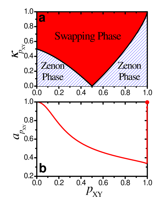
Figure 4.5: a) Critical value of the swapping frequency as a function of $p_{\mathrm{XY}}$ (anisotropy of the SE interaction). b) The parameter $a_{p_{\mathrm{XY}}}$ of the swapping frequency as a function of $p_{\mathrm{XY}}.$

shows the parameters $a_{p_{\mathrm{XY}}}$ and $\kappa_{p_{\mathrm{XY}}}$ as a function of $p_{\mathrm{XY}}$. It is important to note that when the SE interaction rates are isotropic ($\Gamma_{\mathrm{XY}}=\Gamma_{\mathrm{ZZ}}$) the critical point is zero, thus, the oscillation frequency is finite for all values of the SE interaction rate $\Gamma_{\mathrm{SE}}/\hbar$. While the oscillation could be very attenuated it is ensured a swapping with a frequency proportional to $b.$ The swapping period is

$$T\simeq\frac{T_{0\mathrm{c}}^{3/2}}{\sqrt{2}a_{p_{\mathrm{XY}}}}\ \left(T_{0\mathrm{c}}-T_{0}\right)^{-1/2},$$ (4.23)

where

$$T_{0}=\frac{2\pi\hbar}{b}$$ (4.24)

is the isolated two spin period and its critical value

$$T_{0\mathrm{c}}=\frac{2\pi\tau_{\mathrm{SE}}}{k_{p_{\mathrm{XY}}}},$$ (4.25)

determines the region where the period $T$ diverges as is observed in fig. 4.3. The estimated value of $\tau_{\mathrm{SE}}=0.275\operatorname{ms}$ and dipolar SE interactions yield a critical value for the ¹³C-¹H coupling of $b_{\mathrm{c}}/\hbar=2\pi/T_{0\mathrm{c}}=1.3\operatorname{kHz}\mathrm{.}$

The complete phase diagram that accounts for the anisotropy of the SE interactions is shown in fig. 4.6. There, the frequency dependence on $p_{\mathrm{XY}}$ and $b\tau_{\mathrm{SE}}/\hbar$ is displayed. At the critical line, $k_{p_{\mathrm{XY}}}^{2}$ as a function of $p_{\mathrm{XY}},$ the frequency becomes zero setting the limits between both dynamical phases.

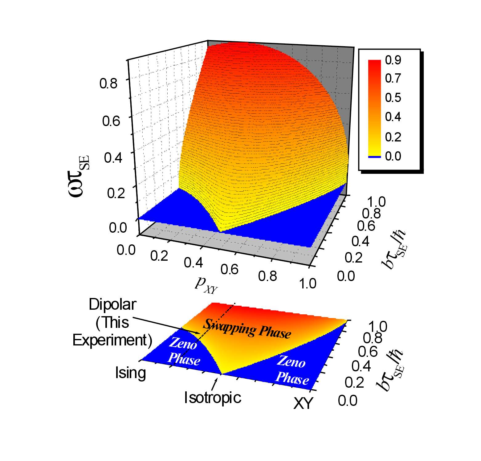
Figure 4.6: Quantum dynamical phase diagram for the spin swapping operation. The figure shows the frequency dependence on system-environment (SE) interaction anisotropy $p_{\mathrm{XY}}$ and the ratio among the internal and the SE interaction $b\tau_{\mathrm{SE}}/\hbar$. The projection over the $b\tau_{\mathrm{SE}}/\hbar-p_{\mathrm{XY}}$ plane determines the phase diagram where the transition between the swapping phase into the Zeno phase ($\omega=0)$ is manifested. Values of $p_{\mathrm{XY}}$ for typical SE interaction Hamiltonian are indicated in the contour plot.

The two dynamical phases can now be identified in the NMR experiments which up to date defied explanation. The experimental setup provides a full scan of the parameter $b\tau_{\mathrm{SE}}$ through the phase transition that is manifested when the frequency goes suddenly to zero (fig. 4.4 b) and the relaxation rate [fig. 4.4 a)] changes its behavior decaying abruptly. The fact that $1/\tau_{\phi}$ tends to zero when $b\ll\hbar/\tau_{\mathrm{SE}}$ confirms the Zeno phase predicted by our model. In this regime, $1/\tau_{\phi}$ is quadratic on $b$ as prescribed by eq. (3.113),

$$1/\tau_{\phi}\propto\left(b/\hbar\right)^{2}\tau_{\mathrm{SE}}.$$ (4.26)

To make the comparison between the two panels of fig. 4.3 quantitative, we fit the predicted dynamics of fig. 4.3 b) with $P^{{}^{\mathrm{MKBE}}}\left(t\right),$ following the same procedure used to fit the experimental data. The solid line in fig. 4.4 show the fitting parameters $1/\tau_{\phi}$ and $\omega$ in excellent agreement with the experimental ones.

We point out that eq. (4.2) is used to fit both the experiments and the theoretical prediction of eq. (4.12) because it constitutes a simple, thought imperfect, way to extract the “outputs” (oscillation frequency $\omega$ and a decoherence time $\tau_{\phi}$). While the systematic errors shift the actual critical value of the control parameter, $b/\hbar$, from $1.3\operatorname{kHz}$ to $2\operatorname{kHz}$, eq. (4.2) yields a simplified way to “observe” the transition.

4.4 Signatures of a QDPT in a three-spin system coupled to a spin-bath

We consider a three-spin system with the following Hamiltonian

$$\widehat{\mathcal{H}}_{\mathrm{S}}=\hbar\Omega_{\mathrm{Z}}\left(\hat{I}_{-1}^{z}+\hat{I}_{0}^{z}+\hat{I}_{1}^{z}\right)+\tfrac{1}{2}b\left(\hat{I}_{-1}^{+}\hat{I}_{0}^{-}+\hat{I}_{-1}^{-}\hat{I}_{0}^{+}\right)+\tfrac{1}{2}b\left(\hat{I}_{0}^{+}\hat{I}_{1}^{-}+\hat{I}_{0}^{-}\hat{I}_{1}^{+}\right),$$ (4.27)

where we add one spin to the system. However, in this case there is not a interaction between the spin $I_{-1}$ and the $I_{1}$ as there was in section § 2.2. The environment Hamiltonian and the SE interaction Hamiltonians remain as in the previous section,

$$\widehat{\mathcal{H}}_{\mathrm{E}} =\sum_{i\geq 2}\hbar\Omega_{\mathrm{Z}}\hat{I}_{i}^{z}+{\textstyle\sum\limits_{\genfrac{}{}{0.0pt}{1}{i\geq 2}{j>i}}}\tfrac{1}{2}b_{ij}\left(\hat{I}_{i}^{+}\hat{I}_{j}^{-}+\hat{I}_{i}^{-}\hat{I}_{j}^{+}\right),$$ (4.28)

$$\widehat{\mathcal{H}}_{\mathrm{SE}} =a_{12}\hat{I}_{1}^{z}\hat{I}_{2}^{z}+\tfrac{1}{2}b_{12}\left(\hat{I}_{1}^{+}\hat{I}_{2}^{-}+\hat{I}_{1}^{-}\hat{I}_{2}^{+}\right).$$ (4.29)

Also, the environment is coupled only to one spin of the system. We solve the generalized quantum master equation (2.39), using the same procedure as in section § 2.1.2.2, without neglecting non-secular terms of the relaxation superoperator. Considering now the initial condition

$$\hat{\sigma}\left(0\right)=\frac{\left(\hat{1}+\beta_{\mathrm{B}}\hbar\Omega_{0,I}\hat{I}_{-1}^{z}\right)}{\mathrm{Tr}\left\{\hat{1}\right\}}$$ (4.30)

and the spin-bath polarized, we obtain for the magnetization of site $-1$

$$M_{I_{-1}^{z}}\left(t\right) =\mathrm{Tr}\left\{\hat{I}_{-1}^{z}\hat{\sigma}\left(t\right)\right\}$$ (4.31)

$$=M_{0}\left(1-a_{0}e^{-R_{0}t}-a_{1}e^{-R_{1}t}+a_{2}\mathop{\rm sen}\nolimits\left(\omega_{2}t+\phi_{2}\right)e^{-R_{2}t}+a_{3}\mathop{\rm sen}\nolimits\left(\omega_{3}t+\phi_{3}\right)e^{-R_{3}t}\right).$$ (4.32)

The coefficients $a_{i},$ $R_{i}$, $\omega_{i}$ and $\phi_{i}$ are real and they are functions of $b,$ $1/\tau_{\mathrm{SE}}\$and $p_{\mathrm{XY}}.$ If $p_{\mathrm{XY}}\neq 0$ the final state has all the spins polarized because a net transfer of magnetization from the spin-bath is possible. However, for an Ising SE interaction, $p_{\mathrm{XY}}=0,$ we obtain that $R_{0}=0$ and $1-a_{0}=1/3$ (the asymptotic polarization) because the final state is the quasi-equilibrium of the $3$-spin system as we described in section § 2.2.2.1, eq. (2.116). In fig. 4.7

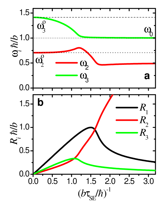
Figure 4.7: a) Frequencies involved in the temporal evolution of the polarization in the $3$-spin system as a function of $\left(b\tau_{\mathrm{SE}}/\hbar\right)^{-1}$. Dashed lines represent the isolated system. Dot line correspond to two spins decoupled from the environment. b) Different relaxation rates of the polarization.

we show the frequencies $\omega_{2}$ and $\omega_{3}$ and the different relaxation rates as a function of $\left(b\tau_{\mathrm{SE}}/\hbar\right)^{-1}$ when the SE interaction is Ising $(p_{\mathrm{XY}}=0)$. Two changes, each resembling the critical behavior shown by two spin systems are observed (see fig. 4.4). The same phenomenon occurs in figure 4.8 a)

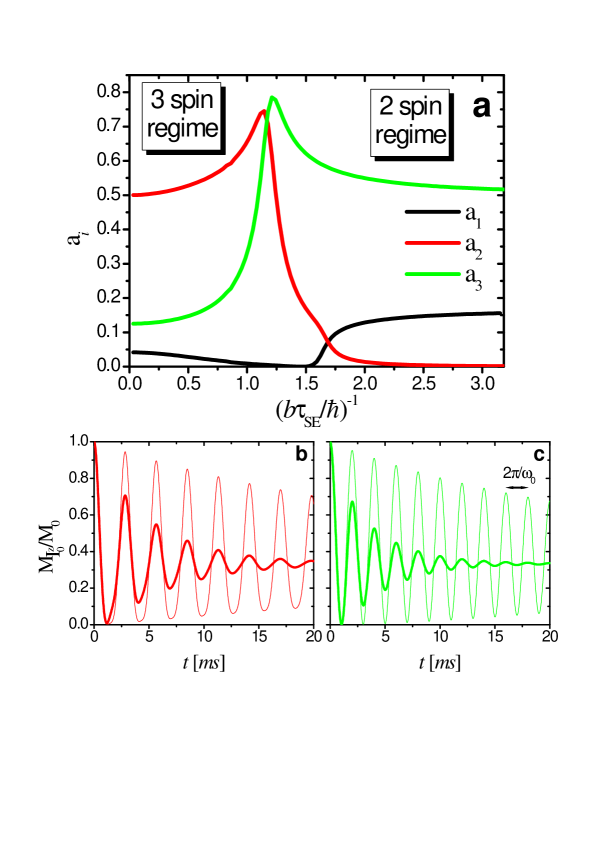
Figure 4.8: a) Coefficients (weights) of the different terms of eq. (4.31). At the critical region there is a switch between  the $2$-spin and the $3$-spin regime. b) and c) Temporal evolutions of the polarization in the $2$-spin and $3$-spin regimes respectively for different $\tau_{\mathrm{SE}}.$ In b) $b/\hbar=2\pi\times 1\operatorname{kHz}$ and $\tau_{\mathrm{SE}}=1.43\operatorname{ms}$ for the thick line and $\tau_{\mathrm{SE}}=10\operatorname{ms}$ for the thin line. In c) $b/\hbar=2\pi\times 1\operatorname{kHz}$ and $\tau_{\mathrm{SE}}=0.1\operatorname{ms}$ for the thick line and $\tau_{\mathrm{SE}}=0.01\operatorname{ms}$ for the thin line.

where the coefficients $a_{i}$ are shown. The polarization evolution of an isolated $3$-spin system is

$$M_{I_{-1}^{z}}\left(t\right)=\frac{M_{0}}{8}\left(3+4\cos\left(\omega_{2}^{o}t\right)+\cos\left(\omega_{3}^{o}t\right)\right)$$ (4.33)

where

$$\omega_{2}^{o}=\frac{\sqrt{2}}{4}\frac{b}{\hbar}$$ (4.34)

and

$$\omega_{3}^{o}=\frac{\sqrt{2}}{2}\frac{b}{\hbar}$$ (4.35)

are the natural frequencies. When $\left(b\tau_{\mathrm{SE}}/\hbar\right)^{-1}<<1,$ we observe that $\omega_{2}\rightarrow\omega_{2}^{o},$ $\omega_{3}\rightarrow\omega_{3}^{o},$ $a_{1}\rightarrow 1/3-3/8=-1/24,$ $a_{2}\rightarrow 1/2$ and $a_{3}\rightarrow 1/8$ as expected for an isolated $3$-spin dynamics. The dependence of $\omega_{3}$ as a function of $\left(b\tau_{\mathrm{SE}}/\hbar\right)^{-1}$ is similar to that of the swapping frequency of fig. 4.4. However, instead of becoming zero when the SE interaction increase, it suddenly stabilizes at $\omega_{0}=b/\hbar$, the bare $2$-spin Rabi frequency. At the same point $\omega_{2}$, $R_{2}$ and $R_{3}$ also have a sudden change. While $R_{2}$ and $R_{3}$ initially grew as $\left(b\tau_{\mathrm{SE}}/\hbar\right)^{-1}$, there $R_{2}$ increases the growing speed while $R_{3}$ begins to decay as in the Zeno phase (see fig. 4.4). Moreover, looking at the behavior of the coefficients $a_{2}$ and $a_{3}$, we observe a form of switch between them, $a_{2}$ suddenly goes down and $a_{3}$ goes up. These coefficients are the weight of the different frequency contributions in the time evolution. Both changes together, on the decoherence rates and on the weight coefficients of the different oscillatory terms, beyond the critical interaction (region) leads the system to oscillate with the bare Rabi frequency of the two spins decoupled from the environment. If we continue increasing the control parameter $\left(b\tau_{\mathrm{SE}}/\hbar\right)^{-1},$ this effect is enhanced by the next transition. After the second transition, $R_{1}$ begins to decrease as in the Zeno phase behavior of fig. 4.4. As the term of eq. 4.31 that relax with $R_{1}$ leads the system to the $3$-spin quasi-equlibrium, when it goes down this final state is approached more slowly. This effect tries to avoid the interaction between the $2$-spins not coupled to the environment and the $I_{2}$ spin. After the second transition, the coefficient $a_{1}$ goes to zero abruptly leading to a more pronounced “isolation” of the $2$-spins. After that, we can characterize two dynamical regimes: One which is characterized by the $3$-spin dynamics when $\left(b\tau_{\mathrm{SE}}/\hbar\right)^{-1}\lesssim 1$ and the second one, when $\left(b\tau_{\mathrm{SE}}/\hbar\right)^{-1}\gtrsim 1,$ have the $2$-spin behavior.

Fig. 4.8 b) and c) show the temporal evolution of the magnetization of eq. (4.31) on the $3$-spins and the $2$-spin regimes respectively. While in fig. 4.8 b) the two frequency contributions are evident, in fig. 4.8 c) only the bare Rabi frequency is manifested. In each graph we show two curves with different SE interactions. In fig. 4.8 b), we show that increasing the SE interaction the decoherence rates increase. However, in the $2$-spin regime [fig. 4.8 c)] when it is increased the decoherence rate decrease leading to a better “isolation”. It is important to take into account that while the relaxation rates goes to zero smoothly the swapping frequency acquire the bare value near the critical point. Another fact to remark is that this effect is more pronounced when the anisotropy of the SE interaction is close to a pure Ising SE interaction while an increase in the XY nature leads a further smoothing of the transition. The reason is that, when $p_{\mathrm{XY}}\neq 0$, there is a net transfer of magnetization to the system which is redistributed between the three spins, this redistribution begins to be slower at the second transition when $R_{3}$ goes down. In contrast, for a purely Ising interaction, there is no net polarization transfer and a purely decoherent process at site $3$ freezes its dynamics but its fast energy fluctuations prevent the interaction with the other spins.

4.5 Summary

We found experimental evidence that environmental interactions can drive a swapping gate through a Quantum Dynamical Phase Transition towards an over-damped or Zeno phase [ÁDLP06]. The NMR implementation of a spin swapping in a ¹³C-¹H system enables the identification and characterization of this phase transition as a function of the ratio $b\tau_{\mathrm{SE}}/\hbar$ between the internal and SE interaction. In chapter 3, we developed a microscopic model [DÁLP07, ÁDLP07a] that describes both phases and the critical region with great detail, showing that it depends only on the nature of the interaction [ÁDLP06, ÁDLP07a]. In particular, the phase transition does not occur if the SE interaction gives isotropic interaction rates, $\Gamma_{\mathrm{ZZ}}=\Gamma_{\mathrm{XY}}$. The phase transition is manifested not only in the observable swapping frequency but also in the decoherence rate $1/\tau_{\phi}$. While a perturbative estimation through the standard Fermi golden rule would tend to identify this rate with the SE interaction, i.e. $1/\tau_{\phi}\cong 1/\tau_{\mathrm{SE}}$ $\simeq\left(d_{23}/\hbar\right)^{2}\tau_{\mathrm{B}},$ as it occurs well inside the swapping phase, both rates differ substantially as the system enters in the Zeno phase ($b\tau_{\mathrm{SE}}\leq k_{p_{\mathrm{XY}}}\hbar$). Here, the decoherence rate switches to the behavior $1/\tau_{\phi}\propto\left(b/\hbar\right)^{2}\tau_{\mathrm{SE}}$. In the Zeno phase, the system’s free evolution decays very fast with a rate $\tau_{\mathrm{SE}}^{-1}$. In spite of this, one can see that the initial state as a whole has a slow decay (its dynamics becomes almost frozen) because it is continuously fed by the environment. Since the $\tau_{\mathrm{SE}}$ has become the correlation time for the spin directly coupled to the environment, $1/\tau_{\phi}$ provided by our calculation can be interpreted as a “nested” Fermi golden rule rate emphasizing the non-perturbative nature of the result [ÁDLP06]. Based on the wealth of this simple swapping dynamics, we can foresee applications that range from tailoring the environments for a reduction of their decoherence on a given process to using the observed critical transition in frequency and decoherence rate as a tracer of the environment’s nature. This led us to extend the model to a $3$-spin system and to show that beyond a critical region the two spins become almost decoupled from the environment oscillating with the bare Rabi frequency and relaxing more slowly [ÁLP07]. While in the two spin swapping gate the dynamical transition is critical, in the $3$-spin system the criticality is smoothed out. However, enough abruptness remains to give the possibility to use it to “isolate” a two-spin system with a finite system-environment interaction. Thus, these applications open new opportunities for both, the field of quantum information processing and the general physics and chemistry of open quantum systems [DÁLP07].

Chapter 5 Polarization transfer enhancement by selective pruning in NMR

Inspired in the stroboscopic model discussed in section § 3.3, we propose a new NMR pulse sequence to improve the transfer of polarization through a specific pathway in a system of many interacting spins. The sequence effectively prunes branches of spins, where no polarization is required, during the polarization transfer procedure. In this way, a local polarization excitation is transferred more efficiently from a chosen “source spin” to a “target spin”. Simulations of the spin dynamics with real values of chemical shifts and $J$-couplings in the ¹³C backbone of leucine for a couple of sources and targets are performed. Enhancements of a factor of up to $300\%$ in the target polarization are observed without sacrificing the relevant times. Possible applications and potential fundamental contributions to engineered decoherence are discussed.

5.1 The pruner sequence

One standard procedure to transfer polarization within molecules in the liquid state, called TOCSY (Total Correlation Spectroscopy) [BE83, BD85] is based on the isotropic interaction (or $J$-interaction). In general, one has a mixing Hamiltonian which makes possible the spin-spin interaction. The mixing Hamiltonian in the rotating frame for an isotropic interaction is

$$\widehat{\mathcal{H}}_{\mathrm{mix}}^{\mathrm{iso}}=\sum_{i\neq j}J_{ij}\left(\hat{I}_{i}^{z}\hat{I}_{j}^{z}+\hat{I}_{i}^{y}\hat{I}_{j}^{y}+\hat{I}_{i}^{x}\hat{I}_{j}^{x}\right),$$ (5.1)

where $J_{ij}$ is the scalar coupling and $\hat{I}_{i}^{u}$ $\left(u=x,y,z\right)$ are the spin operators. As this Hamiltonian connects all the possible pairs of spins, an initial local excitation would spread over all of them. The idea behind our new sequence is to effectively “disconnect” those spins which do not belong to the “selected transfer pathway”. In order to achieve this goal, one makes use of the differences in chemical shifts in the spin system.

“The pruner” sequence stroboscopically interrupts the mixing evolution performed under $\widehat{\mathcal{H}}_{\mathrm{mix}}^{\mathrm{iso}}$ with free evolutions, that in the rotating frame are given by

$$\widehat{\mathcal{H}}_{\mathrm{free}}=\sum_{i}\hbar\Delta\Omega_{i}\hat{I}_{i}^{z}+\sum_{i\neq j}J_{ij}\hat{I}_{i}^{z}\hat{I}_{j}^{z},$$ (5.2)

where $\Delta\Omega_{i}$ are the off-resonance shifts as defined in 2.7 and $\Delta_{ij}=\hbar(\Delta\Omega_{i}-\Delta\Omega_{j})\gg J_{ij}$. Thus, there is a time interval, $\Delta t_{\mathrm{mix}},$ with the mixing evolution under the Hamiltonian $\widehat{\mathcal{H}}_{\mathrm{mix}}^{\mathrm{iso}}$ followed by a free evolution time step $\Delta t_{\mathrm{free}}$. This sequence of evolutions are repeated successively as schematized in fig. 5.1.

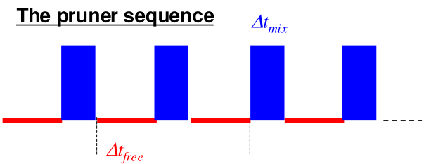
Figure 5.1: Schematic representation of the pruner sequence.

The adjustment of the free evolution time, $\Delta t_{\mathrm{free}}$, must be a least common multiple of the inverses of the chemical shift differences

$$\Delta_{ij}=\hbar\left(\Delta\Omega_{i}-\Delta\Omega_{j}\right)$$ (5.3)

between the spins connected in the pathway, i.e.

$$\Delta t_{\mathrm{free}}=2\pi n_{ij}\hbar/\left|\Delta_{ij}\right|$$ (5.4)

where $n_{ij}$ is a natural number. Thus, all the spins in the pathway are in phase because their relative phase is proportional to $2\pi$, while the others are dephased in each free evolution.

5.2 Numerical simulation on the L-leucine molecule

Simulations of a local excitation dynamics under “the pruner” sequence were performed for different topologies and initial conditions. The topologies, chemical shifts and $J$-couplings to exemplify the operation of the sequence were extracted from amino acid molecules. Here, we present the simulations that were done in the L-leucine molecule (see fig. 5.2).

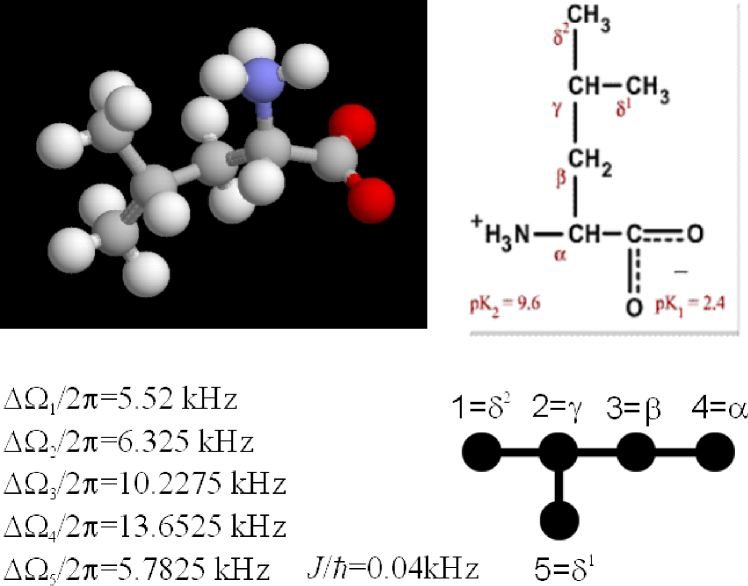
Figure 5.2: Molecule of L-leucine showing the numbering of the carbons used in the spin dynamics calculation. The carboxylate carbon is not considered in the simulations because as it resonates at quite different frequency is easily decoupled from the others. The ¹³C chemical shifts in a $23\operatorname{T}$  magnet at pH $6.89$ are $\Delta\Omega_{1}/2\pi=5.52\operatorname{kHz}\mathrm{,}$ $\Delta\Omega_{2}=6.325\operatorname{kHz}$, $\Delta\Omega_{3}=10.2275\operatorname{kHz}\mathrm{,}$ $\Delta\Omega_{4}=13.6525\operatorname{kHz}$ and $\Delta\Omega_{5}=5.7825\operatorname{kHz}\mathrm{,}$ and $J/\hbar=0.04\operatorname{kHz}\mathrm{\ }$for all the ¹³C-¹³C nearest neighbor couplings.

We find that the pruning is more effective for

$$\Delta t_{\mathrm{mix}}\ll\hbar/J_{ij}^{\mathrm{path}}$$ (5.5)

where $J_{ij}^{\mathrm{path}}$ are the $J$-couplings in the pathway. However, polarization transfer becomes much slower than in a regular isotropic mixing sequence. Thus, after numerical explorations, we found that for a practical experimental situation, a good compromise for an enhancement of the signal is found if the time interval for evolution under $\widehat{\mathcal{H}}_{\mathrm{mix}}^{\mathrm{iso}}$ is

$$\Delta t_{\mathrm{mix}}\sim\frac{1}{10}\left(\hbar/J_{ij}^{\mathrm{path}}\right).$$ (5.6)

This allows one to observe a polarization transfer that is larger than the one obtained by the isotropic mixing. In general, for arbitrary chemical shift differences $\Delta_{ij},$ it is difficult to obtain a short time $\Delta t_{\mathrm{free}}$. Then, one must find an approximate solution to avoid excessive long times. Therefore, the particular enhancement factor depends on the number of spins necessary to reach the target: the more spin steps the lower efficiency of the overall sequence. In pathways with three spins, the enhancement factor in the polarization transfer is approximately three. In the case of a completely enriched carbon-13 backbone of an L-leucine residue (fig. 5.3)

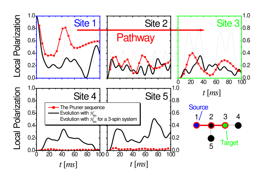
Figure 5.3: Local polarization evolution under the pruner sequence at different ¹³C sites in L-leucine. The initial local excitation at site $1$ (the source) is transfered through the selected pathway ($1-2-3$), to site $3.$ The free evolution time is $\Delta t_{\mathrm{free}}=1.2744\operatorname{ms}=6\times\hbar/\Delta_{13}\approx\hbar/\Delta_{12}\approx 5\times\hbar/\Delta_{23}$ and $\Delta t_{\mathrm{iso}}=3.3\operatorname{ms}\approx\frac{1}{8}\frac{\hbar}{J}.$ A gain of approx. $270\%$ relative to the first maximum of the isotropic evolution is observed at site $3.$

with the initial excitation at site $1$, one can get a polarization at site $3$ which is $270\%$ larger than that obtained with $\widehat{\mathcal{H}}_{\mathrm{mix}}^{\mathrm{iso}}$ alone. The enhancement factor is calculated by comparing the first maximum in each evolution. The black lines in fig. 5.3 show the polarization evolution on each site of the molecule under an isotropic mixing. The red lines show the evolution under the pruner sequence. It is remarkable the effectiveness of the pruning manifested in the non observable polarization at sites not belonging to the selected pathway, i.e. sites $4$ and $5.$ The gray lines show for comparison the polarization evolution under an isotropic mixing for a three-spin system composed exclusively by carbons $1,$ $2$ and $3.$ This is the optimal result that one can expect. In the same molecule, by choosing the source at site $2$ and site $4$ as the target (fig. 5.4)

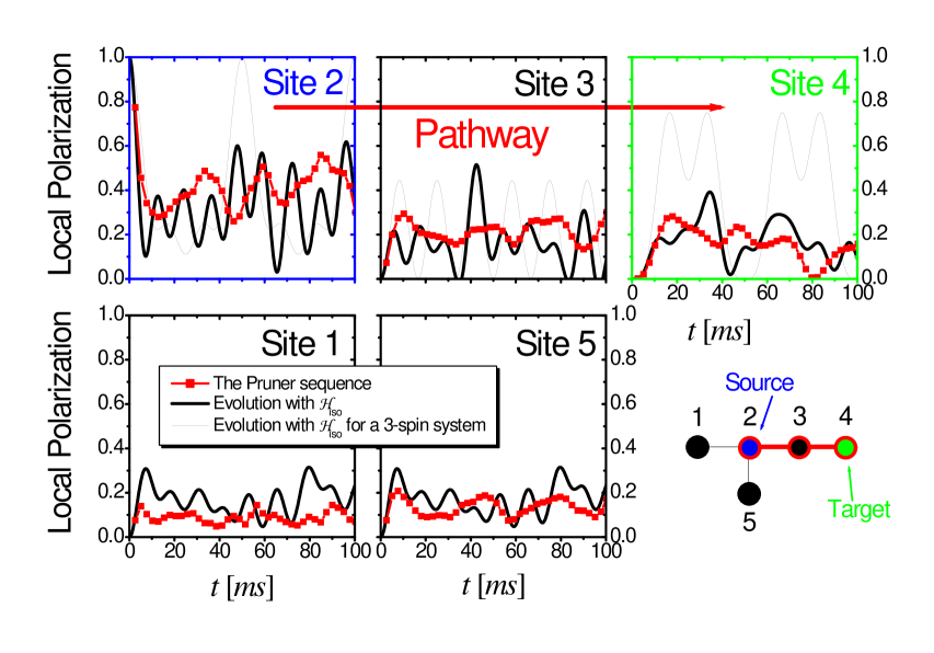
Figure 5.4: Numerical evolution of the local polarization under the pruner sequence at different ¹³C sites in an L-leucine molecule. The ¹³C chemical shifts and nearest neighbor $J$-couplings are given in fig. 5.2. The initial local excitation at site $2$ (the source) is transfered through the selected pathway ($2-3-4$), to site $4$ (the target). The free evolution time is $\Delta t_{\mathrm{free}}=0.27292\operatorname{ms}=2\times\hbar/\Delta_{24}\approx\hbar/\Delta_{23}\approx 2\times\hbar/\Delta_{34}$ and $\Delta t_{\mathrm{iso}}=2.3\operatorname{ms}\approx\frac{1}{11}\frac{\hbar}{J}.$ A gain of $152\%$ relative to the first maximum of the isotropic evolution is observed at site $4.$

one obtains a gain of approximately $152\%$. There, we can observe that the pruning is not working so good as in the previous example. This seems to be a consequence of the fact that carbons $1$ and $5$ do not differ much in chemical shift from carbon $2,$ requiring more cycles of the sequence to dephase appreciably from the selected carbons.

5.2.1 Alternative mixing Hamiltonians

As we mention in section § 5.1, the pruner sequence stroboscopically interrupts the spin-spin interaction to “disconnect” those spins which do not belong to the “selected transfer pathway”. Here, we will show what happens if we change the mixing Hamiltonian. We consider the following mixing Hamiltonians

$$\widehat{\mathcal{H}}_{\mathrm{mix}}^{\mathrm{XY}} =\sum_{i\neq j}J_{ij}\left(\hat{I}_{i}^{y}\hat{I}_{j}^{y}+\hat{I}_{i}^{x}\hat{I}_{j}^{x}\right),$$ (5.7)

$$\widehat{\mathcal{H}}_{\mathrm{mix}}^{\mathrm{dip}} =\sum_{i\neq j}J_{ij}\left(2\hat{I}_{i}^{z}\hat{I}_{j}^{z}-\hat{I}_{i}^{y}\hat{I}_{j}^{y}-\hat{I}_{i}^{x}\hat{I}_{j}^{x}\right),$$ (5.8)

where the first is an XY (planar) Hamiltonian and the second one is a truncated dipolar. We mention in previous chapters that the XY Hamiltonian is less “diffusive”, i.e., the intensities of the coherences are less attenuated. Moreover, an XY dynamics can be solved exactly in some systems [FBE98, FR99, DPL02] as we have done in section § 3.5 to test new theoretical methods. This Hamiltonian is experimentally achievable in liquid [MBSH⁺97] and solid-state [DMF00, CCCR06] NMR while the truncated dipolar Hamiltonian is the natural interaction in solid-state NMR [Abr61, EBW91, Sli92]. We apply these mixing Hamiltonians to the L-leucine molecule to show the main differences in the pruner sequence performance. Note that with the purpose of comparing the effect of the different anisotropies in the mixing Hamiltonian, we have kept the chemical shift and coupling values of the isotropic interaction in the liquid-state. A real solid-state $\widehat{\mathcal{H}}_{\mathrm{mix}}^{\mathrm{dip}}$ would require knowledge of the ¹³C-¹³C dipolar couplings and orientation with respect to the external magnetic field. Figures 5.5 and 5.6 show the polarization dynamics for a source at site $1$ for an XY and a dipolar Hamiltonian respectively.

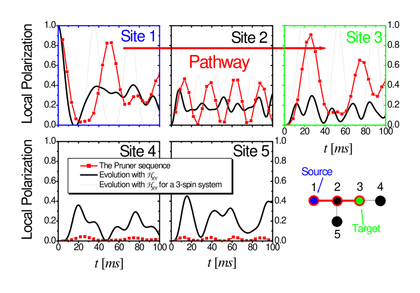
Figure 5.5: Local polarization evolution with the pruner sequence at different ¹³C sites in an L-leucine molecule under an XY mixing Hamiltonian. The initial local excitation at site $1$ (the source) is transfered through the selected pathway ($1-2-3$), to site $3.$ The free evolution time is $\Delta t_{\mathrm{free}}=1.2744\operatorname{ms}=6\times\hbar/\Delta_{13}\approx\hbar/\Delta_{12}\approx 5\times\hbar/\Delta_{23}$ and $\Delta t_{\mathrm{iso}}=3.1\operatorname{ms}\approx\frac{1}{8}\frac{\hbar}{J}.$ A gain of approx. $420\%$ relative to the first maximum of the isotropic evolution is observed at site $3.$

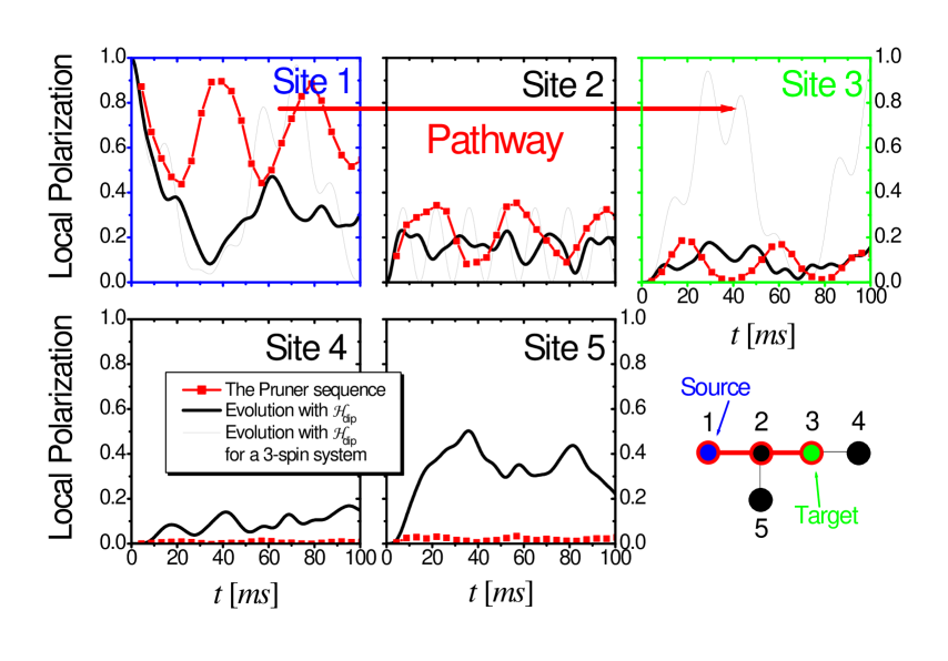
Figure 5.6: Local polarization evolution with the pruner sequence at different ¹³C sites in an L-leucine molecule under a truncated dipolar mixing Hamiltonian. The initial local excitation at site $1$ (the source) is transfered through the selected pathway ($1-2-3$), to site $3.$ The free evolution time is $\Delta t_{\mathrm{free}}=1.2744\operatorname{ms}=6\times\hbar/\Delta_{13}\approx\hbar/\Delta_{12}\approx 5\times\hbar/\Delta_{23}$ and $\Delta t_{\mathrm{iso}}=3.1\operatorname{ms}\approx\frac{1}{8}\frac{\hbar}{J}.$ A gain of approx. $234\%$ relative to the first maximum of the isotropic evolution is observed at site $3.$

The pruner sequence (red lines) is optimized to transfer polarization to the site $3$ (the target) through site $2.$ It is noticeable the performance of our sequence under the XY Hamiltonian. It almost reproduces the isolated three-spin system dynamics (gray lines). The Ising term of the mixing Hamiltonian originates the decrease of the performance in the other Hamiltonians because it produces an effective energy difference between the sites of the pathway. This detuning does not allow for very high polarization transfers. This can be seen in the polarization dynamics of site $1,$ where for the XY mixing (fig. 5.5) the polarization transfer is almost complete, whereas in the dipolar (fig. 5.6) and isotropic (fig. 5.3) cases, only around half of the polarization is transferred. In spite of this, if the goal is the efficiency of the pruning and not the amount of polarization transfer, the pruner sequence works quite well even for isotropic or dipolar interactions.

5.2.2 Step by step pruning of the branches

We have shown how to “isolate” a selected group of spins. Now, we will show the suitability of this technique to choose a first group of spins during a time interval and then to select another group to transfer the polarization from the previous one. In order to do this, firstly, we optimize the pruner sequence to transfer the polarization from site $1$ to site $2$. Then, once the polarization arrived at site $2$, we optimize the sequence to transfer the magnetization to site $3.$ Fig. 5.7 shows this step by step pruning for different mixing Hamiltonians.

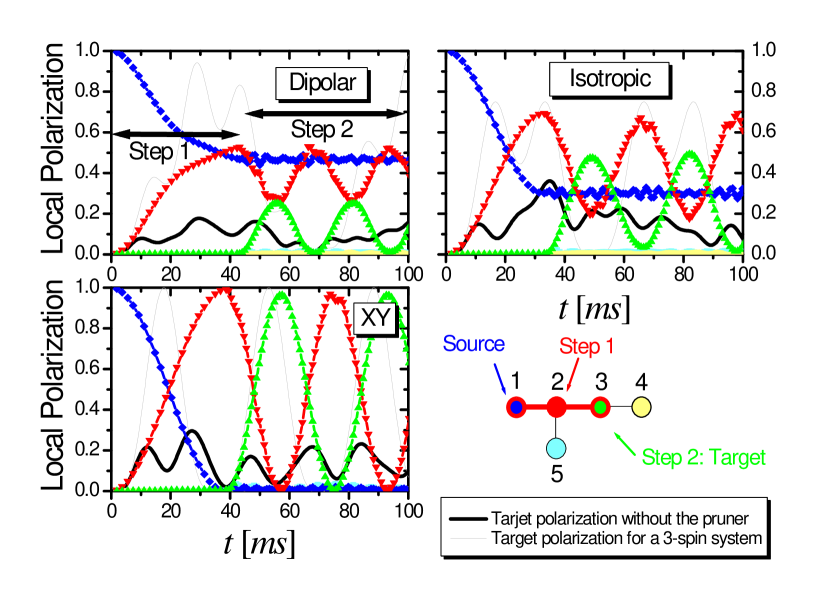
Figure 5.7: Local polarization evolution at different ¹³C sites in an L-leucine molecule under a step by step version of the pruner sequence for XY, isotropic and dipolar mixing Hamiltonians. The scattered lines show the polarization evolution with this pruner sequence, whereas the solid lines show the evolution under the mixing Hamiltonian for the five spins (black) and a three-spin chain (gray). The initial local excitation at site $1$ (the source) is transfered to site $2$ in the first step of the sequence. Within this step the free evolution time is $\Delta t_{\mathrm{free}}=1.2422\operatorname{ms}=\hbar/\Delta_{12}$ and $\Delta t_{\mathrm{iso}}=0.6\operatorname{ms}\ll\frac{\hbar}{J}.$ Within the second part of the sequence, the free evolution time $\Delta t_{\mathrm{free}}=0.2562\operatorname{ms}=\hbar/\Delta_{23}$ optimizes the polarization transfer between sites $2$ and $3$ once the polarization arrived at site $2.$

We observe only the interaction between site $1$ (blue line) and site $2$ (red line) during the the first step of the sequence where $\Delta t_{\mathrm{free}}^{(1\text{{-step}})}=2\pi\hbar/\left|\Delta_{12}\right|.$ It is very similar to the isolated two-spin polarization evolution until these spins are disconnected in the second step of the sequence by keeping only the interaction between sites $2$ and $3$. Within this step, we use $\Delta t_{\mathrm{free}}^{(2\text{{-step}})}=2\pi\hbar/\left|\Delta_{23}\right|$ to optimize the transfer between sites $2$ and $3.$ Thus, in the figures, one can observe the two-spin dynamics between the sites $2$ and $3$ while the others remain frozen. The figures show essentially a pure two-spin polarization evolution. This resembles the quantum Zeno phase predicted in chapter 4 for the swapping operation [ÁDLP06, DÁLP07] which arises when the system-environment interaction is much stronger than the system interaction. There, the Ising system-environment interaction, in the stroboscopic version [ÁDLP06, ÁDLP07a], acted as a measurement process freezing the quantum oscillations. Moreover, the manifestation of this phase in a three-spin system leads to “isolate” the two spins not directly connected to the environment [ÁLP07]. Here, the pruner sequence has stroboscopic free evolutions that act as an environment producing an effective Ising system-environment interaction over the “non-selected” spins, isolating the selected ones. This resembles the applications of engineered reservoir techniques for fundamental studies of decoherence [MKT⁺00, Paz01].

5.3 Summary

We developed a new NMR pulse sequence, “the pruner”, to improve the transfer of polarization through a specific pathway in a system of many interacting spins [ÁDL⁺07]. The sequence effectively prunes branches of spins, where no polarization is required, during the polarization transfer procedure. We obtained a remarkable enhancement, higher than $200\%$, of the polarization transfer with respect to the standard methods. Moreover, by changing the mixing Hamiltonian to an XY interaction, we obtain a gain of about $400\%$. Therefore, it is a very practical tool for NMR applications where a signal gain is of great importance. However, from a fundamental point of view, it is the starting point of an engineered application of the stroboscopic model [ÁDLP06, ÁDLP07a] described in section § 3.3 which seems to manifest a spin dynamics within the quantum Zeno phase [ÁDLP06, DÁLP07]. Moreover, it can help to go deeper in the understanding of decoherence processes and consequently of the environmentally induced quantum dynamical phase transition [ÁDLP06, DÁLP07].

Chapter 6 Entanglement as a tool for ensemble spin dynamics calculations

The quantum time evolution of a qubit cluster of intermediate size is of great interest because its potential applications to quantum information processing (QIP) [Kan98, BD00], and structural characterization through Nuclear Magnetic Resonance [PLU95, MBSH⁺97, CÁL⁺03, RSB⁺05]. Experimental realizations and control of a pure-state dynamics is still one of the major challenges in nowadays quantum physics [QCR04]. Therefore, one generally has to deal with ensemble evolutions, as done in previous chapters for the study of NMR spin dynamics and in related works [PLU95, MBSH⁺97, RSB⁺05]. There, the dynamics is from an initial mixed-state that, as discussed in the Introduction, gives rise to the development of the ensemble quantum computation [VSC04, SSB05]. Hence, it is necessary to find a way to calculate or simulate the ensemble evolution efficiently. Theoretical solutions of the ensemble dynamics arise from the integration of the Liouville von-Neumann equation (see chapter 2) or alternative methods like the Keldysh formalism, discussed in chapter 3 which, for some special cases, yield exact analytical results [DFL02, DPÁ05]. However, in the most general situations, one has to resort to numerical solutions. There are different numerical methods to solve the time dependent evolution, such as exact diagonalization, the Suzuki-Trotter Product-Formula (STPF) and the Chevyshev Polynomial among others [RM04]. These methods are limited by the exponential growth of the Hilbert space dimension with the system size [RM04]. The STPF allows one to treat systems of greater dimension than the exact diagonalization method which is presently limited to around $20$ qubits. The use of the STPF to obtain the dynamics of a pure initial state avoids the storage of the Hamiltonian matrix to be diagonalized. The computation of an ensemble dynamics with an initial mixed-state, requires the calculation of the individual evolutions of each of its components. These are of the order of the Hilbert space dimension demanding long computational times. Here, in order to overcome this limitation, we take profit of the quantum parallelism [SKL02] to calculate the ensemble dynamics through a pure entangled state evolution using the STPF. Apparently, the underlying physical mechanism that makes possible these efficient simulations is the rapid intrinsic decoherence of highly correlated many-qubit systems [KS04, KS06, CCCR06, SPL07].

We consider a system of $M$ spins $1/2$ to calculate the $M$-qubits dynamics. We compare the time evolution of a local polarization (experimentally observed by NMR) [ZME92b, LUP98], between an initial ensemble of local excitations and an initial pure entangled state. This entangled state is built in as a superposition of each of the ensemble components where the complex coefficients of the linear combination are the thermal weights with random phases. We show that the contribution of the coherences of the pure initial state to the dynamics can be neglected due to a self averaging property arising on the destructive interference of the random phases. To show the relevance of the number of independent phases, which are of the order of the Hilbert space dimension, we also calculate the same evolution with an initial pure product state where the number of independent phases are of the order of the system size. We compare the entangled state and ensemble calculations in two contrasting topological configurations: one with relevant mesoscopic effects and other where the disorder makes these effects negligible.

6.1 Ensemble vs. pure entangled state evolution

Let us start considering a system of $M$ spins $1/2$. As we are interested in the evolution of a local excitation, we take the ensemble of all states $\left|\Psi_{i}\right\rangle$ representing the many-spin states in the product base along the quantization axis ($z$), with the $n$-th site polarized (spin up). Each of these states has a thermal weight $w_{i}$. The local spin dynamics through this ensemble can be obtained by calculating a generalization of the auto-correlation function $P_{n,n}^{\mathrm{ens}}(t)$ [PLU95]

$$P_{nn}^{\mathrm{ens}}(t)=2\left[{\displaystyle\sum\limits_{i=1}^{2^{M-1}}}{\displaystyle\sum\limits_{f=1}^{2^{M-1}}}w_{i}\left|\left\langle\Psi_{f}\right|e^{-\mathrm{i}\widehat{\mathcal{H}}t/\hbar}\left|\Psi_{i}\right\rangle\right|^{2}-\frac{1}{2}\right].$$ (6.1)

The quantity $\left|\left\langle\Psi_{f}\right|e^{-\mathrm{i}\widehat{\mathcal{H}}t}\left|\Psi_{i}\right\rangle\right|^{2}$represents the probability of finding the $n$-th site polarized in the state $\left|\Psi_{f}\right\rangle$ at time $t$ provided that the same site was polarized at $t=0$ in the state $\left|\Psi_{i}\right\rangle$. The sum over all possible initial and final states $\left|\Psi_{i}\right\rangle$ and $\left|\Psi_{f}\right\rangle$, gives the amount of the $z$ component of the local polarization at time $t$ on the $n$-th site. As the value of the polarization runs from $-1$ to $1$, the eq. (6.1) is properly renormalized. It represents the standard thermal mixture calculation obtained with the density matrix [MBSH⁺97] (see section § 2)

$$P_{nn}^{\mathrm{ens,DM}}\left(t\right)=\frac{\mathrm{Tr}\left\{\hat{I}_{n}^{z}\hat{\sigma}\left(t\right)\right\}}{\mathrm{Tr}\left\{\hat{I}_{n}^{z}\hat{\sigma}\left(0\right)\right\}},$$ (6.2)

where

$$\hat{\sigma}(t) =\hat{U}(t)\hat{\sigma}(0)\hat{U}^{-1}(t),$$ (6.3)

$$\hat{\sigma}\left(0\right) =\frac{\hat{1}+\beta_{\mathrm{B}}\hbar\Omega_{0,I}\hat{I}_{n}^{z}}{\mathrm{Tr}\left\{\hat{1}\right\}}$$ (6.4)

with

$$\hat{U}\left(t\right)=e^{-\mathrm{i}\widehat{\mathcal{H}}t/\hbar}.$$ (6.5)

Within the Keldysh formalism, using equations (3.103) and (3.106), we obtain

$$P_{nn}^{\mathrm{ens,K}}(t)=\frac{\left\langle\Psi_{\mathrm{eq.}}\right|\hat{I}_{n}^{z}(t)\hat{I}_{n}^{z}(0)\left|\Psi_{\mathrm{eq.}}\right\rangle}{\left\langle\Psi_{\mathrm{eq.}}\right|\hat{I}_{n}^{z}(0)\hat{I}_{n}^{z}(0)\left|\Psi_{\mathrm{eq.}}\right\rangle}=\tfrac{2\hbar}{\mathrm{i}}G_{nn}^{<\,}(t,t)-1.$$ (6.6)

The expression (6.1) involves $2^{M-1}$ different dynamics for each of the initial states, see fig. 6.1 a).

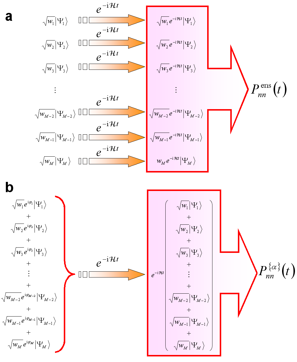
Figure 6.1: Quantum evolution schemes of an ensemble [panel a)] and an entangled pure-state [panel b)]. Each $\left|\Psi_{i}\right\rangle$ represents a simple tensor product state.

This number is directly related to the dimension of the Hilbert space, and thus the number of required evolutions increases exponentially with $M$, leading to large computational times. Our goal is to extract essentially the same information hidden in this ensemble calculation but at a lower cost. To do this we exploit the parallel behavior of quantum systems [SKL02]. This is achieved by replacing the ensemble by only one pure-state, see fig. 6.1 b), obtained as a linear combination of the components of the ensemble, that is,

$$P_{nn}^{\{\alpha\}}(t) =2\left[{\displaystyle\sum\limits_{f=1}^{2^{M-1}}}\left|\left\langle\Psi_{f}\right|e^{-\mathrm{i}\widehat{\mathcal{H}}t/\hbar}\left|\Psi_{\mathrm{pure}}^{\{\alpha\}}\right\rangle\right|^{2}-\frac{1}{2}\right]$$ (6.7)

$$=2\left[{\displaystyle\sum\limits_{f=1}^{2^{M-1}}}\left|\left\langle\Psi_{f}\right|e^{-\mathrm{i}\widehat{\mathcal{H}}t/\hbar}{\displaystyle\sum\limits_{i=1}^{2^{M-1}}}\alpha_{i}\left|\Psi_{i}\right\rangle\right|^{2}-\frac{1}{2}\right].$$ (6.8)

Here $\{\alpha\}$ denotes the set of all the $\alpha_{i}=\sqrt{w_{i}}e^{\mathrm{i}\varphi_{i}}$, with $\varphi_{i}$ an arbitrary phase, involved in the initial pure state. Note that the substantial difference between eq. (6.1) and eq. (6.7) is that the sum in the former is outside the square modulus while in the latter is inside.  Rewriting eq. (6.7), it becomes

$$P_{nn}^{\{\alpha\}}(t)=2\left[{\displaystyle\sum\limits_{f,i=1}^{2^{M-1}}}w_{i}\left|\left\langle\Psi_{f}\right|e^{-\mathrm{i}\widehat{\mathcal{H}}t/\hbar}\left|\Psi_{i}\right\rangle\right|^{2}-\frac{1}{2}\right]\\ +2{\displaystyle\sum\limits_{\genfrac{}{}{0.0pt}{}{f,i,j=1}{i\neq j}}^{2^{M-1}}}\alpha_{i}\alpha_{j}^{\ast}\left\langle\Psi_{f}\right|e^{-\mathrm{i}\widehat{\mathcal{H}}t/\hbar}\left|\Psi_{i}\right\rangle\left\langle\Psi_{j}\right|e^{\mathrm{i}\widehat{\mathcal{H}}t/\hbar}\left|\Psi_{f}\right\rangle\\ =P_{nn}^{\mathrm{ens}}(t)+2{\displaystyle\sum\limits_{\genfrac{}{}{0.0pt}{}{f,i,j=1}{i\neq j}}^{2^{M-1}}}\alpha_{i}\alpha_{j}^{\ast}\left\langle\Psi_{f}\right|e^{-\mathrm{i}\widehat{\mathcal{H}}t/\hbar}\left|\Psi_{i}\right\rangle\left\langle\Psi_{j}\right|e^{\mathrm{i}\widehat{\mathcal{H}}t/\hbar}\left|\Psi_{f}\right\rangle,$$ (6.9)

where we can see that the cross terms make the difference between $P_{nn}^{\mathrm{ens}}(t)$ and $P_{nn}^{\{\alpha\}}(t).$ It is evident that the choice of the phases $\varphi_{i}$ has a relevant role in the equivalence between eq. (6.7) and eq. (6.1). For $M\rightarrow\infty$ and choosing the $\varphi_{i}$ randomly distributed, where $\left|\Psi_{\mathrm{pure}}^{\{\alpha\}}\right\rangle$ is an entangled state, we observe that the cross terms in eq. (6.9) average to zero and

$$P_{nn}^{\mathrm{ens}}(t)=P_{nn}^{\{\alpha\}}(t).$$ (6.10)

This self averaging property of a randomly correlated pure-state, assisted by the large dimension of the Hilbert space, suggests an “intrinsic decoherence” characteristic of very complex systems. As we are considering the whole system, one does not expect to observe decoherence as defined in chapter 1. Nevertheless, the observable involves a single spin of the system and consequently we cannot distinguish between a mixed-state and a pure entangled one, which effectively reflects a loss of information. However, for finite size systems, this self averaging property depends on their particular characteristics as shown below. When the self averaging property is not satisfied, an extra average over initial states is mandatory to force the equality between $P_{nn}^{\mathrm{ens}}(t)$ and $P_{nn}^{\{\alpha\}}(t)$. Then,

$$P_{nn}^{N_{\alpha}}(t)=\frac{1}{N_{\alpha}}{\displaystyle\sum\limits_{\{\alpha\}}^{N_{\alpha}}}P_{nn}^{\{\alpha\}}(t),$$ (6.11)

where $N_{\alpha}$ denotes the number of different realizations of the sets $\{\alpha\}$. One has to perform $N_{\alpha}$ evolutions in the last expression, while for an ensemble dynamics one needs $2^{M-1}$. Thus, the calculation time is reduced by a factor of $N_{\alpha}/2^{M-1}$ where, for an appropriate choice of the $\{\alpha\}$ coefficients, $N_{\alpha}$ $\ll 2^{M-1}$.

6.2 Application to spin-systems with different coupling networks

6.2.1 The systems

In typical situations of high-field solid-state NMR [Abr61, EBW91], the spin interaction Hamiltonian $\widehat{\mathcal{H}}$ can be expressed by eq. (4.3). One can effectively eliminate the Zeeman contribution by working on-resonance in the rotating frame [Sli92]. Then, we can focus in the spin-spin interaction,

$$\widehat{\mathcal{H}}={\textstyle\sum\limits_{i<j}^{M}}\left[a_{ij}\hat{I}_{i}^{z}\hat{I}_{j}^{z}+\tfrac{1}{2}b_{ij}\left(\hat{I}_{i}^{+}\hat{I}_{j}^{-}+\hat{I}_{i}^{-}\hat{I}_{j}^{+}\right)\right],$$

where, $b_{ij}/a_{ij}=0$ represents an Ising-like coupling, $a_{ij}/b_{ij}=0$ an $XY$ Hamiltonian, $a_{ij}/b_{ij}=1$ the isotropic one, and $a_{ij}/b_{ij}=-2$ a dipolar (secular) Hamiltonian truncated with respect to a Zeeman field along the $z$ axis.

In order to show the potential of the proposal summarized in eq. (6.11), we will apply it to two different spin systems which have well differentiated kinds of dynamics:

a) A ladder of spins interacting through an XY Hamiltonian, as shown in fig. 6.3 a). There, $a_{ij}=0,$ $b_{i,i+1}=b_{i+M/2,i+M/2+1}=b_{x}$ and $b_{i,i+M/2}=b_{y}$. Here, the dynamics presents long lived recurrences, showed in the black line of fig. 6.3, due to the ordered topology [PLU95, MBSH⁺97].

b) A star system in which all the spins are interacting with each other through a dipolar coupling, $a_{ij}/b_{ij}=-2,$ with a Gaussian random distribution with zero mean and $\sigma^{2}$ variance for the intensities of the couplings [see fig. 6.3 b)]. In this case, the local polarization decays with a rate proportional to the square root of the local second moment of the Hamiltonian and no recurrences are observed. The black line of fig. 6.4 shows the local polarization of this system.

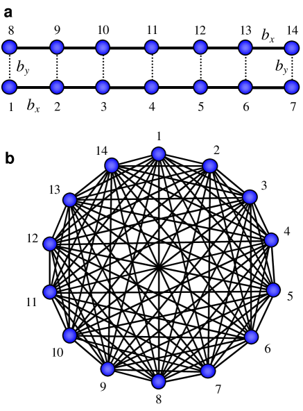
Figure 6.2: Panel a) shows a ladder of spins interacting through an $XY$ Hamiltonian where the horizontal couplings are given by $b_{x}$ and the vertical by $b_{y}.$ Panel b) contains a star system in which all the spins interact with each other through a dipolar coupling, $a_{ij}/b_{ij}=-2,$ with gaussian random distribution with zero mean and $\sigma^{2}$ variance.

In order to compare eqs. (6.1) and (6.11), and the dependence of eq. (6.11) on the choice of the phases $\varphi_{i}$, we calculate the evolution for two types of initial states in the infinite temperature limit, i.e. $w_{i}=1/2^{M-1}$. This limit corresponds to the NMR experimental condition [Abr61]. The particular initial conditions are states with a local excitation on the $n$-th site over a background level which is determined by the zero magnetization of the others $M-1$ spins. These states are used in several NMR experiments [ZME92b, PLU95, MBSH⁺97].

The pure entangled state has the phases $\varphi_{i}$ randomly chosen and $\left|\Psi_{\mathrm{pure}}^{\{\alpha\}}\right\rangle$ becomes

$$\left|\Psi_{\mathrm{ent}}^{\{\alpha\}}\right\rangle={\textstyle\sum_{i=1}^{2^{M-1}}}\tfrac{1}{\sqrt{2^{M-1}}}e^{-\mathrm{i}\varphi_{i}}\left|\Psi_{i}\right\rangle.$$ (6.12)

The correlation function, eq. (6.11), calculated with this state will be called $P_{nn}^{\mathrm{ent},N_{\alpha}}(t).$

The second case is a product (unentangled) state, built with the $n$-th spin up and all the others in a linear combination of spins up and down, with equal probability and randomly correlated. Assuming $n=1$, we have

$$\left|\Psi_{\mathrm{prod}}^{\{\alpha\}}\right\rangle=\left|\uparrow\right\rangle_{1}{\textstyle\bigotimes}\prod\limits_{m=2}^{M}\left|\rightarrow\right\rangle_{m},$$ (6.13)

where

$$\left|\rightarrow\right\rangle_{m}=\tfrac{1}{\sqrt{2}}\left(\left|\downarrow\right\rangle+\left|\uparrow\right\rangle e^{-\mathrm{i}\varphi_{m}}\right).$$

Note that this state is a particular case of (6.12) with a special correlation on the phases $\varphi_{i}$. Here, the correlation function (6.11) will be identified as $P_{nn}^{\mathrm{prod},N_{\alpha}}(t)$.

6.2.2 Quantum evolution

The local polarization, $P_{11}^{\mathrm{ens}}(t),$ obtained with eq. (6.1), for the ladder system composed of $14$ spins is shown in fig. 6.3 with black line.

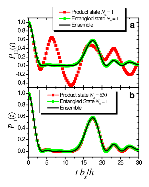
Figure 6.3: Polarization evolution of the local spin dynamics in a $14$-spin ladder system of an ensemble compared with an entangled pure-state dynamics. The ratio between the $x$ and $y$ coupling in the ladder is given by $b_{y}/b_{x}=1/10.$ The black line shows the ensemble local polarization, $P_{11}^{\mathrm{ens}}(t),$ and the red and green lines correspond to the evolution obtained with $P_{11}^{\mathrm{prod},N_{\alpha}}(t)$ and $P_{11}^{\mathrm{ent},N_{\alpha}}(t)$ respectively. The upper panel shows the dynamics of eq. (6.11) for $N_{\alpha}=1$. The lower panel shows the dynamics for $P_{11}^{\mathrm{prod},N_{\alpha}}(t)$ and $P_{11}^{\mathrm{ent},N_{\alpha}}(t)$, where $N_{\alpha}$ is the lower value for which each curve reproduces the ensemble dynamics.

Red and green lines correspond to the temporal evolution of eq. (6.11), $P_{11}^{\mathrm{prod},N_{\alpha}}(t)$ and $P_{11}^{\mathrm{ent},N_{\alpha}}(t)$ respectively. The upper panel shows the dynamics of eq. (6.11) for $N_{\alpha}=1$. The agreement between $P_{11}^{\mathrm{ens}}(t)$ and $P_{11}^{\mathrm{ent},1}(t)$ is excellent, while $P_{11}^{\mathrm{prod},1}(t)$ has a dynamics far away from that of the ensemble. The difference between the dynamics of the two initial pure states is due to the different number of independent random phases (uncorrelated phases) of each state. In the entangled state, there are $2^{M-1}$ independent random phases that make possible the cancellation of the second term in the rhs of eq. (6.9). However, the number of independent phases for the product state is $M-1$. This implies that there are multiple correlations between the phases in the cross terms impeding their self cancellation for low values of $M$.

The lower panel in fig. 6.3 shows the dynamics for $P_{11}^{\mathrm{prod},N_{\alpha}}(t)$ and $P_{11}^{\mathrm{ent},N_{\alpha}}(t)$, where $N_{\alpha}$ is the lower value for which each curve reproduces the ensemble dynamics. Note that the relation between $N_{\mathrm{prod}}$ and $N_{\mathrm{ent}}$ comes from the equivalence in the number of independent phases

$$N_{\mathrm{ent}}2^{M-1}\simeq N_{\mathrm{prod}}(M-1).$$ (6.14)

This equation for the particular case of fig. 6.3 a) is

$$8192=N_{\mathrm{ent}}2^{M-1}\simeq N_{\mathrm{prod}}(M-1)=7969.$$ (6.15)

The statistical theory of the density matrix [Blu81] is based in the random correlation nature of a real system to describe it as an ensemble state in the thermodynamic limit. Here, we observe that even for small numbers like $14,$ the equivalence between a randomly correlated pure state with an ensemble state remains as a consequence of the dimension of the Hilbert space which grows exponentially with $M.$

In fig. 6.4

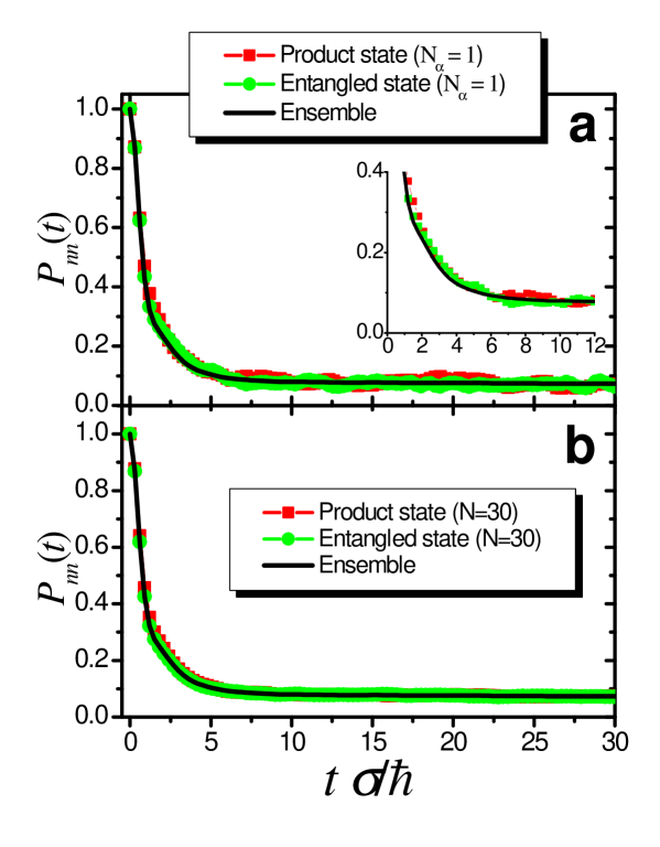
Figure 6.4: Polarization evolution of the local spin dynamics in a star system of $14$ spins. The ensemble dynamics compared with an entangled pure-state evolution is showed. The dipolar interaction $a_{ij}/b_{ij}=-2$ is given by a random normal distribution with zero mean and $\sigma$ variance. The black line shows the ensemble local polarization, $P_{nn}^{\mathrm{ens}}(t),$ and the red and green lines correspond to the evolution obtained with $P_{nn}^{\mathrm{prod},N_{\alpha}}(t)$ and $P_{nn}^{\mathrm{ent},N_{\alpha}}(t)$ respectively. Panel a) shows the dynamics of eq. (6.11) for $N_{\alpha}=1$ and panel b) the dynamics for $P_{nn}^{\mathrm{prod},N_{\alpha}}(t)$ and $P_{nn}^{\mathrm{ent},N_{\alpha}}(t)$, where $N_{\alpha}$ is the lower value for which each curve reproduces the ensemble dynamics.

it is shown the same calculations observed in fig. 6.3 but for a star system. This system shows a spin “diffusion” behavior for the polarization due to the topological complexity yielding the lack of recurrences for long times. For $N_{\alpha}=1$, the upper panel of fig. 6.4 shows that the agreement between the ensemble dynamics and both $P_{nn}^{\mathrm{prod},1}(t)$ and $P_{nn}^{\mathrm{ent},1}(t)$ curves is good only for values of the polarization higher than $0.2$. For times where $P_{nn}^{\mathrm{ens}}(t)$ is close to zero, the cross terms in eq. (6.9) become relevant and both $P_{nn}^{\mathrm{prod},1}(t)$ and $P_{nn}^{\mathrm{ent},1}(t)$ are different from the ensemble curve. Note that in contrast with the ladder case, in this case, the evolutions $P_{nn}^{\mathrm{prod},1}(t)$ and $P_{nn}^{\mathrm{ent},1}(t)$ are similar. For higher values of $N_{\alpha}$ one obtains a better agreement as in the ladder system. It is important to note that the difference between $P_{nn}^{\mathrm{ens}}(t)$, $P_{nn}^{\mathrm{prod},N_{\alpha}}(t)$ and $P_{nn}^{\mathrm{ent},N_{\alpha}}(t)$ would not be appreciable in a real experiment with a typical signal to noise relation.

The ensemble calculation of eq. (6.1) needs to project the evolution of every $2^{M-1}$ initial states, $2^{13}=8192$ for this $14$-spin system, into the same number of possible final states. Instead of this, if one starts with an entangled state or with a random product state, the number of initial states gets significantly reduced. Even for the worst case in which one needs to do $N_{\alpha}\sim 630$ averages to obtain a good agreement with the ensemble curve (low panel of fig. 6.3), this number represents a small fraction, lower than $8\%,$ of the $2^{13}$ initial states of the ensemble. For the case where only one pure entangled state is enough to mimic the ensemble dynamics, the number of evolutions is reduced to a number around the $0.01\%$ of the $2^{13}$ of the ensemble. This shows the potentiality of the method.

6.3 Summary

In summary, in order to overcome the limitations of the numerical calculations of an ensemble spin dynamics when one increases the number of spins, we develop a novel numerical method [ÁDLP07b]. It exploits the delicate property of the quantum superpositions and quantum parallelisms [SKL02] to reproduce the ensemble dynamics through a pure entangled state evolution. The method is useful to use the Suzuki-Trotter product-formula in an ensemble evolution. We showed that the contribution of the coherences of the pure initial state to the dynamics can be neglected due to a self averaging property arising on the destructive interferences of the randomly correlated pure-state. The underlying physical mechanism that makes possible these efficient simulations seems to be related to the observation that higher order coherences in highly correlated states decay faster than those of lower order [KS04, KS06, CCCR06, SPL07]. This suggests that the self averaging property assisted by the large dimension of the Hilbert space could be involved in what is called “intrinsic decoherence”. The concept developed here can be used in two-ways: on one side, it allows for very efficient dynamical calculations of common experimental situations where big ensembles are involved. On the other side, it sheds light on how to experimentally prepare entangled states for specific purposes.

Chapter 7 Conclusion and final remarks

In this thesis we had a dive into quantum dynamics focused in the decoherence phenomenon. Usually, one wants to manipulate a particular system but inevitably other degrees of freedom interact with it changing its dynamics. In order to continue using the potentialities of the system of interest, this led us to study how these external degrees of freedom disturb the system dynamics While this work was done within the NMR field, the workhorse of quantum mechanics, our results could be applicable to many fields because they involve fundamental concepts of quantum mechanics.

In the beginning, we studied the cross-polarization technique for molecular characterization purposes. Through the well known methodology of the generalized Liouville-von Neumann quantum master equation, typically used in the NMR field, we incorporated the degrees of freedom of the environment. This mechanism was described in chapter 2 where we solved the spin dynamics of many-spin systems. Interested in the $8$CB characterization, we interpreted cross-polarization experiments over this liquid crystal in several mesophases [CÁL⁺03]. The $8$CB molecule, as we described in section § 2.2, could be represented by a three-spin system coupled with a spin-environment. Thus, we began with a simple system to understand the cross-polarization dynamics. Based on the Müller, et al. model [MKBE74], we solved the two-spin dynamics interacting with a fast fluctuating spin-bath. We reobtained their solution and then we extended the model to a three-spin system interacting with a spin-bath. As this molecule has two possible configurations for the heteronuclear coupling, this led us to note that in each space of $M=\pm 1/2$ there are only two of the three eigenstates that are involved in the dipolar transitions that give rise to the oscillations. This was explained as a consequence of the symmetry of the system, i.e. the flip-flop can occur only between the carbon and one (the symmetric or the antisymmetric) combination of the proton states depending on the relative signs of the heteronuclear couplings ($b_{1}=b_{2}$ or $b_{1}=-b_{2}$) [CÁL⁺03]. Hence, the frequency of the oscillation depends of the different configurations. The experimental data were well fitted to the analytical polarization expression concerning the oscillation frequency. However, the relaxation process was not well described using a direct extension of the MKBE model with an isotropic system-environment interaction. This was manifested by the fact that the experimental cross-polarization data of the $8$CB molecule showed that the rate of attenuation of the oscillations is much faster than the rate of polarization transfer from the bath. Consequently, we extended the MKBE model to obtain a relaxation superoperator that takes into account this phenomenon arising from an anisotropic system-environment interaction [CÁL⁺03, ÁLP07]. The anisotropy is given by the ratio between the interaction rates of the Ising and XY term. We emphasized the different roles of the anisotropy of the system-environment interaction on decoherence and relaxation processes. The main difference is that while the XY interaction takes the system to the total system equilibrium, the Ising system-environment interaction takes it to an internal quasi-equilibrium [CÁL⁺03, ÁLP07]. The introduced anisotropy could be explained in the nematic phase by assuming a dipolar system-environment interaction Hamiltonian within the extreme narrowing approximation. Nevertheless, in the smectic phase the anisotropy is much more pronounced. Hence, we extended the model outside the fast fluctuation approximation to take into account slower motions. In this way, a better agreement with the experimental observations was obtained without resorting to other mechanisms which operate in both phases [CÁL⁺03]. This detailed spin dynamics calculations allowed us to obtain separately the homonuclear and heteronuclear dipolar couplings in CH₂ systems which constitute the $8$CB molecule [CÁL⁺03]. We tested the reliability of the results with an experimental direct determination of the heteronuclear couplings using cross-polarization under Lee-Goldburg conditions.

Within a fundamental point of view, we observed that the solutions based on the MKBE model did not describe the quantum quadratic short time behavior nor the features displayed in fig. 1.6 within the $b\ll\Gamma_{\mathrm{SE}}$ region. In order to overcome these limitations, a further improvement was done including non-secular terms of the system-environment interaction to extend the solution. This solution describes well the experimental short time behavior and led us, together with the spin dynamics analysis within the Keldysh formalism (chapter 3), to enrich our perspectives.

Inspired in the generalized Landauer-Büttiker equation within the Keldysh formalism, we obtained that the initially phenomenological stroboscopic model [ÁDLP06], in the continuous form, led to the non-secular solution within the generalized quantum master equation. This induced us to obtain analytical results of the spin dynamics from microscopic derivation and characterization of the system-environment interaction [DPÁ05, DÁLP07, ÁDLP07a]. To do that, we solved the Schrödinger equation within the Keldysh formalism for an open system under the wide band regime in the environment (fast fluctuation approximation). Within this formalism, assisted by the Jordan-Wigner transformation that maps a spin system into a fermion one, an exact solution for an XY linear chain is obtainable. This allowed us not only to include memory effects within the spin-bath [DPÁ05], discussed in section § 3.5, but it enabled us to test approximation methods to solve the more complex systems of section § 3.4. To describe the spin-bath under the fast fluctuation approximation that leads to interactions local in time, we resorted to the Wigner time-energy variables. This allowed us to transform the density function expressed in the Danielewicz integral form into a generalized Landauer-Büttiker equation. By applying this technique to a two-spin system coupled to a spin-bath [ÁDLP06, ÁDLP07a], we improved the results obtained through the secular approximation within the standard density matrix formalism. Further on, we effectively symmetrized the system-environment interactions virtually transforming them into a spatially homogeneous process [ÁDLP07a]. This involved a uniform system-environment interaction rate that leads to a simple non-hermitian propagator while the original multi-exponential decay processes were recovered by an injection density function. This method led us to interpret the phenomenon of decoherence and the system-environment interaction within a special view: The environment as a measurement apparatus [ÁDLP06]. There, the decoherence takes another perspective: The loss of information of the system entity, i.e. how the isolated system dynamics is degraded in a characteristic time given by the fictitious homogeneous decoherence time. The homogenization procedure enabled the microscopic derivation of the stroboscopic model for the system-environment interaction [ÁDLP07a]. While, the stroboscopic process may not be the best description of reality, it provides an optimal numerical algorithm to calculate quantum dynamics in discrete time steps [ÁDLP06, ÁDLP07a].

While the dynamics obtained through the Keldysh formalism are reproduced by the non-secular solution within the generalized quantum master equation, they derive from a microscopic model of the entire system (system plus environment) and the final state must not be hinted beforehand. The Keldysh formalism gives us another perspective to discuss about the physics of the quantum time evolution and the interpretations of the approximations made. For example, the arising of the quantum Zeno effect shown in the decoherence time, $1/\tau_{\phi}\propto\left(b/\hbar\right)^{2}\tau_{\mathrm{SE}}$, could be interpreted as a “nested” Fermi golden rule rate emphasizing the non-perturbative nature of the result [ÁDLP06].

The manifestation of the quantum Zeno effect led us to a novel interpretation of previous experiments [LUP98] shown in fig. 1.6. In chapter 4, we found experimental evidence that environmental interactions can drive a swapping gate (two-spin system) through a Quantum Dynamical Phase Transition towards an over-damped or Zeno phase [ÁDLP06]. The NMR spin swapping experiments in a ¹³C-¹H system enable the identification and characterization of this phase transition as a function of the ratio $b\tau_{\mathrm{SE}}/\hbar$ between the internal and system-environment interaction. The developed microscopic model [DÁLP07, ÁDLP07a] for the swapping operation describes both phases and the critical region with great detail, showing that it depends only on the nature of the interaction [ÁDLP06, ÁDLP07a]. In particular, it shows that the phase transition does not occur if the system-environment interaction gives isotropic interaction rates, $\Gamma_{\mathrm{ZZ}}=\Gamma_{\mathrm{XY}}$. Within the standard approximations typically used to solve the generalized quantum master equation, one tends to think that $\Gamma_{\mathrm{ZZ}}=\Gamma_{\mathrm{XY}}$ corresponds to an isotropic system-environment interaction. However, a careful microscopic derivation within the Keldysh formalism showed us that this is not necessarily correct. It is also important to mention that the spin-bath occupation factor modifies the $\Gamma_{\mathrm{ZZ}}$ rate. For the description of the quantum dynamical phase transition, it is crucial to distinguish between inputs and output parameters. One can visualize applications that range from tailoring the environments for a reduction of their decoherence on a given process to using the observed critical transition in frequency and decoherence rate as a tracer of the environment’s nature. For example, we extended the model to a $3$-spin system to show that beyond a critical region two spins become almost decoupled from the environment oscillating with the bare Rabi frequency and relaxing more slowly [ÁLP07].

Inspired in the stroboscopic model and the arising of the environmentally induced quantum Zeno phase, we developed a new NMR pulse sequence. “The pruner” stroboscopically interrupts the system evolution to improve the transfer of polarization through a specific pathway in a system of many interacting spins [ÁDL⁺07]. The sequence effectively prunes branches of spins, where no polarization is required, during the polarization transfer procedure. We obtained a remarkable enhancement of the polarization transfer with respect to the standard methods. Therefore, it is a very practical tool for NMR applications where a signal gain is of great importance. However, from a fundamental point of view, it is the starting point of an engineered application of the stroboscopic model [ÁDLP06, ÁDLP07a] described in section § 3.3 which seems to manifest a spin dynamics within the quantum Zeno phase [ÁDLP06, DÁLP07]. Moreover, it can help to go deeper in the understanding of decoherence processes and consequently of the environmentally induced quantum dynamical phase transition [ÁDLP06, DÁLP07].

Finally, in order to study the spin dynamics of larger systems, we developed a novel numerical method that exploits quantum parallelism [ÁDLP07b]. This provides a tool to overcome the limitations of standard numerical calculations of ensemble spin dynamics for high number of spins. Hence, this numerical method constitutes the starting point to extend the study of the quantum dynamical phase transition to larger systems and how it is involved in the irreversibility phenomena. Moreover, the observation that the contribution of many coherences of an entangled randomly correlated state to the dynamics can be neglected due to a self averaging property, opens a fundamental question: Is this self averaging property involved in what is called “intrinsic decoherence”?

Bibliography

- [Abr61] A. Abragam, Principles of nuclear magnetism, Oxford University Press, London, 1961.
- [ÁDL+07] G. A. Álvarez, E. P. Danieli, P. R. Levstein, H. M. Pastawski, and L. Frydman, Polarization transfer enhancement by selective pruning of a branched coupling pathway in NMR, In preparation (2007).
- [ÁDLP06] G. A. Álvarez, E. P. Danieli, P. R. Levstein, and H. M. Pastawski, Environmentally induced quantum dynamical phase transition in the spin swapping operation, J. Chem. Phys. 124 (2006), 194507.
- [ÁDLP07a] , Decoherence under many-body system-environment interactions: A stroboscopic approach through a fictitiously homogenized interaction rate, Sent for publication. cond-mat/0701574 (2007).
- [ÁDLP07b] , Entanglement as a tool for ensemble spin dynamics, In preparation (2007).
- [ÁLP07] G. A. Álvarez, P. R. Levstein, and H. M. Pastawski, Signatures of a quantum dynamical phase transition in a three-spin system in presence of a spin environment, To be published in Physica B. cond-mat/0703158 (2007).
- [ALW92] B. L. Altshuler, P. A. Lee, and R. A. Webb, Mesoscopic phenomena, North Holland, Amstermdam, 1992.
- [Ave99] D. V. Averin, Solid-state qubits under control, Nature 398 (1999), 748.
- [BD85] A. Bax and D. G. Davis, MLEV-17-based two-dimensional homonuclear magnetization transfer spectroscopy, J. Magn. Reson. 65 (1985), 355.
- [BD00] C. H. Bennett and D. P. DiVincenzo, Quantum information and computation, Nature 404 (2000), 247.
- [BE83] L. Braunschweiler and R. R. Ernst, Coherence transfer by isotropic mixing: Application to proton correlation spectroscopy, J. Magn. Reson. 53 (1983), 521.
- [BEY+03] N. Boulant, K. Edmonds, J. Yang, M. A. Pravia, and D. G. Cory, Experimental demonstration of an entanglement swapping operation and improved control in NMR quantum-information processing, Phys. Rev. A 68 (2003), 032305.
- [BHP46a] F. Bloch, W. W. Hansen, and M. Packard, Nuclear induction, Phys. Rev 69 (1946), 127.
- [BHP46b] , The nuclear induction experiment, Phys. Rev. 70 (1946), 474.
- [Blo46] F. Bloch, Nuclear induction, Phys. Rev. 70 (1946), 460.
- [Blu81] K. Blum, Density matrix: Theory and applications, Plenum Press, New York, 1981.
- [CÁL+03] A. K. Chattah, G. A. Álvarez, P. R. Levstein, F. M. Cucchietti, H. M. Pastawski, J. Raya, and J. Hirschinger, Many-spin quantum dynamics during cross polarization in 8CB, J. Chem. Phys. 119 (2003), 7943.
- [CCCR06] H. Cho, P. Cappellaro, D. G. Cory, and C. Ramanathan, Decay of highly correlated spin states in a dipolar-coupled solid: NMR study of CaF2, Phys. Rev. B 74 (2006), 224434.
- [CCH+02] A. K. Chattah, F. M. Cucchietti, M. Hologne, J. Raya, and P. R. Levstein, Radiofrequency-induced temperature increase as a function of cross polarization contact time in 8 CB, Mag. Res. Chem. 40 (2002), 772.
- [CEHL85] C. J. R. Counsell, J. W. Emsley, N. J. Heaton, and G.R. Luckurst, Orientational ordering in uniaxial liquid crystals, Mol. Phys. 54 (1985), 847.
- [CHEP96] S. Caldarelli, M. Hong, L. Emsley, and A. Pines, Measurement of carbon-proton dipolar couplings in liquid crystals by local dipolar field NMR spectroscopy, J. Phys. Chem. 100 (48) (1996), 18696.
- [CL83a] A. O. Caldeira and A. J. Leggett, Ann. Phys. (N. Y.) 153 (1983), 445(E).
- [CL83b] , Path integral approach to quantum brownian motion, Physica A 121 (1983), 587.
- [CL83c] , Quantum tunnelling in a dissipative system, Ann. Phys. (N. Y.) 149 (1983), 374.
- [CPH98] D. G. Cory, M. D. Price, and T. F. Havel, Nuclear magnetic resonance spectroscopyan experimentally accessible paradigm for quantum computing, Physica D 120 (1998), 82.
- [CPJ04] F. M. Cucchietti, H. M. Pastawski, and R. A. Jalabert, Universality of the Lyapunov regime for the Loschmidt echo, Phys. Rev. B 70 (2004), 035311.
- [DÁLP07] E. P. Danieli, G. A. Álvarez, P. R. Levstein, and Horacio M. Pastawski, Quantum dynamical phase transition in a system with many-body interactions, Solid State Comm. 141 (2007), 422.
- [Dan84] P. Danielewicz, Quantum theory of nonequilibrium processes, i., Ann. Phys. 152 (1984), 239.
- [Dan06] E. P. Danieli, Formalismo para el diseño y control de interferencias cuánticas en la dinámica de polarización en sistemas de espines nucleares, Ph.D. thesis, Facultad de Matemática, Astronomía y Física, 2006.
- [DCM92] J. Dalibard, Y. Castin, and K. Mølmer, Wave-function approach to dissipative processes in quantum optics, Phys. Rev. Lett. 68 (1992), 580.
- [DFL02] S. I. Doronin, E. B. Fel’dman, and S. Lacelle, Multiple-quantum nuclear magnetic resonance spin dynamics in disordered rigid chains and rings, J. Chem. Phys. 117 (2002), 9646.
- [DMF00] S. I. Doronin, I. I. Maksimov, and E. B. Fel’dman, Multiple-quantum dynamics of one-dimensional nuclear spin systems in solids, J. Exp. Theor. Phys. 91 (2000), 597.
- [Don97] R. Y. Dong, Nuclear magnetic resonance of liquid crystals, Springer, New York, 1997.
- [DP90] J. L. D’Amato and H. M. Pastawski, Conductance of a disordered linear chain including inelastic scattering events, Phys. Rev. B 41 (1990), 7411.
- [DPÁ05] E. P. Danieli, H. M. Pastawski, and G. A. Álvarez, Quantum dynamics under coherent and incoherent effects of a spin bath in the Keldysh formalism: Application to a spin swapping operation, Chem. Phys. Lett. 402 (2005), 88.
- [DPL02] E. P. Danieli, H. M. Pastawski, and P. R. Levstein, Exact spin dynamics of inhomogeneous 1-d systems at high temperature, Physica B 320 (2002), 351.
- [DPL04] , Spin projection chromatography, Chem. Phys. Lett. 384 (2004), 306.
- [DRKH03] V. V. Dobrovitski, H. A. De Raedt, M. I. Katsnelson, and B. N. Harmon, Quantum oscillations without quantum coherence, Phys. Rev. Lett. 90 (2003), 210401.
- [DTW75] D. E. Demco, J. Tegenfeldt, and J. S. Waugh, Dynamics of cross relaxation in nuclear magnetic double resonance, Phys. Rev. B 11 (1975), 4133.
- [EBW91] R. R. Ernst, G. Bodenhausen, and A. Wokaun, Principles of nuclear magnetic resonance in one and two dimensions, Oxford University Press, New York, 1991.
- [EMTP98a] M. Ernst, B. H. Meier, M. Tomasselli, and A. Pines, Time-reversal of cross-polarization in nuclear magnetic resonance, J. Chem. Phys. 108 (1998), 9611.
- [EMTP98b] , Time reversal of cross-polarization in solid-state NMR, Mol. Phys. 95 (1998), 849.
- [EPR35] A. Einstein, B. Podolsky, and N. Rosen, Can quantum-mechanical description of physical reality be considered complete?, Phys. Rev. 47 (1935), 777.
- [FBE98] E. B. Fel’dman, R. Brüschweiler, and R. R. Ernst, From regular to erratic quantum dynamics in long spin 1/2 chains with an XY hamiltonian, Chem. Phys. Lett. 294 (1998), 297–304.
- [FKE00] B. M. Fung, A. K. Khitrin, and K. Ermolaev, An improved broadband decoupling. sequence for liquid crystals and solids, Journ. Magn. Reson. 142 (2000), 97.
- [For90] D. Forster, Hydrodynamic fluctuations, broken symmetry, and correlation functions, Addison-Wesley, 1990.
- [FP02] P. Facchi and S. Pascazio, Quantum Zeno subspaces, Phys. Rev. Lett. 89 (2002), 080401.
- [FP06] E. Rufeil Fiori and H. M. Pastawski, Non-markovian decay beyond the fermi golden rule: Survival collapse of the polarization in spin chains, Chem. Phys. Lett. 420 (2006), 35.
- [FPG+86] B. M. Fung, C. Poon, M. Gangoda, E. L. Enwall, T. A. D. Diep, and C. V. Bui, Nematic and smectic ordering of 4-n-octyl-4’-cyanobiphenyl studied by carbon-13 NMR, Mol. Cryst. Liq. Crist. 141 (1986), 267.
- [FR99] E. B. Fel’dman and M. G. Rudavets, Regular and erratic quantum dynamics in spin 1/2 rings with an XY hamiltonian, Chem. Phys. Lett. 311 (1999), 453.
- [Fur36] W. H. Furry, Note on the quantum-mechanical theory of measurement, Phys. Rev. 49 (1936), 393.
- [FV63] R. P. Feynman and F. L. Vernon Jr., The theory of a general quantum system interacting with a linear dissipative system, Ann. Phys. (N.Y.) 24 (1963), 118.
- [GC97] N. A. Gershenfeld and I. L. Chuang, Bulk spin-resonance quantum computation, Science 275 (1997), 350.
- [GFMB03] S. A. Gurvitz, L. Fedichkin, D. Mozyrsky, and G. P. Berman, Relaxation and the Zeno effect in qubit measurements, Phys. Rev. Lett. 91 (2003), 066801.
- [Hah50a] E. L. Hahn, Nuclear induction due to free Larmor precession, Phys. Rev. 77 (1950), 297.
- [Hah50b] , Spin echoes, Phys. Rev. 4 (1950), 580.
- [HH62] S. R. Hartmann and E. L. Hahn, Nuclear double resonance in the rotating frame, Phys. Rev. 128 (1962), 2042.
- [HH94] J. Hirschinger and M. Hervé, Cross-polarization dynamics and spin diffusion in some aromatic compounds, Solid State Nuclear Magnetic Resonance 3 (1994), 121.
- [HL73] K. Hepp and E. H. Lieb, Phase transition in reservoir driven open systems with applications to lasers and superconductors, Helv. Phys. Acta 46 (1973), 573.
- [HL84] W. Horsthemke and R. Lefever, Noise-induced transitions, Springer, Berlin, 1984.
- [JP01] R. A. Jalabert and H. M. Pastawski, Environment-independent decoherence rate in classically chaotic systems, Phys. Rev. Lett. 86 (2001), 2490.
- [JSB01] Ph. Jacquod, P. G. Silvestrov, and C. W. J. Beenakker, Golden rule decay versus Lyapunov decay of the quantum Loschmidt echo, Phys. Rev. E 64 (2001), 055203(R).
- [JW28] P. Jordan and E. Wigner, über das paulische äquivalenzverbot, Z. Phys. 47 (1928), 631.
- [Kan98] B. E. Kane, A silicon-based nuclear spin quantum computer, Nature 393 (1998), 133.
- [Kel64] L. V. Keldysh, Ionization in the field of a strong electromagnetic wave, ZhETF 47 (1964), 1515. [Sov. Phys.–JETP 20, 1018 (1965)].
- [KLG02] A. V. Khaetskii, D. Loss, and L. Glazman, Electron spin decoherence in quantum dots due to interaction with nuclei, Phys. Rev. Lett. 88 (2002), 186802.
- [KS04] H. G. Krojanski and D. Suter, Scaling of decoherence in wide NMR quantum registers, Phys. Rev. Lett. 93 (2004), 090501.
- [KS06] , Reduced decoherence in large quantum registers, Phys. Rev. Lett. 97 (2006), 150503.
- [KWZ96] P. G. Kwiat, H. Weinfurter, and A. Zeilinger, Quantum seeing in the dark, Sci. Am. November (1996), 72.
- [Lan27] L. D. Landau, The damping problem in wave mechanics, Z. Phys. 45 (1927), 430.
- [LCP+04] P. R. Levstein, A. K. Chattah, H. M. Pastawski, J. Raya, and J. Hirschinger, NMR polarization echoes in a nematic liquid crystal, J. Chem. Phys. 121 (2004), 7313.
- [LHBF99] N. Linden, E. Kupce H. Barjat, and R. Freeman, How to exchange information between two coupled nuclear spins: the universal swap operation, Chem. Phys. Lett. 307 (1999), 198.
- [LPD90] P. R. Levstein, H. M. Pastawski, and J. L. D’Amato, Tuning the through-bond interaction in a two-centre problem, J. Phys.: Condens. Matter 2 (1990), 1781.
- [LSM61] E. H. Lieb, T. Schultz, and D. C. Mattis, Two soluble models of an antiferromagnetic chain, Ann. Phys. 16 (1961), 407.
- [LUP98] P. R. Levstein, G. Usaj, and H. M. Pastawski, Attenuation of polarization echoes in NMR: A test for the emergence of dynamical irreversibility in many-body quantum systems, J. Chem. Phys. 108 (1998), 2718.
- [LY01] Xin-Qi Li and Yi Jing Yan, Electrical transport through individual dna molecules, Appl. Phys. Lett. 79 (2001), 2190.
- [MBE98] Z. L. Mádi, R. Brüschweiller, and R. R. Ernst, One- and two-dimensional ensemble quantum computing in spin Liouville space, J. Chem. Phys. 109 (1998), 10603.
- [MBSH+97] Z. L. Mádi, B. Brutscher, T. Schulte-Herbrüggen, R. Brüschweiler, and R. R. Ernst, Time-resolved observation of spin waves in a linear chain of nuclear spins, Chem. Phys. Lett. 268 (1997), 300.
- [MKBE74] L. Müller, A. Kumar, T. Baumann, and R. R. Ernst, Transient oscillations in NMR cross-polarization experiments in solids, Phys. Rev. Lett. 32 (1974), 1402.
- [MKR94] V. Mujica, M. Kemp, and M. A. Ratner, Electron conduction in molecular wires. II. application to scanning tunneling microscopy, J. Chem. Phys. 101 (1994), 6856.
- [MKT+00] C. J. Myatt, B. E. King, Q. A. Turchette, C. A. Sackett, D. Kielpinski, W. M. Itano, C. Monroe, and D. J. Wineland, Decoherence of quantum superpositions through coupling to engineered reservoirs, Nature 403 (2000), 269.
- [MLL03] F. Meier, J. Levy, and D. Loss, Quantum computing with spin cluster qubits, Phys. Rev. Lett. 90 (2003), 047901.
- [MS77] B. Misra and E. C. G. Sudarshan, The Zeno’s paradox in quantum theory, J. Math. Phys. 18 (1977), 756.
- [MTA+06] J. J. L. Morton, A. M. Tyryshkin, A. Ardavan, S. C. Benjamin, K. Porfyrakis, S. A. Lyon, and G. A. D. Briggs, Bang-bang control of fullerene qubits using ultra-fast phase gates, Nature Phys. 2 (2006), 40.
- [NC00] M. A. Nielsen and I. L. Chuang, Quantum computation and quantum information, Cambridge University Press, Cambridge, 2000.
- [Neu32] J. Von Neumann, Mathematische grundlagen der quantenmechanik, Springer, Berlin, 1932.
- [NPT99] Y. Nakamura, Yu. A. Pashkin, and J. S. Tsai, Coherent control of macroscopic quantum states in a single-cooper-pair box, Nature 398 (1999), 786.
- [Omn92] R. Omnès, Consistent interpretations of quantum mechanics, Rev. Mod. Phys. 64 (1992), 339.
- [Pas91] H. M. Pastawski, Classical and quantum transport from generalized Landauer-Büttiker equation, Phys. Rev. B 44 (1991), 6329.
- [Pas92] , Classical and quantum transport from generalized Landauer-Büttike equations. II. time-dependent resonant tunneling, Phys. Rev. B 46 (1992), 4053.
- [Paz01] J. P. Paz, Protecting the quantum world, Nature 412 (2001), 869.
- [PGIN03] S. Pleutin, H. Grabert, G. L. Ingold, and A. Nitzan, The electrostatic potential profile along a biased molecular wire: A model quantum-mechanical calculation, J. Chem. Phys. 118 (2003), 3756.
- [PJT+05] J. R. Petta, A. C. Johnson, J. M. Taylor, E. A. Laird, A. Yacoby, M. D. Lukin, C. M. Marcus, M. P. Hanson, and A. C. Gossard, Coherent manipulation of coupled electron spins in semiconductor quantum dots, Science 309 (2005), 2180.
- [PLU95] H. M. Pastawski, P. R. Levstein, and G. Usaj, Quamtum dynamical echoes in the spin diffusion in mesoscopic systems, Phys. Rev. Lett. 75 (1995), 4310–4313.
- [PLU+00] H. M. Pastawski, P. R. Levstein, G. Usaj, J. Raya, and J. A. Hirschinger, A nuclear magnetic resonance answer to the Boltzmann-Loschmidt controversy?, Physica A 283 (2000), 166.
- [PN94] S. Pascazio and M. Namiki, Dynamical quantum Zeno effect, Phys. Rev. Lett. 50 (1994), 4582.
- [PPB46] E. M. Purcell, R. V. Pound, and N. Bloembergen, Nuclear magnetic resonance absorption in hydrogen gas, Phys. Rev. 70 (1946), 986.
- [PR96] R. Pratima and K. V. Ramanathan, The application to liquid crystals of transient oscillations in cross polarization experiments, Journ. Magn. Reson. A 118 (1996), 7.
- [PSM+03] M. Poggio, G. M. Steeves, R. C. Myers, Y. Kato, A. C. Gossard, and D. D. Awschalom, Local manipulation of nuclear spin in a semiconductor quantum well, Phys. Rev. Lett. 91 (2003), 207602.
- [PTP46] E. M. Purcell, H. C. Torrey, and R. V. Pound, Resonance absorption by nuclear magnetic moments in a solid, Phys. Rev. 69 (1946), 37.
- [PU98] H. M. Pastawski and G. Usaj, Dimensional crossover in spin diffusion: A manifestation of the quantum Zeno effect, Phys. Rev. B 57 (1998), 5017.
- [PUL96] H. M. Pastawski, G. Usaj, and P. R. Levstein, Quamtum interference phenomena in the local polarization dynamics of mesoscopic system: An NMR observation, Chem. Phys. Lett. 261 (1996), 329–334.
- [PZ99] J. P. Paz and W. H. Zurek, 72nd Les Houches Summer School on “coherent Matter Waves”, July-August (1999).
- [QCR04] A quantum information science and technology roadmap, http://qist.lanl.gov/ (2004).
- [RHGG97] P. Reinheimer, J. Hirschinger, P. Gilard, and N. Goetz, Cross-polarization dynamics and proton dipolar local field measurements in some organic compounds, Mag. Res. Chem. 35 (1997), 757.
- [RM04] H. De Raedt and K. Michielsen, Computational methods for simulating quantum computers, quant-ph/0406210. Handbook of Theoretical and Computational Nanotechnology. Quantum and Molecular Computing, Quantum Simulations (American Scientific Publishers, 2006). (2004).
- [RPW70] W. K. Rhim, A. Pines, and J. S. Waugh, Violation of the spin temperature hypothesis, Phys. Rev. Lett. 25 (1970), 218.
- [RSB+05] C. Ramanathan, S. Sinha, J. Baugh, T. F. Havel, and D. G. Cory, Selective coherence transfers in homonuclear dipolar coupled spin systems, Phys. Rev. A 71 (2005), 020303(R).
- [Sac01] S. Sachdev, Quantum phase transitions, Cambridge U. P., 2001.
- [SB04] T. M. Stace and S. D. Barrett, Continuous quantum measurement: Inelastic tunneling and lack of current oscillations, Phys. Rev. Lett. 92 (2004), 136802.
- [Sch35] E. Schrödinger, Die gegenwärtige situation in der quantenmechanik, Naturwissenschaften 23 (1935), 807; 823; 844. The present situation in quantum mechanics: A translation was originally published in Proceedings of the American Philosophical Society, 124, 323–38. And then appeared as Section I.11 of Part I of Quantum Theory and Measurement (J.A. Wheeler and W.H. Zurek, eds., Princeton university Press, New Jersey 1983). For an online version: http://www.tu–harburg.de/rzt/rzt/it/QM/cat.html.
- [Sch00] W. P. Schleich, Engineering decoherence, Nature 403 (2000), 256.
- [Sch04] M. Schlosshauer, Decoherence, the measurement problem, and interpretations of quantum mechanics, Rev. Mod. Phys. 76 (2004), 1267.
- [SHE98] D. Sakellariou, P. Hodgkinson, and L. Emsley, Quasi equilibria in solid-state NMR, Chem. Phys. Lett. 293 (1998), 110.
- [SKE+01] G. Salis, Y. Kato, K. Ensslin, D. C. Driscoll, A. C. Gossard, and D. D. Awschalom, Electrical control of spin coherence in semiconductor nanostructures, Nature 414 (2001), 619.
- [SKL02] J. Schliemann, A. V. Khaetskii, and D. Loss, Spin decay and quantum parallelism, Phys. Rev. B 66 (2002), 245303.
- [SKSM01] B. Stevenson, A. V. Komolkin, D. Sandström, and A. Maliniak, Structure and molecular ordering extracted from residual dipolar couplings: A molecular dynamics simulation study, J. Chem. Phys. 114 (2001), 2332.
- [Sli92] C. P. Slichter, Principles of magnetic resonance, 2nd ed., Springer-Verlag, 1992.
- [SPL07] C. M. Sánchez, H. M. Pastawski, and P. R. Levstein, Time evolution of multiple quantum coherences in NMR, To be published in Phys. B (2007).
- [SRS96] K. Schmidt-Rohr and H. W. Spiess, Multidimensional solid state NMR and polymers, Academic Press, 1996.
- [SSB05] R. Stadelhofer, D. Suter, and W. Banzhaf, Quantum and classical parallelism in parity algorithms for ensemble quantum computers, Phys. Rev. A 71 (2005), 032345.
- [TED+05] J. M. Taylor, H.-A. Engel, W. Dür, A. Yacoby, C. M. Marcus, P. Zoller, and M. D. Lukin, Fault-tolerant architecture for quantum computation using electrically controlled semiconductor spins, Nature Phys. 1 (2005), 177.
- [TEM+89] A. Tonomura, J. Endo, T. Matsuda, T. Kawasaki, and H. Ezawa, Demonstration of single-electron buildup of an interference pattern, Amer. J. Phys. 57 (1989), 117.
- [TFL+03] G. Teklemariam, E. M. Fortunato, C. C. López, J. Emerson, J. P. Paz, T. F. Havel, and D. G. Cory, Method for modeling decoherence on a quantum-information processor, Phys. Rev. A 67 (2003), 062316.
- [TIL03] J. M. Taylor, A. Imamoglu, and M. D. Lukin, Controlling a mesoscopic spin environment by quantum bit manipulation, Phys. Rev. Lett. 91 (2003), 246802.
- [Tor49] H. C. Torrey, Transient nutations in nuclear magnetic resonance, Phys. Rev. 76 (1949), 1059.
- [TSS+00] C. H. Tseng, S. Somaroo, Y. Sharf, E. Knill, R. Laflamme, T.F. Havel, and D.G. Cory, Quantum simulation with natural decoherence, Phys. Rev. A 62 (2000), 032309.
- [UPL98] G. Usaj, H. M. Pastawski, and P. R. Levstein, Gaussian to exponential crossover in the attenuation of polarization echoes in NMR, Mol. Phys. 95 (1998), 1229.
- [VAC+02] D. Vion, A. Aassime, A. Cottet, P. Joyez, H. Pothier, C. Urbina, D. Esteve, and M. H. Devoret, Manipulating the quantum state of an electrical circuit, Science 296 (2002), 886.
- [VC04] L. M. K. Vandersypen and I. L. Chuang, NMR techniques for quantum control and computation, Rev. Mod. Phys. 76 (2004), 1037.
- [VMB05] S. Vorojtsov, E. R. Mucciolo, and H. U. Baranger, Phonon decoherence of a double quantum dot charge qubit, Phys. Rev B 71 (2005), 205322.
- [VSC04] K. G. H. Vollbrecht, E. Solano, and J. I. Cirac, Ensemble quantum computation with atoms in periodic potentials, Phys. Rev. Lett. 93 (2004), 220502.
- [Wau98] J. S. Waugh, Equilibrium and ergodicity in small spin systems, Mol. Phys. 95 (1998), 731.
- [WL02] L. A. Wu and D. A. Lidar, Creating decoherence-free subspaces using strong and fast pulses, Phys. Rev. Lett. 88 (2002), 207902.
- [Zim03] N. Zimbovskaya, Low temperature electronic transport and electron transfer through organic macromolecules, J. Chem. Phys. 118 (2003), 4.
- [ZME92a] S. Zhang, B. H. Meier, and R. R. Ernst, Local monitoring of proton spin diffusion in static and rotating samples via spy detection, Solid State Nuclear Magnetic Resonance 1 (1992), 313–320.
- [ZME92b] S. Zhang, B.H. Meier, and R.R. Ernst, Polarization echoes in NMR, Phys. Rev Lett. 69 (1992), 2149.
- [Zur81] W. H. Zurek, Pointer basis of quantum apparatus: Into what mixture does the wave packet collapse?, Phys. Rev. D 24 (1981), 1516.
- [Zur82] , Environment-induced superselection rules, Phys. Rev. D 26 (1982), 1862.
- [Zur03] , Decoherence, einselection, and the quantum origins of the classical, Rev. Mod. Phys. 75 (2003), 715.