Studies of Thermally Unstable Accretion Disks around Black Holes with Adaptive Pseudo-Spectral Domain Decomposition Method
I. Limit-Cycle Behavior in the Case of Moderate Viscosity

Abstract

We present a numerical method for spatially 1.5-dimensional and time-dependent studies of accretion disks around black holes, that is originated from a combination of the standard pseudo-spectral method and the adaptive domain decomposition method existing in the literature, but with a number of improvements in both the numerical and physical senses. In particular, we introduce a new treatment for the connection at the interfaces of decomposed subdomains, construct an adaptive function for the mapping between the Chebyshev-Gauss-Lobatto collocation points and the physical collocation points in each subdomain, and modify the over-simplified 1-dimensional basic equations of accretion flows to account for the effects of viscous stresses in both the azimuthal and radial directions. Our method is verified by reproducing the best results obtained previously by Szuszkiewicz & Miller on the limit-cycle behavior of thermally unstable accretion disks with moderate viscosity. A new finding is that, according to our computations, the Bernoulli function of the matter in such disks is always and everywhere negative, so that outflows are unlikely to originate from these disks. We are encouraged to study the more difficult case of thermally unstable accretion disks with strong viscosity, and wish to report our results in a subsequent paper.

1 Introduction

The radiation pressure-supported inner region of geometrically thin, optically thick Shakura-Sunyaev accretion disks (SSD) around black holes (Shakura & Sunyaev, 1973) is known to be thermally unstable (e.g. Kato et al., 1998, Chap. 4), but the occurrence of an instability does not necessarily mean that the disk will be disrupted after the characteristic growth-time. A possible fate of the thermally unstable inner region of SSDs is the so-called limit-cycle behavior, i.e., the nonlinear oscillation between two stable states. Similar to the case of dwarf novae, the limit-cycle behavior was realized from a local and steady analysis (e.g. Kato et al., 1998, Chap.5), i.e., from an S-shaped sequence of steady state solutions at a certain radius in the $\dot{M}-\Sigma$ (mass accretion rate vs. surface density) plane, with the lower and middle branches of the S-shaped sequence corresponding to stable gas pressure-supported SSD solutions and unstable radiation pressure-supported SSD solutions, respectively, and the upper branch corresponding to stable slim disk solutions constructed by Abramowicz et al. (1988); and has been justified by a number of works performing global and time-dependent numerical computations (Honma et al., 1991; Szuszkiewicz & Miller, 1997, 1998, 2001; Teresi et al., 2004a, b; Mayer & Pringle, 2006). Unlike the case of dwarf novae, however, only one astrophysical object, the Galactic microquasar GRS 1915+105, has been known to show the theoretically predicted limit-cyclic luminosity variations (Nayakshin et al., 2000; Janiuk et al., 2002; Watarai & Mineshige, 2003; Ohsuga, 2006; Kawata et al., 2006).

We select the paper of Szuszkiewicz & Miller (2001, hereafter SM01) as the representative of existing theoretical works on the limit-cycle behavior of black hole accretion disks with the following two reasons. First, SM01 adopted a diffusion-type prescription for viscosity, i.e., the $r\phi$ component of the viscous stress tensor is expressed as

$$\tau_{r\phi}=\alpha Hc_{s}\rho r\frac{\partial\Omega}{\partial r},$$ (1)

where $\rho$ is the density, $\Omega$ is the angular velocity, $c_{s}$ is the sound speed, $H$ is the half-thickness of the disk, and $\alpha$ is a dimensionless constant parameter; whereas all other relevant works used a simple prescription

$$\tau_{r\phi}=-\alpha p,$$ (2)

where $p$ is the pressure, and $\alpha$ is also a dimensionless constant but has been rescaled (denoting $\alpha$ in expressions [1] and [2] as $\alpha_{1}$ and $\alpha_{2}$, respectively, then $\alpha_{2}=[3\sqrt{6}/2]\alpha_{1}$). It is known that the direct integration of the differential equations describing transonic accretion disks with the diffusive form of viscosity is extremely difficult, while that with the $\alpha p$ viscosity prescription becomes much easier (see the discussion in SM01). It should be noted, however, that expression (2) is only an approximation of expression (1) under a number of conditions (including assuming that the disk is stationary, geometrically thin, Newtonian Keplerian rotating, and in vertical hydrostatic equilibrium, e.g. Kato et al., 1998, Chap. 3). More seriously, as shown recently by Becker & Subramanian (2005), expression (1) is the only one proposed so far that is physically consistent close to the black hole event horizon because of its diffusive nature, whereas expression (2) as well as some other viscosity prescriptions would imply an unphysical structure in the inner region of black hole accretion disks. Second, SM01 did complete very nice numerical computations, all the curves in their figures showing the evolution of disk structure are perfectly continuous and well-resolved on the grid; while some fluctuations appear on the curves in the figures of other relevant works, which might make one to worry whether there had been some hidden numerical instabilities in the code.

As evidenced by SM01, thermally unstable accretion disks undergo limit-cycles when viscosity is moderate, i.e., the viscosity parameter $\alpha\sim 0.1$ (hereafter all the numerical values of $\alpha$ are for $\alpha_{2}$ unless otherwise specified); and the instability seems to be catastrophic when viscosity is weak, i.e., $\alpha\sim 0.001$. On the other hand, in the case of very strong viscosity, i.e., $\alpha\sim 1$, Chen et al. (1995) found that the S-shaped sequence of steady state solutions in the $\dot{M}-\Sigma$ plane does not form, instead, slim disk solutions and optically thin advection-dominated accretion flow (ADAF) solutions (Narayan & Yi, 1994; Abramowicz et al., 1995) are combined into a single straight line. Accordingly, Takeuchi & Mineshige (1998) performed time-evolutionary computations using the $\alpha p$ viscosity prescription with $\alpha=1$ and proposed another possible fate of thermally unstable accretion disks: the very inner region of the disk finally becomes to be an ADAF-like feature, while the outer region keeps being the SSD state, forming a persistent two-phased structure. While this result is really interesting since a phenomenological SSD+ADAF model has been quite successfully applied to black hole X-ray binaries and galactic nuclei (e.g., Narayan et al., 1998), SM01 stated that they could not make computations for $\alpha=1$ because of difficulties in keeping their code numerically stable, and pointed out that it is worth checking whether the persistent ADAF feature obtained in Takeuchi & Mineshige (1998) would survive changing the viscosity prescription to the diffusive form.

We purpose to study thermally unstable accretion disks if they are not disrupted by instabilities, that is, we wish to check whether the limit-cycle behavior is the only possible fate of these disks provided viscosity is not too weak, or a transition from the SSD state to the ADAF state is the alternative. As in SM01, we adopt the diffusive viscosity prescription of equation (1) and make spatially 1.5-dimensional, time-dependent computations. But we choose a numerical method that is different from either of SM01 or of Takeuchi & Mineshige (1998), and that is the adaptive pseudo-spectral domain decomposition method. With this method, we hope to be able to perform computations for various values of $\alpha$ ranging from $\sim 0.1$ to $\sim 1$, and to obtain numerical results at the quality level of SM01. In this paper, we describe our numerical algorithm and techniques in details and present computational results for $\alpha=0.1$ as a test of our algorithm. We wish to report our results for larger values of $\alpha$ in a subsequent paper.

2 Numerical Algorithm

As the main intention of this paper, in this section we present a numerical algorithm to solve a partial differential equation (or equations) in the general form

$$\frac{\partial u(r,t)}{\partial t}=L(u(r,t)),\quad r\in[r_{min},r_{max}],$$ (3)

where $u(r,t)$ is a physical quantity that is a function of the spatial independent variable $r$ (e.g., the radius in the cylindrical coordinate system) and the time $t$, and $L$ is a partial differential operator of $r$ and can be linear or nonlinear.

2.1 Scheme of Spacial Discretization

We first describe the standard Chebyshev pseudo-spectral method that is used to discretize the spatial differential operator $L$. This method has been explained in several textbooks (Gottlieb & Orszag, 1983; Canuto et al., 1988; Boyd, 2000; Peyret, 2002). Recently, Chan et al. (2005, 2006) applied it to studies of astrophysical accretion flows and discussed its advantages.

Concretely, a series with finite terms is used to approximate a physical quantity $u(r)$ as

$$u(r_{k})=u[g(\bar{r}_{k})]=\sum\limits_{n=0}^{N}\hat{u}_{n}T_{n}(\bar{r}_{k})=\sum\limits_{n=0}^{N}\hat{u}_{n}\cos\left(\frac{nk\pi}{N}\right),$$ (4)

where $T_{n}(\bar{r}_{k})$ is the $n$-th order Chebyshev polynomial; $\bar{r}_{k}$ ($k=0,1,2,...N$) is the Chebyshev-Gauss-Lobatto collocation points and is defined as $\bar{r}_{k}\equiv\cos(k\pi/N)$, with $N$ being the number of collocation points; $r_{k}=g(\bar{r}_{k})$ is the mapping from the Chebyshev-Gauss-Lobatto collocation points $\bar{r}_{k}\in[-1,1]$ to the physical collocation points $r_{k}\in[r_{min},r_{max}]$ that is a strictly increasing function and satisfies both $g(-1)=r_{min}$ and $g(1)=r_{max}$; $\hat{u}_{n}$ is the spectral coefficients and can be calculated from the physical values $u(r_{k})$ by a fast discrete cosine transform (hereafter FDCT, Press et al., 1992, Chap. 12); contrarily, if one has $\hat{u}_{n}$, then $u(r_{k})$ can be obtained immediately by a inverted FDCT.

The radial derivative $\partial u(r)/\partial r$ is also a function of $r$ and in principle can also be approximated by a series that is obtained by using the chain rule

$$\frac{\partial u(r_{k})}{\partial r}=\frac{1}{dg/d\bar{r}}\frac{\partial u[g(\bar{r}_{k})]}{\partial\bar{r}}=\frac{1}{dg/d\bar{r}}\sum\limits_{n=0}^{N}\hat{u}_{n}^{{}^{\prime}}T_{n}(\bar{r}_{k}).$$ (5)

The spectral coefficients $\hat{u}_{n}^{{}^{\prime}}$ can be calculated from $\hat{u}_{n}$ by a three-term recursive relation

$$\hat{u}_{N}^{{}^{\prime}} = 0,$$

$$\hat{u}_{N-1}^{{}^{\prime}} = 2N\hat{u}_{N},$$

$$c_{n}\hat{u}_{n}^{{}^{\prime}} = \hat{u}_{n+2}^{{}^{\prime}}+2(n+1)\hat{u}_{n+1},$$ (6)

where $c_{0}=2$, and $c_{n}=1$ for $n=1,2,...,N$. Subsequently, $\partial u[g(\bar{r}_{k})]/\partial\bar{r}$ is calculated from $\hat{u}_{n}^{{}^{\prime}}$ by a inverted FDCT, and then substituted into equation (5) to obtain discrete spatial derivatives $\partial u(r_{k})/\partial r$.

To summarize, we define a discretized differential operator $D$ for the continuous differential operator $\partial/\partial r$. The operator $D$ carries out the following works: (1) using FDCT to calculate $\hat{u}_{n}$ from $u(r_{k})$; (2) using the three-term recursive relation equation (2.1) to obtain $\hat{u}_{n}^{{}^{\prime}}$ from $\hat{u}_{n}$; (3) using a inverted FDCT and equation (5) to obtain $\partial u(r_{k})/\partial r$. Finally, we use $D$ to construct a discretized operator $\tilde{L}$ to approximate the operator $L$ in equation (3). For example, if $L\equiv\partial_{r}(u_{1}\partial_{r}u_{2})$, where $\partial_{r}$ denotes $\partial/\partial r$, then $\tilde{L}$ can be constructed as $\tilde{L}=D[u_{1}D(u_{2})]$.

2.2 Scheme of Time-Discretization

We adopt two schemes to perform the time-integration, that is, we use a third order total variation diminishing (TVD) Runge-Kutta scheme (Shu & Osher, 1988) to integrate the first two time-steps, and then change to a low CPU-consumption scheme, the so-called third order backward-differentiation explicit scheme (Peyret, 2002, pp.130-133), to carry out the rest computations.

The third order TVD Runge-Kutta scheme is expressed as

$$u^{(1)} = u^{n}+\Delta t\tilde{L}(u^{n}),$$

$$u^{(2)} = \frac{3}{4}u^{n}+\frac{1}{4}u^{(1)}+\frac{1}{4}\Delta t\tilde{L}(u^{(1)}),$$

$$u^{n+1} = \frac{1}{3}u^{n}+\frac{2}{3}u^{(2)}+\frac{2}{3}\Delta t\tilde{L}(u^{(2)}),$$ (7)

where $\Delta t$ is the time-step; $u^{n}$ and $u^{n+1}$ are the values of the physical quantity $u$ at the $n$-th and $(n+1)$-th time-levels, respectively; and $u^{(1)}$ and $u^{(2)}$ are two temporary variables.

The third order backward-differentiation explicit scheme can be written as

$$\frac{1}{\Delta t}\sum\limits_{j=0}^{3}a_{j}u^{n+1-j}=\sum\limits_{j=0}^{2}b_{j}\tilde{L}(u^{n-j}),$$ (8)

where

$$a_{0} \equiv 1+\frac{1}{1+k_{n}}+\frac{1}{1+k_{n}+k_{n-1}},$$

$$a_{1} \equiv -\frac{(1+k_{n})(1+k_{n}+k_{n-1})}{k_{n}(k_{n}+k_{n-1})},$$

$$a_{2} \equiv \frac{1+k_{n}+k_{n-1}}{k_{n}k_{n-1}(1+k_{n})},$$

$$a_{3} \equiv -\frac{1+k_{n}}{k_{n-1}(k_{n}+k_{n-1})(1+k_{n}+k_{n-1})};$$ (9)

$$b_{0} \equiv \frac{(1+k_{n})(1+k_{n}+k_{n-1})}{k_{n}(k_{n}+k_{n-1})},$$

$$b_{1} \equiv -\frac{1+k_{n}+k_{n-1}}{k_{n}k_{n-1}},$$

$$b_{2} \equiv \frac{1+k_{n}}{k_{n-1}(k_{n}+k_{n-1})};$$ (10)

and

$$k_{n} \equiv \frac{t^{n}-t^{n-1}}{\Delta t},$$

$$k_{n-1} \equiv \frac{t^{n-1}-t^{n-2}}{\Delta t};$$ (11)

with $t^{n}$, $t^{n-1}$, and $t^{n-2}$ being the times of the $n$-th, $(n-1)$-th, and $(n-2)$-th time-levels, respectively.

Of these two time-integration schemes, the former spends three times of the latter’s CPU-time per time-step, but the latter is not able to start the time-integration by itself while the former is able to do. Therefore, we combine these two schemes in order to achieve a sufficient high order accuracy with minimal CPU-time consumption.

Hereto, we have fully discretized equation (3). In order to obtain a physically sound and numerically stable solution in a finite domain, it is additionally necessary to impose appropriate boundary conditions and to apply some filtering techniques to overcome the inevitable spurious nonlinear numerical instabilities in the code. We leave the details of these in the Appendix.

2.3 Domain Decomposition

The numerical algorithm described in the above two subsections and the Appendix has been a useful implement for solving partial differential equations and is essentially what was adopted in Chan et al. (2005). However, it turns out that, as we have experienced in our computations, the above algorithm is insufficient for resolving the so-called stiff problem. This problem is a one whose solution is characterized by two or more space-scales and/or time-scales of different orders of magnitude. In the spatial case, common stiff problems in fluid mechanics are boundary layer, shear layer, viscous shock, interface, flame front, etc. In all these problems there exists a region (or exist regions) of small extent (with respect to the global characteristic length) in which the solution exhibits a very large variation (Peyret, 2002, p. 298). When the Chebyshev pseudo-spectral method described in §2.1 is applied to a stiff problem, the accuracy of the method can be significantly degraded and there may appear spurious oscillations which can lead to nonlinear numerical instabilities or spurious predictions of solution behavior (the so-called Gibbs phenomenon, Gottlieb & Shu, 1997). The spectral filtering technique described in the Appendix is not able to completely remove these spurious oscillations, so that the solution is still not well resolved, and sometimes the computation can even be destroyed by the growing spurious oscillations. A special method that has been developed to overcome these difficulties is the domain decomposition (Bayliss et al., 1995; Peyret, 2002). Here we mainly follow Bayliss et al. (1995) to use this method, but with a different technique to connect the decomposed subdomains.

The basic idea of domain decomposition is to divide a wide computational domain into a set of subdomains, so that each subdomain contains at most only one single region of rapid variation (i.e., with a stiff problem), and more grid points are collocated into this region by a special mapping function to enhance the resolution while the total consumption of CPU-time is not substantially increased.

In each subdomain the solution is obtained by taking into account some connection conditions at the interface between the two conjoint subdomains. In general, appropriate connection conditions are the continuities of both the solution and its spatial derivative normal to the interface (Bayliss et al., 1995; Peyret, 2002). The continuity of the solution is satisfied naturally, but the continuity of its derivative cannot be achieved directly with the pseudo-spectral method because of the use of FDCT. To see this, let us divide the entire computational domain $r\in[r_{min},r_{max}]$ into $M$ subdomains,

$$S_{i}\equiv[r_{min}^{(i)},r_{max}^{(i)}],\ \ i=1,2,...,M,$$ (12)

where $r_{min}^{(1)}=r_{min},\ r_{max}^{(1)}=r_{min}^{(2)},\ r_{max}^{(2)}=r_{min}^{(3)},\ ...$ and $r_{max}^{(M)}=r_{max}$ are the locations of the interfaces between the subdomains. Because FDCT is used to calculate the numerical derivative in each subdomain $S_{i}$, one obtains two values of the derivative at each interface. Let $\partial^{-}u$ and $\partial^{+}u$ denote the left and right numerical derivatives of the physical quantity $u$ at a certain interface, respectively, a seemingly rational choice for keeping the continuity of derivative is to set the numerical derivative at the interface to be the mean of $\partial^{-}u$ and $\partial^{+}u$, i.e.,

$$\left(\frac{\partial u}{\partial r}\right)_{interface}=\frac{\partial^{-}u+\partial^{+}u}{2}.$$ (13)

Unfortunately, in practice the connection technique of equation (13) will often cause a numerical instability at the interfaces.

We find that the connection between two certain subdomains $S_{i}$ and $S_{i+1}$ can be numerically stable when their discretizations satisfy an additional practical condition. Let $r_{int}$($=r_{max}^{(i)}=r_{min}^{(i+1)}$) denotes the location of interface between $S_{i}$ and $S_{i+1}$; $r_{N-1}^{(i)}$ and $r_{1}^{(i+1)}$ ($r_{N-1}^{(i)}\in S_{i}$, $r_{1}^{(i+1)}\in S_{i+1}$ and $r_{N-1}^{(i)}<r_{int}<r_{1}^{(i+1)}$) denote the locations of the two nearest points to the interface, respectively; our computations show that if the condition

$$\left|r_{int}-r_{N-1}^{(i)}\right|=\left|r_{int}-r_{1}^{(i+1)}\right|$$ (14)

is satisfied, then the connection of derivative represented by equation (13) will be numerically stable.

If the stiff problem always appeared in a fixed spatial region, then the domain decomposition would be kept unchanged. However, in general this is not the case. Instead, the location of region in which the stiff problem appears changes with time (Bayliss et al., 1995). Therefore, the domain decomposition must be adjusted adaptively. To ensure the connection condition equation (14) at the interfaces of newly divided subdomains, an adjustable mapping between the physical collocation points $r_{k}$ in each new subdomain $S_{i}$ and the Chebyshev-Gauss-Lobatto collocation points $\bar{r}_{k}$ is needed. We adopt such a mapping in the form (see eq.[4])

$$r^{(i)}=g(\bar{r})=r_{max}^{(i)}+\frac{2}{\pi}\left(r_{max}^{(i)}-r_{min}^{(i)}\right)\arctan\left[a\tan\frac{\pi}{4}(\bar{r}-1)\right],\ \ \bar{r}\in[-1,1]\ \mathrm{and}\ r^{(i)}\in S_{i},$$ (15)

in the subdomain $S_{i}$, which is a combination of two mapping functions,

$$r^{(i)}=\frac{r_{max}^{(i)}}{2}(\tilde{r}+1)-\frac{r_{min}^{(i)}}{2}(\tilde{r}-1)$$ (16)

and

$$\tilde{r}=\frac{4}{\pi}\arctan\left[a\tan\frac{\pi}{4}(\bar{r}-1)\right].$$ (17)

Equation (16) is a trivial linear mapping (Chan et al., 2005), and equation (17) is the mapping proposed by Bayliss et al. (1995). The parameter $a$ in equation (17) is an adjustable parameter, but equation (17) is only a mapping from $\bar{r}\in[-1,1]$ to $\tilde{r}\in[-1,1]$. Therefore, we add equation (16) in order to make a complete mapping from $\bar{r}\in[-1,1]$ to $r^{(i)}\in S_{i}$. The combined mapping equation (15) will concentrate the discrete grid points toward $r_{min}^{(i)}$ when $a>1$ and toward $r_{max}^{(i)}$ when $a<1$, and will be reduced to equation (16) when $a=1$.

The adjustability of mapping equation (15) is crucially important for achieving a numerically stable connection at the interfaces of subdomains. By substituting equation (15) into equation (14), we obtain

$$a^{(i+1)}=\frac{\cot\left\{\omega\arctan\left[a^{(i)}\tan\frac{\pi}{4}(\bar{r}_{l}-1)\right]\right\}}{\tan\frac{\pi}{4}(\bar{r}_{r}-1)},$$ (18)

with

$$\omega \equiv \frac{r_{max}^{(i)}-r_{min}^{(i)}}{r_{max}^{(i+1)}-r_{min}^{(i+1)}},$$

$$\bar{r}_{l} \equiv \cos\left(\frac{\pi}{N}\right),$$

$$\bar{r}_{r} \equiv \cos\left[\frac{(N-1)\pi}{N}\right],$$

where $a^{(i)}$ and $a^{(i+1)}$ are the mapping parameters for subdomains $S_{i}$ and $S_{i+1}$, respectively. Equation (18) can be used to determine the mapping parameters of every subdomain after giving a decomposition of computational domain $\{S_{i}\}$ and the mapping parameter $a^{(1)}$ of the innermost subdomain $S_{1}$ ($=[r_{min},r_{max}^{(1)}]$). As a result, we obtain a particular collocation of discrete grid-points within the whole computational domain $[r_{min},r_{max}]$. This collocation ensures a stable connection of the derivatives between any two conjoint subdomains (eq.[13]), and thus ensures a correct implementation of the pseudo-spectral method in each subdomain. The combination of the standard pseudo-spectral method and the adaptive domain decomposition method finally names our numerical algorithm as that in the title of this paper.

3 Limit-cycle Solutions

We now verify our numerical algorithm by applying it to studies of thermally unstable black hole accretion disks with moderate viscosity and comparing our results with that of the representative work SM01.

3.1 Basic Equations

We write basic equations for viscous accretion flows around black holes in the Eulerian form rather than Lagrangian form as in SM01 because partial differential equations in the Eulerian description take the general form of equation (3), to which our numerical algorithm is suited. The basic equations to be solved are

$$\frac{\partial\Sigma}{\partial t} = -v_{r}\frac{\partial\Sigma}{\partial r}-\frac{\Sigma}{r}\frac{\partial}{\partial r}(rv_{r}),$$ (19)

$$\frac{\partial v_{r}}{\partial t} = -v_{r}\frac{\partial v_{r}}{\partial r}-\frac{1}{\rho}\frac{\partial p}{\partial r}+\frac{l^{2}-l_{K}^{2}}{r^{3}},$$ (20)

$$\frac{\partial l}{\partial t} = -v_{r}\frac{\partial l}{\partial r}+\frac{\alpha}{r\Sigma}\frac{\partial}{\partial r}\left(r^{3}c_{s}H\Sigma\frac{\partial\Omega}{\partial r}\right),$$ (21)

$$\frac{\partial H}{\partial t} = -v_{r}\frac{\partial H}{\partial r}+V_{z},$$ (22)

$$\frac{\partial V_{z}}{\partial t} = -v_{r}\frac{\partial V_{z}}{\partial r}+6\frac{p}{\Sigma}-\frac{GM_{BH}}{(r-r_{g})^{2}}\left(\frac{H}{r}\right),$$ (23)

$$\frac{\partial T}{\partial t} = -v_{r}\frac{\partial T}{\partial r}$$ (24)

$$+\frac{T}{12-10.5\beta}\left\{\frac{\alpha\Sigma c_{s}H(r\partial\Omega/\partial r)^{2}-F^{-}}{0.67pH}-(4-3\beta)\left[\frac{V_{z}}{H}+\frac{1}{r}\frac{\partial}{\partial r}(rv_{r})\right]\right\}.$$

Equations (19), (20), (21), and (24) are conservations of mass, radial momentum, angular momentum, and energy, respectively. As in SM01, we adopt the diffusive form of viscosity (eq. [1]) in equations (21) and (24); and abandon vertical hydrostatic equilibrium assumed in 1-dimensional studies, and instead introduce two new dynamical equations for the vertical acceleration (eq. [23]) and the evolution of the disk’s thickness (eq. [22]), thus our studies can be regarded as 1.5-dimensional. In these equations $v_{r}$, $l$, $l_{K}$, $V_{z}$, $M_{BH}$, $r_{g}$, $T$, $\beta$, and $F^{-}$ are the radial velocity, specific angular momentum, Keplerian specific angular momentum, vertical velocity at the surface of the disk, black hole mass, gravitational radius ($\equiv 2GM_{BH}/c^{2}$), temperature, ratio of gas pressure to total pressure, and radiative flux per unit area away from the disk in the vertical direction, respectively. We use the ’one-zone’ approximation of the vertically-averaged disk as in SM01, so that $v_{r}$, $\Omega$, $l$, $l_{K}$, $\rho$, $p$, $c_{s}$, and $T$ are all equatorial plane quantities, while $V_{z}$ and $F^{-}$ are quantities at the disk’s surface. Additional definitions and relations of these quantities are

$$\rho = \frac{\Sigma}{H},$$ (25)

$$l_{K} = \sqrt{\frac{GM_{BH}r^{3}}{(r-r_{g})^{2}}},$$ (26)

$$c_{s} = \sqrt{\frac{p}{\rho}},$$ (27)

$$\Omega = \frac{l}{r^{2}},$$ (28)

$$F^{-} = \frac{24\sigma T^{4}}{3\tau_{R}/2+\sqrt{3}+1/\tau_{P}},$$ (29)

$$p = k\rho T+p_{rad},$$ (30)

$$p_{rad} = \frac{F^{-}}{12c}\left(\tau_{R}+\frac{2}{\sqrt{3}}\right),$$ (31)

$$\tau_{R} = 0.34\Sigma(1+6\times 10^{24}\rho T^{-3.5}),$$ (32)

$$\tau_{P} = \frac{1.24\times 10^{21}\Sigma\rho T^{-3.5}}{4\sigma},$$ (33)

$$\beta = \frac{k\rho T}{p},$$ (34)

where equation (29) is a bridging formula that is valid for both optically thick and thin regimes, $p_{rad}$ is the radiation pressure, and $\tau_{R}$ and $\tau_{P}$ are the Rosseland and Planck mean optical depths.

3.2 Specific Techniques

As in SM01, in our code the inner edge of the grid is set at $r\simeq 2.5r_{g}$, close enough to the central black hole so that the transonic point can be included in the solution; and the outer boundary is set at $r\simeq 10^{4}r_{g}$, far enough away so that no perturbation from the inner regions could reach. A stationary transonic disk solution calculated with the $\alpha p$ viscosity prescription is used as the initial condition for the evolutionary computations. The $\alpha p$ viscosity prescription may seem inconsistent with the evolutionary computations adopting the diffusive viscosity prescription, but this does not matter. In fact, the initial condition affects only the first cycle of the obtained limit-cycle solutions, and all following cycles are nicely regular and repetitive. The time-step $\Delta t$ is adjusted also in the same way as in SM01 to maintain numerical stability. We emphasize some techniques specific to our numerical algorithm below.

The solution to be obtained covers so wide a range of the whole computational domain, and in particular, the thermal instability causes a violent variation of the solution (the stiff problem) in the inner region (inside $200r_{g}$) of the domain. In such circumstances the standard one-domain spectral method is certainly insufficient. Accordingly, we divide the whole computational domain into $6$ subdomains and let each subdomain contain $65$ grid points, so the total number of grid points is $65\times 6-5=385$ (there are $5$ overlapping point at the interfaces of subdomains). At each time-level we apply the one-domain spectral method described in §2.1 into each subdomain. In doing this, various techniques are used to remove or restrain spurious non-linear oscillations and to treat properly the boundary conditions, in order to have a numerically stable solution in each subdomain as well as a stable connection at each interface. Then we use the scheme described in §2.2 to carry out the time-integration over the time-step $\Delta t$ to reach the next time-level.

In general, spurious oscillations are caused by three factors: the aliasing error, the Gibbs phenomenon, and the absence of viscous stress tensor components in the basic equations. The aliasing error is a numerical error specific to the spectral method when it is used to solve differential equations that contain non-linear terms, and can be resolved by the spectral filtering technique described in Appendix (see Peyret 2002 for a detailed explanation and Chan et al. 2005 for a quite successful application of this technique).

However, the spectral filtering itself cannot resolve the Gibbs phenomenon characteristic to the stiff problem, and the adaptive domain decomposition method described in §2.3 becomes crucially important. In our computations, we set the spatial location where a large variation appears (e.g., the peak of the surface density $\Sigma$) as the interface of two certain subdomains and use the mapping equation (15) along with the connection conditions (13) and (14), so that more grid points are concentrated on the two sides of the interface to enhance the resolution, and a stable connection between the two subdomains is realized. As the location of large variation is not fixed and instead shifts during time-evolution, we follow this location, redivide the computational domain and recalculate the mapping parameter for each new subdomain with equation (18). In practice, the stiff problem appears and its location shifts during the first about $30$ seconds of each cycle whose whole length is $\sim 700$ seconds. In these $30$ seconds we have to redivide the domain and reset the grid after every interval of $0.1$ seconds (or every $0.01$ seconds for the first a few seconds), and the typical length of time-step $\Delta t$ is about $10^{-6}-10^{-7}$ seconds. For the rest time of a cycle (more than $600$ seconds), the stiff problem ceases, then the grid reset is not needed and the time-step can be much longer.

In addition to the above two factors in the numerical sense, there is a factor in the physical sense that can also cause spurious oscillations. The viscous stress tensor has nine spatial components, but in 1-dimensional studies usually only the $r\phi$ component is included in the basic equations, and omitting other components can result in numerical instabilities. In particular, Szuszkiewicz & Miller (1997) noted that if the tensor components $\tau_{rr}$ and $\tau_{\phi\phi}$ were neglected from the radial momentum equation, some instability would develop and cause termination of the computation because of the non-diffusive nature of the equation; and that the instability was suppressed when a low level of numerical diffusion was added artificially into the equation. In our code we resolve the similar problem in a slightly different way. We add into the radial momentum equation (20) two viscous forces $F_{rr}$ and $F_{\phi\phi}$ in the form as given by equation (5) of Szuszkiewicz & Miller (1997), and accordingly add into the energy equation (24) a heating term due to viscous friction in the radial direction as given by equation (15) of Szuszkiewicz & Miller (1997). We find by numerical experiments that when a very small viscosity in the radial direction is introduced, i.e., with the radial viscosity parameter $\alpha_{r}\simeq 0.05\alpha$, where $\alpha$ is the viscosity parameter in the $\alpha p$ viscosity prescription, the spurious oscillations due to the absence of viscous stress tensor components disappear and the solution keeps nicely stable.

Solving partial differential equations in a finite domain usually requires the Dirichlet boundary condition, i.e., changing the values of physical quantities at the boundary points to be their boundary values supplied a priori, or/and the Neumann boundary condition, i.e., adjusting the values of derivatives of physical quantities at the boundary points to be their boundary values supplied a priori. For spectral methods, Chan et al. (2005) introduced a new treatment, namely the spatial filter as described in the Appendix, in order to ensure that the Dirichlet or/and the Neumann boundary condition can be imposed and numerical instabilities due to boundary conditions are avoided. We note, however, that their spatial filter treatment is applicable only for physical quantities whose boundary derivatives are equal, or approximately equal, to zero (e.g., the radial velocity $v_{r}$, its spatial derivative at the outer boundary is nearly zero); while for quantities whose boundary derivatives are not negligible (e.g., the specific angular momentum $l$, its spatial derivative at the outer boundary is not very small), the boundary treatment in finite difference methods still works, i.e., to let directly the values of those quantities at the boundary points be the specified boundary values.

SM01 supplied boundary conditions at both the inner and outer edges of the grid, i.e., at the inner edge $Dl/Dt=(\partial/\partial r+v_{r}\partial/\partial r)l=0$ and $\partial p/\partial r=0$, and at the outer edge both $v_{r}$ and $l$ are constant in time and $l$ is slightly smaller than the corresponding $l_{K}$. In our computations we find that it is not necessary to supply a priori the two inner boundary conditions as in SM01. With the two outer boundary conditions as in SM01 and free inner boundary conditions instead, we are able to obtain numerically stable solutions of the basic equations, and these solutions automatically lead to an almost zero viscous torque, i.e., $Dl/Dt\simeq 0$, and a nearly vanishing pressure gradient, i.e., $\partial p/\partial r\simeq 0$, in the innermost zone. This proves that the inner boundary conditions assessed in SM01 are correct, but we think that our practice is probably more natural and more physical. Once the state of an accretion flow at the outer boundary is set, the structure and evolution of the flow will be controlled by the background gravitational field of the central black hole, and the flow should adjust itself in order to be accreted successfully into the black hole. In particular, both the viscous torque and the pressure gradient of the flow must vanish on the black hole horizon, and in the innermost zone a correct solution should asymptotically approach to such a state, thus in the computations no inner boundary conditions are repeatedly needed.

3.3 Numerical Results

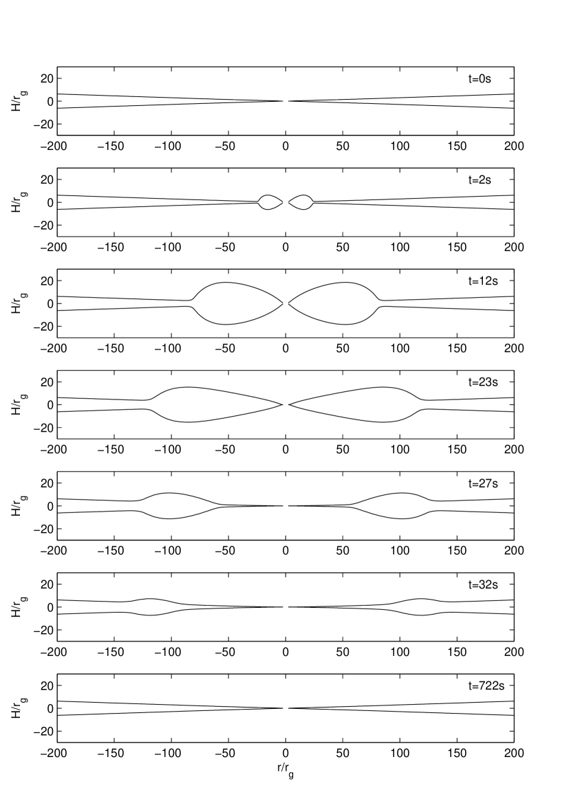
Figure 1: Evolution of the half-thickness of the disk during one full cycle.

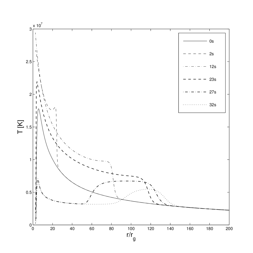
Figure 2: Evolution of the temperature of the matter in the disk during one full cycle.

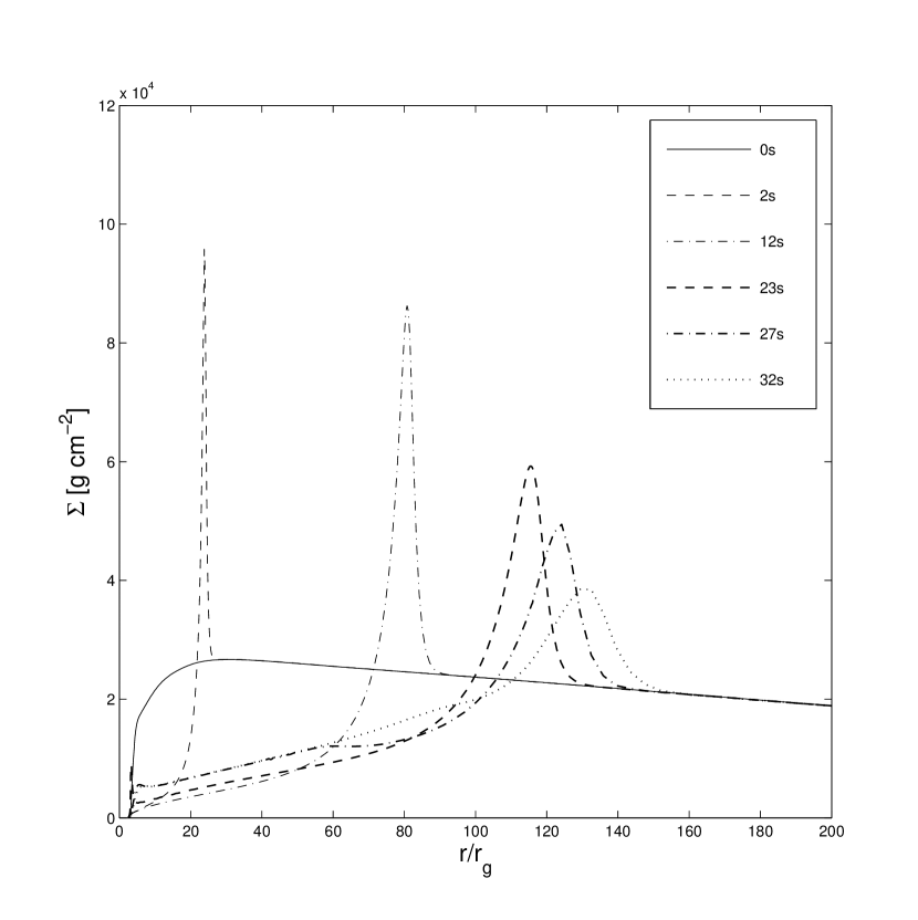
Figure 3: Evolution of the surface density of the disk.

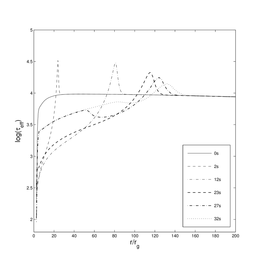
Figure 4: Evolution of the effective optical depth of the disk.

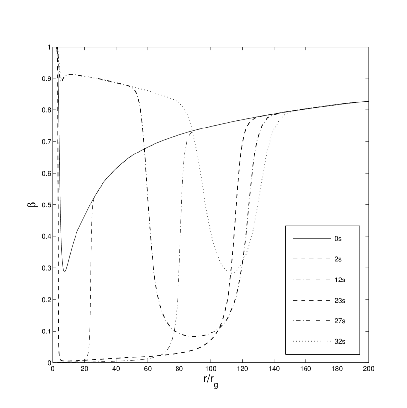
Figure 5: Evolution of the ratio of gas pressure to total pressure in the disk.

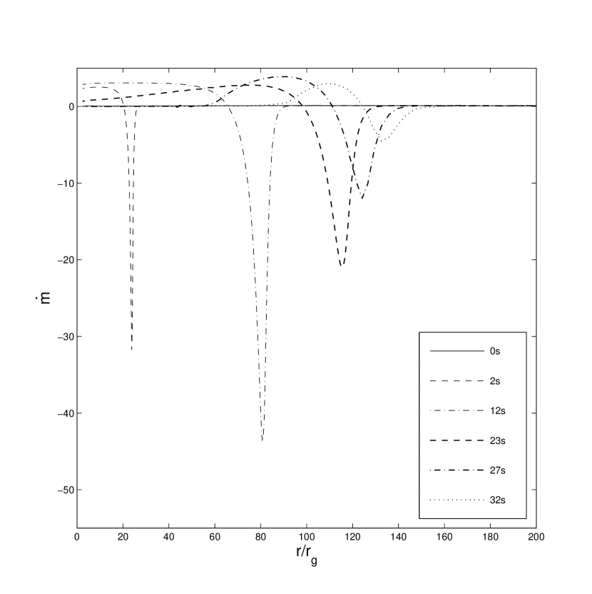
Figure 6: Evolution of the local accretion rate in the disk.

We have performed computations for a model accretion disk with black hole mass $M_{BH}=10M_{\odot}$, initial accretion rate $\dot{m}\equiv\dot{M}/\dot{M}_{cr}=0.06$ ($\dot{M}=-2\pi r\Sigma v_{r}$ is the accretion rate and $\dot{M}_{cr}$ is the critical accretion rate corresponding to the Eddington luminosity), and viscosity parameter $\alpha=0.1$ (the equivalent $\alpha$ in the diffusive viscosity prescription is $0.1\times(2/3\sqrt{6})\simeq 0.0272$). It is known that the inner region of a stationary accretion disk with such physical parameters is radiation pressure-supported ($\beta<0.4$) and is thermally unstable, and the disk is expected to exhibit the limit-cycle behavior (Kato et al., 1998, Chaps. 4 and 5). We have continued computations for several complete limit-cycles, and a representative cycle is illustrated in Figures 1 - 6, which are for the time evolution of the radial distribution of the half-thickness of the disk $H$, temperature $T$, surface density $\Sigma$, effective optical depth $\tau_{eff}=(2/3)(3\tau_{R}/2+\sqrt{3}+1/\tau_{P})$, ratio of gas pressure to total pressure $\beta$, and accretion rate $\dot{m}$, respectively. Note that negative values of $\dot{m}$ signify an outflow in the radial direction, not in the vertical direction as the word ’outflow’ in the literature usually means.

The first panel of Figure 1 and the solid lines in Figures 2 - 6 show the disk just before the start of the cycle ($t=0s$). The disk is essentially in the SSD state, i.e., it is geometrically thin ($H/r\ll 1$) and optically thick ($\tau_{eff}\gg 1$) everywhere, its temperature has a peak at $r\simeq 6r_{g}$, its accretion rate is nearly constant in space, and its inner region (from $\sim 5r_{g}$ to $\sim 14r_{g}$) has $\beta<0.4$ and is thermally unstable. Note that this configuration is not a stationary state and is with the diffusive viscosity prescription, so it is very different from the initial condition at the beginning of the computation, which is a stationary solution with the $\alpha p$ viscosity prescription.

As the instability sets in ($t=2s$, the second panel of Fig. 1 and the thin dashed lines in Figs. 2 - 6), in the unstable region ($r<24r_{g}$) the temperature rises rapidly, the disk expands in the vertical direction, a very sharp spike appears in the surface density profile and accordingly in the optical depth and accretion rate profiles (exactly the stiff problem). The spikes move outwards with time, forming an expansion wave, heating the inner material and pushing it into the black hole, and perturbing the outer material to departure from the SSD state. The expansion region is in fact essentially in the state of slim disk, as it is geometrically thick ($H/r\lesssim 1$), optically thick, very hot, and radiation pressure-supported ($\beta<0.4$); and the front of the expansion wave forms the transition surface between the SSD state and the slim disk state. At $t=12s$ (the third panel of Fig. 1 and the thin dot-dashed lines in Figs. 2 - 6), in the expansion region $H$ and $\dot{m}$ (negative, radial outflow) reach their maximum values, and the local $\dot{m}$ (positive, inflow) exceeds $3$ which is far above the initial value $\dot{m}=0.06$ and is even well above the critical value $\dot{m}=1$.

Once the wavefront has moved beyond the unstable region ($r\lesssim 120r_{g}$), the expansion starts to weaken, the temperature drops in the innermost part of the disk and the material there deflates ($t=23s$, the fourth panel of Fig. 1 and the thick dashed lines in Figs. 2 - 6). Subsequently, deflation spreads out through the disk, and the disk consists of three different parts: the inner part is geometrically thin, with the temperature and surface density being lower than their values at $t=0s$; the middle part is what remains of the slim disk state; and the outer part is still basically in the SSD state ($t=27s$, the fifth panel of Fig. 1 and the thick dot-dashed lines in Figs. 2 - 6).

The ’outburst’ part of the cycle ends when it has proceeded on the thermal time-scale ($t=32s$, the sixth panel of Fig. 1 and the dotted lines of Figs. 2 - 6). What follows is a much slower process (on the viscous time-scale) of refilling and reheating of the inner part of the disk. Finally ($t=722s$, the seventh panel of Fig. 1 and again the solid lines of Figs. 2 - 6), the disk returns to essentially the same state as that at the beginning of the cycle. Then the thermal instability occurs again and a new cycle starts.

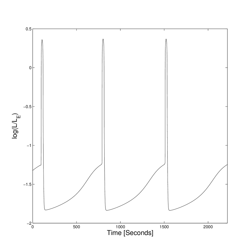
Figure 7: Variation of the bolometric luminosity of the disk during three full cycles.

The bolometric luminosity of the disk, obtained by integrating the radiated flux per unit area $F^{-}$ over the disk at successive times, is drawn in Figure 7 for three complete cycles. The luminosity exhibits a burst with a duration of about $20$ seconds and a quiescent phase lasting for the remaining about $700$ seconds of the cycle. The amplitude of the variation is around two orders of magnitude, during the outburst a super-Eddington luminosity is realized.

All these results obtained with our numerical method are similar to that of SM01, not only in the sense that the limit-cycle behavior of thermally unstable accretion disks is confirmed, but also in the sense that the numerical solutions are of very good quality. In our computations we have been able to suppress all numerical instabilities and to remove all spurious oscillations, so that in our figures all curves are perfectly continuous and smooth and all spikes are well-resolved.

What is new, however, is that we have also computed the Bernoulli function (i.e., the specific total energy) of the accreted matter that is expressed as (cf. Eq. [11.33] of Kato et al. 1998)

$$B=\left[3(1-\beta)+\frac{\beta}{\gamma-1}\right]\frac{p}{\rho}+\frac{1}{2}\left(v_{r}^{2}+V_{z}^{2}+\Omega^{2}r^{2}\right)-\frac{GM_{BH}}{\sqrt{r^{2}+H^{2}}-r_{g}}$$ (35)

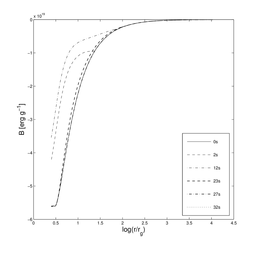
Figure 8: Bernoulli function of the matter of the disk. Note that the horizonal scale is very different from that in Figs. 1 - 6.

where $\gamma$ is the specific heat ratio and is taken to be $5/3$. Figure 8 shows the quantity $B$ obtained in the whole computational domain ranging from $r\simeq 2.5r_{g}$ to $r\simeq 10^{4}r_{g}$. It is clear that $B$ has negative values for the whole spatial range (approaching to zero for very large $r$) and during the whole time of the cycle (in the figure the thick dot-dashed line for $t=27s$ and the dotted line for $t=32s$ are coincided with the solid line for $t=0s$). Note that in equation (35) the vertical kinetic energy $0.5V_{z}^{2}$ is included, and the gravitational energy is that for the surface of the disk. If the vertical kinetic energy is omitted and the gravitational energy is taken to be its equatorial plane value as in 1-dimensional models, then $B$ will have even larger negative values. This result is in strong support of the analytical demonstration of Abramowicz et al. (2000) that accretion flows with not very strong viscosity ($\alpha\lesssim 0.1$) have a negative Bernoulli function; and implies that outflows are unlikely to originate from thermally unstable accretion disks we consider here, because a positive $B$ is a necessary, though not a sufficient, condition for the outflow production.

4 Summary and Discussion

We have introduced a numerical method for studies of thermally unstable accretion disks around black holes, which is essentially a combination of the standard one-domain pseudo-spectral method (Chan et al., 2005) and the adaptive domain decomposition method (Bayliss et al., 1995). As a test of our method, for the case of moderate viscosity we have reproduced the best numerical results obtained previously by SM01. Despite these similarities, we have made the following improvements over previous works in the numerical algorithm and concrete techniques, which have been proven to be effective in the practice of our computations.

1. In applying the domain decomposition method to resolve the stiff problem, we develop a simple and useful connection technique to ensure a numerically stable continuity for the derivative of a physical quantity across the interface of two conjoint subdomains, i.e., equations (13) and (14), instead of the connection technique in Bayliss et al. (1995) that is seemingly complicated and was not explicitly explained.

2. We construct a mapping function (eq. [15]) by adding the simple linear mapping function (eq. [16]) into the adaptive mapping function (eq. [17]) proposed by Bayliss et al. (1995), so that the mapping between the Chebyshev-Gauss-Lobatto collocation points $\bar{r}_{k}$ and the physical collocation points $r_{k}^{(i)}$, not only the mapping between two sets of collocation points $\bar{r}_{k}$ and $\tilde{r}_{k}$, is completed; and the adjustability of equation (17) is kept to enable us to follow adaptively the region that is with the stiff problem and is shifting in space during time-evolution.

3. For the time-integration, we use two complementary schemes, namely the third order TVD Runge-Kutta scheme and the third order backward-differentiation explicit scheme. The former scheme is popular in one-domain spectral methods and is essentially what was used by Chan et al. (2005), and the latter one can achieve the same accuracy and has advantage of lower CPU-time consumption.

4. For the treatment of boundary conditions, we notice that the spatial filter technique developed by Chan et al. (2005) for spectral methods is useful but is itself alone insufficient, and the treatment traditionally used in finite difference methods is still needed to complement. We also find that once reasonable conditions are set at the outer boundary, our solutions behave themselves physically consistent close to the black hole horizon, and no inner boundary conditions are necessary as supplied by SM01.

5. We resolve the problem of spurious oscillations due to the absence of viscous stress tensor components in the basic equations in a way different from that of SM01. SM01 introduced an artificial viscous term in the radial and vertical momentum equations. We instead improve the basic equations by including two viscous force terms $F_{rr}$ and $F_{\phi\phi}$ in the radial momentum equation and a corresponding viscous heating term in the energy equation, all these terms were already mentioned by the same authors of SM01 in an earlier paper (Szuszkiewicz & Miller, 1997). As for the vertical momentum equation, because of its crudeness in our $1.5$-dimensional studies, we still adopt an artificial term whose explicit form is kindly provided by Szuszkiewicz & Miller and is unpublished. We obtain solutions at the same quality level as in SM01, but we think that our treatment is probably more physical in some sense. In particular, any modification in the momentum equation ought to require a corresponding modification in the energy equation, otherwise the energy conservation would not be correctly described.

Of these five improvements, we expect that the first two and the last one will be particularly helpful for our subsequent studies of the strong viscosity case ($\alpha\sim 1$). In this case the viscous heating becomes extremely huge, the ’outburst’ of the disk due to the thermal instability is predicted to be more violent, and the Gibbs phenomenon related to the stiff problem can be even more serious than in the case of moderate viscosity studied in this paper. Our improved domain decomposition method is prepared to front these difficulties. As for another nettlesome problem that the absence of some viscous stress tensor components in $1$- or $1.5$-dimensional equations can also cause serious spurious oscillations, we think that, although in the moderate viscosity case they are equivalently effective as what were made by SM01, our modifications for both the radial momentum and energy equations will show their advantages in the strong viscosity case. In fact, the importance of the viscous forces $F_{rr}$ and $F_{\phi\phi}$ has long since been pointed out (e.g., Papaloizou & Stanley, 1986). We think that the inclusion of a heating term in the energy equation in accordance with these two forces will be not only consistent in physics, but also hopefully important in obtaining numerically stable solutions. With all these preparations made in this paper, we wish to achieve the goal to answer the question of the fate of thermally unstable black hole accretion disks with very large values of $\alpha$: do these disks finally form stable and persistent SSD+ADAF configurations as suggested by Takeuchi & Mineshige (1998), or they also undergo limit-cycles, or something else? In view of the two facts that limit-cyclic luminosity variations, even though with seemingly very reliable theoretical warranties, are not usually observed for black hole systems (GRS 1915+105 remains the only one known); and that outflows are already observed in many high energy astrophysical systems that are believed to be powered by black hole accretion, but are unlikely to originate from thermally unstable accretion disks we study here because of the negative Benoulli function of the matter in these disks, it will be definitely interesting if some behaviors other than the limit-cycle for non-stationary black hole accretion disks and/or the outflow formation from these disks can be demonstrated theoretically.

Appendix A Spectral Filtering and Boundary Conditions

When applied to solve non-linear partial differential equations, a principle drawback of spectral methods is the aliasing error that can cause spurious oscillations at high frequencies. The spectral filtering is a special technique developed to filter out the high-frequency modes in each time-step to reduce the aliasing error. As in Chan et al. (2005, see also ), we use a exponential filter in spectral space as

$$\sigma_{\delta}\left(\frac{n}{N}\right)\equiv\exp\left(-|\ln\epsilon|\left|\frac{n}{N}\right|^{\delta}\right),$$ (A1)

where $\epsilon$ is the machine accuracy and $\delta$ is a parameter that can be determined from the numerical practice. Then instead of $u(r_{k})$, the filtered collocation values of the physical quantity $u(r)$ at a collocation point $r_{k}$ are given by

$$\bar{u}(r_{k})=\sum\limits_{n=0}^{N}\sigma_{\delta}\left(\frac{n}{N}\right)\hat{u}_{n}\cos\left(\frac{nk\pi}{N}\right).$$ (A2)

As for the boundary conditions, the Dirichlet condition, $u|_{boundary}=u_{0}$, or/and the Neumann condition, $(\partial u/\partial r)|_{boundary}=u_{0}^{{}^{\prime}}$, are generally required. In order to avoid the appearance of discontinuous step-functions at the boundaries that would cause the Gibbs Phenomenon, Chan et al. (2005) introduced another filtering technique, namely the spatial filter. In our numerical algorithm, we either follow Chan et al. (2005) to impose the boundary conditions by using the spatial filter, or directly change the value of a certain physical quantity to be its given value at the boundary point, depending on whether the boundary derivative of the quantity is or is not very small. The spatial filter is a monotonically decreasing filter

$$h(r)=\exp\left[-|\ln\epsilon|\left(\frac{r-r_{min}}{r_{max}-r_{min}}\right)^{\delta}\right]$$ (A3)

for the outer boundary, and a monotonically increasing filter

$$h(r)=\exp\left[-|\ln\epsilon|\left(\frac{r_{max}-r}{r_{max}-r_{min}}\right)^{\delta}\right]$$ (A4)

for the inner boundary. With this filter, the Dirichlet boundary condition can be imposed in each time-step as

$$u_{k}^{n}\rightarrow(u_{k}^{n}-u_{0})h(r_{k})+u_{0},$$ (A5)

and the Neumann boundary condition can be imposed as

$$\left(\frac{\partial u}{\partial r}\right)_{k}^{n}\rightarrow\left[\left(\frac{\partial u}{\partial r}\right)_{k}^{n}-u_{0}^{{}^{\prime}}\right]h(r_{k})+u_{0}^{{}^{\prime}},$$ (A6)

where the superscript $n$ and subscript $k$ denote the relevant values at the $n$-th time-level and the collocation point $r_{k}$, respectively.

References

- Abramowicz et al. (2000) Abramowicz, M. A., Lasota, J.-P., & Igumenshchev, I. V. 2000, MNRAS, 314, 775
- Abramowicz et al. (1995) Abramowicz, M. A., Chen, X., Kato, S., Lasota, J.-P., & Regev, O. 1995, ApJ, 438, L37
- Abramowicz et al. (1988) Abramowicz, M. A., Czerny, B., Lasota, J.-P., & Szuszkiewicz, E. 1988, ApJ, 332, 646
- Bayliss et al. (1995) Bayliss, A., Garbey, M., & Matkowsky, B. 1995, J. Comput. Phys., 119, 132
- Becker & Subramanian (2005) Becker, P. A., & Subramanian, P. 2005, ApJ, 622, 520
- Boyd (2000) Boyd, J.P. 2000, Chebyshev and Fourier Spectral Methods, 2nd Edition (New York: Dover)
- Chan et al. (2005) Chan, C.-K., Psaltis, D., & Özel, F. 2005, ApJ, 628, 353
- Chan et al. (2006) Chan, C.-K., Psaltis, D., & Özel, F. 2006, ApJ, 645, 506
- Chen et al. (1995) Chen, X., Abramowicz, M. A., Lasota, J.-P., Narayan, R., & Yi, I. 1995, ApJ, 443, L61
- Canuto et al. (1988) Canuto, C., Hussaini, M.Y., Quarteroni, A., & Zang, T.A. 1988, Spectral Methods in Fluid Dynamics (New York: Springer)
- Gottlieb & Orszag (1983) Gottlieb, D., & Orszag, S.A. 1983, Numerical Analysis of Spectral Methods: Theory and Applications (Philadelphia: SIAM)
- Gottlieb & Shu (1997) Gottlieb, D., & Shu, C.-W. 1997, SIAM Rev., 39(4), 644
- Hawley et al. (2001) Hawley, J. F., Balbus, S.A., & Stone, J.M. 2001, ApJ, 554, L49
- Honma et al. (1991) Honma, F., Matsumoto, R., & Kato, S. 1991, PASJ, 43, 147
- Janiuk et al. (2002) Janiuk, A., Czerny, B., & Siemiginowska, A. 2002, ApJ, 576, 908
- Kato et al. (1998) Kato, S., Fukue, J., & Mineshige, S. 1998, Black-Hole Accretion Disks (Kyoto: Kyoto Univ. Press)
- Kawata et al. (2006) Kawata, A., Watarai, K., & Fukue, J. 2006, PASJ, 58, 447
- Mayer & Pringle (2006) Mayer, M., & Pringle, J. E. 2006, MNRAS, 368, 396
- Narayan et al. (1998) Narayan, R., Mahadevan, R., & Quataert, E. 1998, in The Theory of Black Hole Accretion Disks, ed. M. A. Abramowicz, G. Björnsson, & J. E. Pringle (Cambridge: Cambridge Univ. Press), 148
- Narayan & Yi (1994) Narayan, R., & Yi, I. 1994, ApJ, 428, L13
- Nayakshin et al. (2000) Nayakshin, S., Rappaport, S., & Melia, F. 2000, ApJ, 535, 798
- Ohsuga (2006) Ohsuga, K. 2006, ApJ, 640, 923
- Papaloizou & Stanley (1986) Papaloizou J. C. B., & Stanley G. Q. C. 1986, MNRAS, 220, 593
- Peyret (2002) Peyret, R. 2002, Spectral Methods for Incompressible Viscous Flow (New York: Springer)
- Press et al. (1992) Press, W.H., Teukolsky, S.A., Vetterling, W.T., & Flannery, B.P. 1992, Numerical recipes in FORTRAN: the art of scientific computing, 2nd Edition (New York: Cambridge University Press)
- Shakura & Sunyaev (1973) Shakura, N.I., & Sunyaev, R.A. 1973, A&A, 24, 337
- Shu & Osher (1988) Shu, C.W.,& Osher, S. 1988, J. Comput. Phys., 77, 439
- Szuszkiewicz & Miller (1997) Szuszkiewicz, E., & Miller, J.C. 1997, MNRAS, 287, 165
- Szuszkiewicz & Miller (1998) Szuszkiewicz, E., & Miller, J.C. 1998, MNRAS, 298, 888
- Szuszkiewicz & Miller (2001) Szuszkiewicz, E., & Miller, J.C. 2001, MNRAS, 328, 36 (SM01)
- Takeuchi & Mineshige (1998) Takeuchi, M., & Mineshige, S. 1998, ApJ, 505, L19
- Teresi et al. (2004a) Teresi, V., Molteni, D., & Toscano, E. 2004a, MNRAS, 348, 361
- Teresi et al. (2004b) Teresi, V., Molteni, D., & Toscano, E. 2004b, MNRAS, 351, 297
- Watarai & Mineshige (2003) Watarai K., & Mineshige S. 2003, ApJ, 596, 421