Unequal dimensional small balls and quantization on Grassmann Manifolds${}^{{}^{*}}$

Abstract

The Grassmann manifold $\mathcal{G}_{n,p}\left(\mathbb{L}\right)$ is the set of all $p$-dimensional planes (through the origin) in the $n$-dimensional Euclidean space $\mathbb{L}^{n}$, where $\mathbb{L}$ is either $\mathbb{R}$ or $\mathbb{C}$. This paper considers an unequal dimensional quantization in which a source in $\mathcal{G}_{n,p}\left(\mathbb{L}\right)$ is quantized through a code in $\mathcal{G}_{n,q}\left(\mathbb{L}\right)$, where $p$ and $q$ are not necessarily the same. It is different from most works in literature where $p\equiv q$. The analysis for unequal dimensional quantization is based on the volume of a metric ball in $\mathcal{G}_{n,p}\left(\mathbb{L}\right)$ whose center is in $\mathcal{G}_{n,q}\left(\mathbb{L}\right)$. Our chief result is a closed-form formula for the volume of a metric ball when the radius is sufficiently small. This volume formula holds for Grassmann manifolds with arbitrary $n$, $p$, $q$ and $\mathbb{L}$, while previous results pertained only to some special cases. Based on this volume formula, several bounds are derived for the rate distortion tradeoff assuming the quantization rate is sufficiently high. The lower and upper bounds on the distortion rate function are asymptotically identical, and so precisely quantify the asymptotic rate distortion tradeoff. We also show that random codes are asymptotically optimal in the sense that they achieve the minimum achievable distortion with probability one as $n$ and the code rate approach infinity linearly.

Finally, we discuss some applications of the derived results to communication theory. A geometric interpretation in the Grassmann manifold is developed for capacity calculation of additive white Gaussian noise channel. Further, the derived distortion rate function is beneficial to characterizing the effect of beamforming matrix selection in multi-antenna communications.

I Introduction

The Grassmann manifold $\mathcal{G}_{n,p}\left(\mathbb{L}\right)$ is the set of all $p$-dimensional planes (through the origin) in the $n$-dimensional Euclidean space $\mathbb{L}^{n}$, where $\mathbb{L}$ is either $\mathbb{R}$ or $\mathbb{C}$. It forms a compact Riemann manifold of real dimension $\beta p\left(n-p\right)$, where $\beta=1$ when $\mathbb{L}=\mathbb{R}$ and $\beta=2$ when $\mathbb{L}=\mathbb{C}$. The Grassmann manifold is a useful analysis tool for multi-antenna communications (also known as multiple-input multiple-output (MIMO) communication systems). The capacity of non-coherent MIMO systems at high signal-to-noise ratio (SNR) region was derived by analysis in the Grassmann manifold [2]. The well known spherical codes for MIMO systems can be viewed as codes in the Grassmann manifold [3]. Further, for coherent MIMO systems with finite rate feedback, the quantization of eigen-channel vectors is related to the quantization on the Grassmann manifold [4, 5, 6, 7, 8].

This paper studies unequal dimensional quantization on the Grassmann manifold. Roughly speaking, a quantization is a representation of a source: it maps an element in $\mathcal{G}_{n,p}\left(\mathbb{L}\right)$ (the source) into a subset $\mathcal{C}\subset\mathcal{G}_{n,q}\left(\mathbb{L}\right)$, which is often discrete and referred to as a code. While it is traditionally assumed that $p\equiv q$ [9, 10, 11, 1], we are interested in a more general case where $p$ may not necessarily equal to $q$; thus the term unequal dimensional quantization. The performance limit of quantization is given by the so called rate distortion tradeoff. Let the source be randomly distributed and define a distortion metric between elements in $\mathcal{G}_{n,p}\left(\mathbb{L}\right)$ and $\mathcal{G}_{n,q}\left(\mathbb{L}\right)$. The rate distortion tradeoff is described by the minimum average distortion achievable for a given code size, or equivalently the minimum code size required to achieve a particular average distortion. This paper will quantify the rate distortion tradeoff for unequal dimensional quantization.

This paper appears to be the first to explore unequal dimensional quantization systematically. According to the authors’ knowledge, works in literature assume that $p=q$: The Rankin bound in $\mathcal{G}_{n,p}\left(\mathbb{R}\right)$ is obtained in [9] when the code size is large. When $p$ is fixed and $n$ is asymptotically large, approximations to the Gilbert-Varshamov and Hamming bounds on $\mathcal{G}_{n,p}\left(\mathbb{L}\right)$ are drived by Laplace method in [10] and by volume estimates in [11, 12]. The distortion rate tradeoff for the $p=1$ case is quantified in [4, 5] by direct volume calculation and in [7] using high resolution quantization theory. Our paper [1] characterizes the tradeoff for the general $p$ case when quantization rate is sufficiently high. While the $p=q$ case has been extensively studied, unequal dimensional quantization does arise in some multi-antenna communication systems, see [8] for an example. It is thus worthwhile to go beyond the $p=q$ case.

The main contribution of this paper is to derive a closed-form formula for the volume of a small ball in the Grassmann manifold and then accurately quantify the rate distortion tradeoff accordingly. Specifically:

1. An explicit volume formula for a metric ball is derived for arbitrary $n$, $p$, $q$ and $\mathbb{L}$ when the radius $\delta$ is sufficiently small. Useful lower and upper bounds on the volume are also presented.

2. Tight lower and upper bounds are derived for the rate distortion tradeoff. Further, fix $p$ and $q$ but let $n$ and the code rate (logarithm of the code size) approach infinity linearly. The lower and upper bounds are in fact asymptotically identical, and so precisely quantify the asymptotic rate distortion tradeoff. We also show that random codes are asymptotically optimal in the sense that they achieve the minimum achievable distortion with probability one in this asymptotic region.

Finally, some applications of the derived results to communication theory are presented. We show that data transmission in additive white Gaussian noise (AWGN) channel is essentially communication on the Grassmann manifold. A geometric interpretation for AWGN channel is developed in the Grassmann manifold accordingly. Moreover, the beamforming matrix selection in a MIMO system is closely related to quantization on the Grassmann manifold. The results for the distortion rate tradeoff are therefore helpful to characterize the effect of beamforming matrix selection.

II Preliminaries

For the sake of applications [4, 5, 6], the projection Frobenius metric (chordal distance) and the invariant measure on the Grassmann manifold are employed throughout this paper. Without loss of generality, we assume that $p\leq q$. For any two planes $P\in\mathcal{G}_{n,p}\left(\mathbb{L}\right)$ and $Q\in\mathcal{G}_{n,q}\left(\mathbb{L}\right)$, we define the principle angles and the chordal distance between $P$ and $Q$ as follows. Let $\mathbf{p}_{1}\in P$ and $\mathbf{q}_{1}\in Q$ be the unit vectors such that $\left|\mathbf{p}_{1}^{\dagger}\mathbf{q}_{1}\right|$ is maximal. Inductively, let $\mathbf{p}_{i}\in P$ and $\mathbf{q}_{i}\in Q$ be the unit vectors such that $\mathbf{p}_{i}^{\dagger}\mathbf{p}_{j}=0$ and $\mathbf{q}_{i}^{\dagger}\mathbf{q}_{j}=0$ for all $1\leq j<i$ and $\left|\mathbf{p}_{i}^{\dagger}\mathbf{q}_{i}\right|$ is maximal. The principle angles are then defined as $\theta_{i}=\arccos\left|\mathbf{p}_{i}^{\dagger}\mathbf{q}_{i}\right|$ for $i=1,\cdots,p$ [9], and the chordal distance between $P$ and $Q$ is then given by

$$d_{c}\left(P,Q\right)\triangleq\sqrt{\sum_{i=1}^{p}\sin^{2}\theta_{i}}.$$ (1)

The invariant measure $\mu$ on $\mathcal{G}_{n,p}\left(\mathbb{L}\right)$ is the Haar measure on $\mathcal{G}_{n,p}\left(\mathbb{L}\right)$. Let $O\left(n\right)$ and $U\left(n\right)$ be the groups of $n\times n$ orthogonal and unitary matrices respectively. Let $\mathbf{A},\mathbf{B}\in O\left(n\right)$ when $\mathbb{L}=\mathbb{R}$, or $\mathbf{A},\mathbf{B}\in U\left(n\right)$ when $\mathbb{L}=\mathbb{C}$. For any measurable set $\mathcal{M}\subset\mathcal{G}_{n,p}\left(\mathbb{L}\right)$ and arbitrary $\mathbf{A}$ and $\mathbf{B}$, $\mu$ satisfies

$$\mu\left(\mathbf{A}\mathcal{M}\right)=\mu\left(\mathcal{M}\right)=\mu\left(\mathcal{M}\mathbf{B}\right).$$

The invariant measure defines the uniform/isotropic distribution on $\mathcal{G}_{n,p}\left(\mathbb{L}\right)$ [13].

This paper addresses an unequal dimensional quantization problem. Let $\mathcal{C}$ be a finite size discrete subset of $\mathcal{G}_{n,q}\left(\mathbb{L}\right)$ (also known as a code). An unequal dimensional quantization is a mapping from the $\mathcal{G}_{n,p}\left(\mathbb{L}\right)$ to the set $\mathcal{C}$, $\mathfrak{q}:\mathcal{G}_{n,p}\left(\mathbb{L}\right)\rightarrow\mathcal{C}$, where $p$ and $q$ are not necessarily the same integer. Without loss of generality, we assume $p\leq q$. We are interested in quantifying the rate distortion tradeoff. Assume that a source $P\in\mathcal{G}_{n,p}\left(\mathbb{L}\right)$ is isotropically distributed. Define the distortion measure as the square of the chordal distance $d_{c}^{2}\left(\cdot,\cdot\right)$. Then the distortion associated with a quantization $\mathfrak{q}$ is defined as $D\triangleq\mathrm{E}_{P}\left[d_{c}^{2}\left(P,\mathfrak{q}\left(P\right)\right)\right].$ For a given code $\mathcal{C}\subset\mathcal{G}_{n,q}\left(\mathbb{L}\right)$, the optimal quantization to minimize the distortion is given by $\mathfrak{q}\left(P\right)=\arg\;\underset{Q\in\mathcal{C}}{\min}\;d_{c}\left(P,Q\right).$ The corresponding distortion is

$$D\left(\mathcal{C}\right)=\mathrm{E}_{P}\left[\underset{Q\in\mathcal{C}}{\min}\;d_{c}^{2}\left(P,Q\right)\right].$$

The rate distortion tradeoff can be described by the distortion rate function: the infimum achievable distortion given a code size $K$

$$D^{*}\left(K\right)=\underset{\mathcal{C}:\left|\mathcal{C}\right|=K}{\inf}\;D\left(\mathcal{C}\right),$$ (2)

or the rate distortion function: the minimum required code size to achieve a given distortion $D$

$$K^{*}\left(D\right)=\underset{D\left(\mathcal{C}\right)\leq D}{\inf}\;\left|\mathcal{C}\right|.$$ (3)

III Metric Balls in the Grassmann Manifold

This section derives an explicit volume formula for a metric ball $B\left(\delta\right)$ in the Grassmann manifold. It is the essential tool to quantify the rate distortion tradeoff.

The volume of a ball can be expressed as a multivariate integral. Assume the invariant measure $\mu$ and the chordal distance $d_{c}$. For any given $P\in\mathcal{G}_{n,p}\left(\mathbb{L}\right)$ and $Q\in\mathcal{G}_{n,q}\left(\mathbb{L}\right)$, define

$$B_{P}\left(\delta\right)=\left\{\hat{Q}\in\mathcal{G}_{n,q}\left(\mathbb{L}\right):\;d_{c}\left(P,\hat{Q}\right)\leq\delta\right\}$$

and

$$B_{Q}\left(\delta\right)=\left\{\hat{P}\in\mathcal{G}_{n,p}\left(\mathbb{L}\right):\;d_{c}\left(\hat{P},Q\right)\leq\delta\right\}.$$

It has been shown that $\mu\left(B_{P}\left(\delta\right)\right)=\mu\left(B_{Q}\left(\delta\right)\right)$ and the value is independent of the choice of the center [13]. For convenience, we denote $B_{P}\left(\delta\right)$ and $B_{Q}\left(\delta\right)$ by $B\left(\delta\right)$ without distinguishing them. Then, the volume of a metric ball $B\left(\delta\right)$ is given by

$$\mu\left(B\left(\delta\right)\right)=\underset{\sum_{i=1}^{p}\sin^{2}\theta_{i}\leq\delta^{2}}{\int\cdots\int}\;d\mu_{\bm{\theta}},$$ (4)

where $1\leq\theta_{1}\leq\frac{\pi}{2},\cdots,1\leq\theta_{p}\leq\frac{\pi}{2}$ are the principle angles and the differential form $d\mu_{\bm{\theta}}$ is the joint density of the $\theta_{i}$’s [13, 14].

Theorem 1 computes the multivariate integral (4) into a simple exponential form.

Theorem 1

When $\delta\leq 1$, the volume of a metric ball $B\left(\delta\right)$ is given by

$$\mu\left(B\left(\delta\right)\right)=c_{n,p,q,\beta}\delta^{\beta p\left(n-q\right)}\left(1+c_{n,p,q,\beta}^{\left(1\right)}\delta^{2}+o\left(\delta^{2}\right)\right),$$ (5)

where

$$\beta=\left\{\begin{array}[]{ll}1&\mathrm{if}\;\mathbb{L}=\mathbb{R}\\ 2&\mathrm{if}\;\mathbb{L}=\mathbb{C}\end{array}\right.,$$

$$c_{n,p,q,\beta}=\left\{\begin{array}[]{l}\frac{1}{\Gamma\left(\frac{\beta}{2}p\left(n-q\right)+1\right)}\prod_{i=1}^{p}\frac{\Gamma\left(\frac{\beta}{2}\left(n-i+1\right)\right)}{\Gamma\left(\frac{\beta}{2}\left(q-i+1\right)\right)}\\ \quad\quad\quad\quad\quad\quad\quad\quad\quad\quad\;\mathrm{if}\;p+q\leq n\\ \frac{1}{\Gamma\left(\frac{\beta}{2}p\left(n-q\right)+1\right)}\prod_{i=1}^{n-q}\frac{\Gamma\left(\frac{\beta}{2}\left(n-i+1\right)\right)}{\Gamma\left(\frac{\beta}{2}\left(n-p-i+1\right)\right)}\\ \quad\quad\quad\quad\quad\quad\quad\quad\quad\quad\;\mathrm{if}\;p+q\geq n\end{array}\right.,$$ (6)

and

$$c_{n,p,q,\beta}^{\left(1\right)}=-\left(\frac{\beta}{2}\left(q-p+1\right)-1\right)\frac{\frac{\beta}{2}p\left(n-q\right)}{\frac{\beta}{2}p\left(n-q\right)+1}.$$ (7)

The proof is given in the journal version of this paper [15].

There are two cases where the volume formula becomes exact.

Corollary 1

When $\delta\leq 1$, in either of the following two cases,

1. $\mathbb{L}=\mathbb{C}$ and $q=p$;

2. $\mathbb{L}=\mathbb{R}$ and $q=p+1$,

the volume of a metric ball $B\left(\delta\right)$ is exactly

$$\mu\left(B\left(\delta\right)\right)=c_{n,p,q,\beta}\delta^{\beta p\left(n-q\right)},$$

where $c_{n,p,q,\beta}$ is defined in (6).

We also have the general bounds:

Corollary 2

Assume $\delta\leq 1$. If $\mathbb{L}=\mathbb{R}$ and $p=q$ , the volume of $B\left(\delta\right)$ is bounded by

$$c_{n,p,p,1}\delta^{p\left(n-p\right)}\leq\mu\left(B\left(\delta\right)\right)\leq c_{n,p,p,1}\delta^{p\left(n-p\right)}\left(1-\delta^{2}\right)^{-\frac{p}{2}}.$$

For all other cases,

$$\left(1-\delta^{2}\right)^{\frac{\beta}{2}p\left(q-p+1\right)-p}c_{n,p,q,\beta}\delta^{\beta p\left(n-q\right)}$$

$$\quad\quad\leq\mu\left(B\left(\delta\right)\right)\leq c_{n,p,q,\beta}\delta^{\beta p\left(n-q\right)}.$$

Proof:

Corollary 1 and 2 follow the proof of Theorem 1 by tracking the higher order terms. ∎

Theorem 1 is of course consistent with the previous results in [1, 10, 4], which pertain to special choices of $n$, $p$, $q$ or $\mathbb{L}$. Importantly though, Theorem 1 is distinct in that it holds for arbitrary $n,$ $p$, $q$ and $\mathbb{L}$.

For engineering purposes, it is often satisfactory to approximate the volume of a metric ball $B\left(\delta\right)$ by $c_{n,p,q,\beta}\delta^{\beta p\left(n-q\right)}$ when $\delta\leq 1$. Fig. 1 compares the simulated volume (4) and the approximation $c_{n,p,q,\beta}\delta^{\beta p\left(n-q\right)}$. Since it is often difficult to directly evaluate the multivariate integral in (4), we simulate $\mu\left(B\left(\delta\right)\right)=\Pr\left\{\hat{P}\in\mathcal{G}_{n,p}\left(\mathbb{L}\right):\;d_{c}\left(\hat{P},Q\right)\leq\delta\right\}$ by fixing $Q$ and generating isotropically distributed $\hat{P}$. The simulation results show that our volume approximation $c_{n,p,q,\beta}\delta^{\beta p\left(n-q\right)}$ (solid lines) is close to the simulated volume (circles) when $\delta\leq 1$. We also compare our approximation with Barg-Nogin approximation developed in [10]. There, an volume approximation $\left(\delta/\sqrt{p}\right)^{\beta np}$ is derived by Laplace method and is only valid for the $p=q\ll n$. Simulations show that the simulated volume and Barg-Nogin approximation (dash lines) may not be of the same order while our approximation is much more accurate.

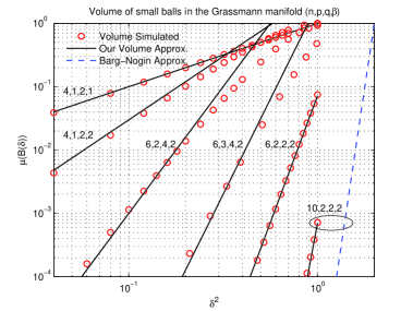
Figure 1: Volume of small balls in the Grassmann manifold. The integers besides curves are, from left to right, $n,\;p,\;q,\;\mathrm{and}\;\beta$ respectively.

IV Quantization Bounds

This section quantifies the rate distortion tradeoff for the unequal dimensional quantization problem. The results hold for arbitrary $n$, $p$, $q$ and $\mathbb{L}$.

Recall the distortion rate function defined in (2). A lower bound and an upper bound are derived.

Theorem 2

When $K$ is sufficiently large ($\left(c_{n,p,q,\beta}K\right)^{-\frac{2}{\beta p\left(n-q\right)}}\leq 1$ necessarily), the distortion rate function is bounded as in

$$\frac{\beta p\left(n-q\right)}{\beta p\left(n-q\right)+2}\left(c_{n,p,q,\beta}K\right)^{-\frac{2}{\beta p\left(n-q\right)}}\left(1+o\left(1\right)\right)\leq D^{*}\left(K\right)$$

$$\quad\quad\quad\leq\frac{2\Gamma\left(\frac{2}{\beta p\left(n-q\right)}\right)}{\beta p\left(n-q\right)}\left(c_{n,p,q,\beta}K\right)^{-\frac{2}{\beta p\left(n-q\right)}}\left(1+o\left(1\right)\right).$$ (8)

Remark 1

For engineering purposes, the main order terms in (8) are usually accurate enough to characterize the distortion rate function. The details of the $\left(1+o\left(1\right)\right)$ correction are spelled out in the journal version of this paper [15].

The proof is provided in the journal version of this paper [15]. We sketch it as follows.

The lower bound is proved by a sphere covering argument. The key is to construct an ideal quantizer, which may not exist, to minimize the distortion. Suppose that there exists $K$ metric balls of the same radius $\delta_{0}$ packing and covering the whole $\mathcal{G}_{n,p}\left(\mathbb{L}\right)$ at the same time. Then the quantizer which maps each of those balls into its center $Q\in\mathcal{G}_{n,q}\left(\mathbb{L}\right)$ gives the minimum distortion among all quantizers. Of course such an ideal covering may not exist. Therefore, the corresponding distortion may not be achievable. It is only a lower bound on the distortion rate function.

Next the upper bound is obtained by calculating the average distortion of random codes. The basic idea is that the distortion of any particular code is an upper bound of the distortion rate function and so is the average distortion of random codes. A random code $\mathcal{C}_{\mathrm{rand}}=\left\{Q_{1},\cdots,Q_{K}\right\}$ is generated by drawing the codewords $Q_{i}$’s independently from the isotropic distribution on $\mathcal{G}_{n,q}\left(\mathbb{L}\right)$. The average distortion of random codes is given by $\mathrm{E}_{\mathcal{C}_{\mathrm{rand}}}\left[D\left(\mathcal{C}_{\mathrm{rand}}\right)\right]$. By extreme order statistics, see for example [16], the calculation of $\mathrm{E}_{\mathcal{C}_{\mathrm{rand}}}\left[D\left(\mathcal{C}_{\mathrm{rand}}\right)\right]$ is directly related to the volume (4). Based on our volume formula (5), the asymptotic value of $\mathrm{E}_{\mathcal{C}_{\mathrm{rand}}}\left[D\left(\mathcal{C}_{\mathrm{rand}}\right)\right]$ is computed and thus the upper bound is obtained for large $K$.

As the dual part of the distortion rate tradeoff, lower and upper bounds are constructed for the rate distortion function.

Corollary 3

When the required distortion $D$ is sufficiently small ($D\leq 1$ necessarily), the rate distortion function satisfies the following bounds,

$$\frac{1}{c_{n,p,q,\beta}}\left(\frac{\beta p\left(n-q\right)}{2\Gamma\left(\frac{2}{\beta p\left(n-q\right)}\right)}D\right)^{-\frac{\beta p\left(n-q\right)}{2}}\left(1+o\left(1\right)\right)\leq K^{*}\left(D\right)$$

$$\quad\quad\leq\frac{1}{c_{n,p,q,\beta}}\left(\frac{\beta p\left(n-q\right)+2}{\beta p\left(n-q\right)}D\right)^{-\frac{\beta p\left(n-q\right)}{2}}\left(1+o\left(1\right)\right).$$ (9)

It is interesting to observe that the lower and upper bounds are asymptotically the same. As a result, the asymptotic rate distortion tradeoff is exactly quantified.

Theorem 3

Suppose that $p$ and $q$ are fixed. Let $n$ and the code rate $\log_{2}K$ approach infinity linearly with $\frac{\log_{2}K}{n}\rightarrow\bar{r}$. If the normalized code rate $\bar{r}$ is sufficiently large ($p2^{-\frac{2}{\beta p}\bar{r}}\leq 1$ necessarily), then

$$\underset{\left(n,K\right)\rightarrow+\infty}{\lim}D^{*}\left(K\right)=p2^{-\frac{2}{\beta p}\bar{r}}.$$

On the other hand, if the required distortion $D$ is sufficiently small ($D\leq 1$ necessarily), then the minimum code size required to achieve the distortion $D$ satisfies

$$\underset{n\rightarrow+\infty}{\lim}\frac{\log_{2}K^{*}\left(D\right)}{n}=\frac{\beta p}{2}\log_{2}\left(\frac{p}{D}\right).$$ (10)

Remark 2

That the $\left(1+o\left(1\right)\right)$ multiplicative errors in (8) and (9) disappear is the content of [15]. We omit the corresponding details due to the space limitation.

Fig. 2 compares the simulated distortion rate function (the plus markers) with its lower bound (the dashed lines) and upper bound (the solid lines) in (8). To simulate the distortion rate function, we use the max-min criterion to design codes and the employ the corresponding distortion as an estimate of the distortion rate function. Simulation results show that the bounds in (8) hold for large $K$. When $K$ is relatively small, the formula (8) can serve as good approximations to the distortion rate function as well. Furthermore, we compare our bounds with the approximation (the “x” markers) derived in [17], which is partly based on Barg-Nogin volume approximation. Simulations show that the approximation in [17] is neither an upper bound nor a lower bound. It works for the case that $n=10$ and $p=2$ but doesn’t work when $n\leq 8$ and $p=2$. As a comparison, our bounds (8) hold for arbitrary $n$ and $p$.

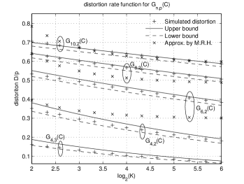
Figure 2: Bounds on the distortion rate function

While the asymptotic rate distortion tradeoff is precisely quantified, the next question could be how to achieve it. Same to many cases in information theory, random codes are asymptotically optimal with probability one.

Corollary 4

Consider unequal dimensional quantization from $\mathcal{G}_{n,p}\left(\mathbb{L}\right)$ to $\mathcal{G}_{n,q}\left(\mathbb{L}\right)$. Let $\mathcal{C}_{\mathrm{rand}}\subset\mathcal{G}_{n,q}\left(\mathbb{L}\right)$ be a code randomly generated from the isotropic distribution and with size $K$. Fix $p$ and $q$. Let $n,\log_{2}K\rightarrow\infty$ with $\frac{\log_{2}K}{n}\rightarrow\bar{r}\in\mathbb{R}^{+}$. If the normalized code rate $\bar{r}$ is sufficiently large ($p2^{-\frac{2}{\beta p}\bar{r}}\leq 1$ necessarily), then for $\forall\epsilon>0$,

$$\underset{\left(n,K\right)\rightarrow\infty}{\lim}\Pr\left(D\left(\mathcal{C}_{\mathrm{rand}}\right)>p2^{-\frac{2}{\beta p}\bar{r}}+\epsilon\right)=0$$

The proof is omitted due to the space limitation.

V Applications to Communication Theory

V-A Channel Capacity of AWGN Channel

Although the capacity of AWGN channel is well known, it is interesting to re-calculate it from an interpretation in the Grassmann manifold.

The signal transmission model for an AWGN channel is that $\mathbf{Y}=\mathbf{X}+\mathbf{W},$ where $\mathbf{Y},\;\mathbf{X},\;\mathbf{W}\in\mathbb{L}^{n}$ are the received signal, the transmitted signal and the additive Gaussian noise respectively, and $\mathbb{L}$ is either $\mathbb{R}$ or $\mathbb{C}$. Assume that $\mathbf{X}$ and $\mathbf{W}$ are Gaussian vectors with zero mean and covariance matrices $\mathrm{E}\left[\mathbf{XX}^{\dagger}\right]=\mathbf{I}$ and $\mathrm{E}\left[\mathbf{WW}^{\dagger}\right]=\sigma^{2}\mathbf{I}$ respectively. For any $\epsilon>0$, construct a random codebook $\mathcal{B}_{\mathbf{X}}=\left\{\mathbf{X}_{1},\cdots,\mathbf{X}_{K}\right\}$ with $\frac{\log_{2}K}{n}\rightarrow R_{\epsilon}$ and $\frac{1}{n}\left\|\mathbf{X}_{k}\right\|^{2}\in\left(1-2\epsilon,1-\epsilon\right)$ for all $k=1,\cdots,K$.

Now suppose that a codeword $\mathbf{X}_{1}$ is transmitted. We consider a receiver given by

$$\hat{\mathbf{X}}=\underset{\mathbf{X}\in\mathcal{B}_{\mathbf{X}}}{\arg\;\min}\;d_{c}^{2}\left(\mathcal{P}\left(\mathbf{X}\right),\mathcal{P}\left(\mathbf{Y}\right)\right),$$

where $\mathcal{P}\left(\mathbf{X}\right)\in\mathcal{G}_{n,1}\left(\mathbb{L}\right)$ and $\mathcal{P}\left(\mathbf{Y}\right)\in\mathcal{G}_{n,1}\left(\mathbb{L}\right)$ are planes generated by $\mathbf{X}$ and $\mathbf{Y}$ respectively. It can be verified that

$$\frac{\sigma^{2}}{1+\sigma^{2}-\epsilon}\leq\underset{n\rightarrow\infty}{\lim}d_{c}^{2}\left(\mathcal{P}\left(\mathbf{X}_{1}\right),\mathcal{P}\left(\mathbf{Y}\right)\right) \leq\frac{\sigma^{2}}{1+\sigma^{2}-2\epsilon}.$$

By similar argument to the proof of Theorem 2, if

$$R_{\epsilon}<\underset{n\rightarrow\infty}{\lim}\frac{\log_{2}K^{*}\left(\frac{\sigma^{2}}{1+\sigma^{2}-2\epsilon}\right)}{n}=\frac{\beta}{2}\log\left(1+\frac{1-2\epsilon}{\sigma^{2}}\right),$$

then $\Pr\left(\hat{\mathbf{X}}\neq\mathbf{X}_{1}\right)=\Pr\left(\exists j\neq 1,\;d_{c}^{2}\left(\mathcal{P}\left(\mathbf{X}_{j}\right),\mathcal{P}\left(\mathbf{Y}\right)\right)\leq\right.$ $\left.\frac{\sigma^{2}}{1+\sigma^{2}-2\epsilon}\right)\rightarrow 0$. Finally, let $\epsilon\rightarrow 0$. The achievable error-free rate for AWGN channel is then given by $\frac{\beta}{2}\log\left(1+\frac{1}{\sigma^{2}}\right)$, which is the well known capacity of AWGN channel.

Therefore, transmission in an AWGN channel is essentially communication on the Grassmann manifold: The decoder in the Grassmann manifold is asymptotically optimal. Furthermore, based on the proof of Theorem 2, the capacity can be geometrically interpreted as sphere packing in the Grassmann manifold.

V-B MIMO Communications with Beamforming Matrix Selection

The Grassmann manifold also provides a useful analysis tool to MIMO communications with finite rate feedback on beamforming matrix selection.

Consider a MIMO systems with $L_{T}$ transmit antennas and $L_{R}$ receive antennas ($L_{R}<L_{T}$ is assumed). Suppose that the transmitter sends $s$ ($s\leq L_{T}$) independent data streams to the receiver. Let $\mathcal{CN}\left(0,1\right)$ denote the symmetric complex Gaussian distribution with zero mean and unit variance. Then the received signal $\mathbf{Y}\in\mathbb{C}^{L_{R}\times 1}$ is given by $\mathbf{Y}=\mathbf{HQX}+\mathbf{W}$, where $\mathbf{H}\in\mathbb{C}^{L_{R}\times L_{T}}$ is the Rayleigh fading channel state matrix with i.i.d. $\mathcal{CN}\left(0,1\right)$ entries, $\mathbf{Q}\in\mathbb{C}^{L_{T}\times s}$ is the beamforming matrix satisfying $\mathbf{Q}^{\dagger}\mathbf{Q}=\mathbf{I}$, $\mathbf{X}\in\mathbb{C}^{s\times 1}$ is the encoded Gaussian data source with zero mean and covariance matrix $\frac{\rho}{s}\mathbf{I}$, and $\mathbf{W}\in\mathbb{C}^{L_{R}\times 1}$ is the additive Gaussian noise with i.i.d. $\mathcal{CN}\left(0,1\right)$ entries. In our feedback model, we assume that only the receiver knows channel state $\mathbf{H}$ perfectly. It will help the transmitter choose a beamforming matrix through a finite rate feedback up to $R_{\mathrm{fb}}$ bits/channel realization. Specifically, A codebook of $\mathbf{Q}$, say $\mathcal{B}_{\mathbf{Q}}$, satisfying $\left|\mathcal{B}_{\mathbf{Q}}\right|=2^{R_{\mathrm{fb}}}$ is declared to both the transmitter and the receiver. Given a channel realization, the receiver selects a $\mathbf{Q}$ in $\mathcal{B}_{\mathbf{Q}}$ and feeds the corresponding index back to the transmitter.

The Grassmann manifold is related to throughput analysis of the above system. Let $\mathbf{H}=\mathbf{U\Lambda V}^{\dagger}$ be the singular value decomposition of $\mathbf{H}$ where$\mathbf{V}\in\mathbb{C}^{L_{T}\times L_{R}}$ satisfies $\mathbf{V}^{\dagger}\mathbf{V}=\mathbf{I}$. We consider a suboptimal feedback function: for a given $\mathbf{H}$, the selected beamforming matrix $\bar{\mathbf{Q}}\in\mathcal{B}_{\mathbf{Q}}$ is given by

$$\bar{\mathbf{Q}}=\underset{\mathbf{Q}\in\mathcal{B}_{\mathbf{Q}}}{\arg\;\min}\;d_{c}^{2}\left(\mathcal{P}\left(\mathbf{V}\right),\mathcal{P}\left(\mathbf{Q}\right)\right)$$

where $\mathcal{P}\left(\mathbf{V}\right)\in\mathcal{G}_{L_{T},L_{R}}\left(\mathbb{C}\right)$ and $\mathcal{P}\left(\mathbf{Q}\right)\in\mathcal{G}_{L_{T},s}\left(\mathbb{C}\right)$ are planes generated by $\mathbf{V}$ and $\mathbf{Q}$ respectively. Then the expected throughput $\mathcal{I}$ is upper bounded by

$$\mathcal{I} \triangleq\mathrm{E}_{\mathbf{H}}\left[\log\left|\mathbf{I}+\frac{\rho}{s}\mathbf{H}\bar{\mathbf{Q}}\bar{\mathbf{Q}}^{\dagger}\mathbf{H}^{\dagger}\right|\right]$$

$$\leq L_{R}\cdot\log\left(1+\frac{\rho}{s}\frac{L_{T}}{L_{R}}\mathrm{E}_{\mathbf{V}}\left[\mathrm{tr}\left(\mathbf{V}^{\dagger}\bar{\mathbf{Q}}\bar{\mathbf{Q}}^{\dagger}\mathbf{V}\right)\right]\right).$$ (11)

It is well known that the matrix $\mathbf{V}$ is isotropically distributed. Hence,

$$\mathrm{E}_{\mathbf{V}}\left[\mathrm{tr}\left(\mathbf{V}^{\dagger}\bar{\mathbf{Q}}\bar{\mathbf{Q}}^{\dagger}\mathbf{V}\right)\right]=\min\left(s,L_{R}\right)-D\left(\mathcal{B}_{Q}\right),$$

where $\mathcal{B}_{Q}=\left\{\mathcal{P}\left(\mathbf{Q}\right):\;\mathbf{Q}\in\mathcal{B}_{\mathbf{Q}}\right\}$ is the codebook generated from $\mathcal{B}_{\mathbf{Q}}$. Based on the distortion rate bounds (8), the bound (11) can be quantified for a given feedback rate $R_{\mathrm{fb}}$.

It is noteworthy that beamforming matrix selection is essentially unequal dimensional quantization when $s\neq L_{R}$. Similar models, with minor modifications, have been adopted and explored in many papers. The $s=L_{R}=1$ case has been studied in [4, 5, 7], while [6] discussed a more general equal dimensional quantization where $s\geq 1$. Recently, unequal dimensional quantization ($s=1,\;L_{R}>1$) received attention for multi-user MIMO communications in [8]. Our model can be viewed as a generalization of all these works.

VI Conclusion

This paper considers unequal dimensional quantization on the Grassmann manifold. An explicit volume formula for small balls is derived and then the rate distortion tradeoff is accurately characterized. The random codes are proved to be asymptotically optimal with probability one. As applications of the derived results, a geometric model for the capacity of AWGN channel is developed, and the effect of beamforming matrix selection in MIMO systems is discussed.

References

- [1] W. Dai, Y. Liu, and B. Rider, “Quantization bounds on Grassmann manifolds of arbitrary dimensions and MIMO communications with feedback,” in IEEE Global Telecommunications Conference (GLOBECOM), 2005.
- [2] L. Zheng and D. Tse, “Communication on the Grassmann manifold: a geometric approach to the noncoherent multiple-antenna channel,” IEEE Trans. Info. Theory, vol. 48, no. 2, pp. 359–383, 2002.
- [3] D. Agrawal, T. J. Richardson, and R. L. Urbanke, “Multiple-antenna signal constellations for fading channels,” IEEE Trans. Info. Theory, vol. 47, no. 6, pp. 2618 – 2626, 2001.
- [4] K. K. Mukkavilli, A. Sabharwal, E. Erkip, and B. Aazhang, “On beamforming with finite rate feedback in multiple-antenna systems,” IEEE Trans. Info. Theory, vol. 49, no. 10, pp. 2562–2579, 2003.
- [5] D. J. Love, J. Heath, R. W., and T. Strohmer, “Grassmannian beamforming for multiple-input multiple-output wireless systems,” IEEE Trans. Info. Theory, vol. 49, no. 10, pp. 2735–2747, 2003.
- [6] W. Dai, Y. Liu, V. K. N. Lau, and B. Rider, “On the information rate of MIMO systems with finite rate channel state feedback using beamforming and power on/off strategy,” IEEE Trans. Info. Theory, submitted, 2005. [Online]. Available: http://arxiv.org/abs/cs/0603040
- [7] J. Zheng, E. R. Duni, and B. D. Rao, “Analysis of multiple-antenna systems with finite-rate feedback using high-resolution quantization theory,” IEEE Trans. Signal Processing, vol. 55, no. 4, pp. 1461–1476, 2007.
- [8] N. Jindal, “A feedback reduction technique for mimo broadcast channels,” in Proc. IEEE International Symposium on Information Theory (ISIT), 2006.
- [9] J. H. Conway, R. H. Hardin, and N. J. A. Sloane, “Packing lines, planes, etc., packing in Grassmannian spaces,” Exper. Math., vol. 5, pp. 139–159, 1996.
- [10] A. Barg and D. Y. Nogin, “Bounds on packings of spheres in the Grassmann manifold,” IEEE Trans. Info. Theory, vol. 48, no. 9, pp. 2450–2454, 2002.
- [11] O. Henkel, “Sphere-packing bounds in the Grassmann and Stiefel manifolds,” IEEE Trans. Info. Theory, vol. 51, no. 10, pp. 3445–3456, 2005.
- [12] G. Han and J. Rosenthal, “Unitary space-time constellation analysis: An upper bound for the diversity,” IEEE Trans. Info. Theory, vol. 52, no. 10, pp. 4713–4721, 2006.
- [13] A. T. James, “Normal multivariate analysis and the orthogonal group,” Ann. Math. Statist., vol. 25, no. 1, pp. 40 – 75, 1954.
- [14] M. Adler and P. van Moerbeke, “Integrals over Grassmannians and random permutations,” Advances in Mathematics, vol. 181, no. 1, pp. 190–249, 2004.
- [15] W. Dai, Y. Liu, and B. Rider, “Quantization bounds on Grassmann manifolds and applications to MIMO systems,” IEEE Trans. Info. Theory, Submitted, 2005. [Online]. Available: http://arxiv.org/abs/cs/0603039
- [16] J. Galambos, The asymptotic theory of extreme order statistics, 2nd ed. Roberte E. Krieger Publishing Company, 1987.
- [17] B. Mondal, R. W. H. Jr., and L. W. Hanlen, “Quantization on the Grassmann manifold: Applications to precoded MIMO wireless systems,” in Proc. IEEE International Conference on Acoustics, Speech, and Signal Processing (ICASSP), 2005, pp. 1025–1028.