Dalitz plot analysis of the $D^{+}\to K^{-}\pi^{+}\pi^{+}$ decay in the FOCUS experiment.

Abstract

Using data collected by the high energy photoproduction experiment FOCUS at Fermilab we performed a Dalitz plot analysis of the Cabibbo favored decay $D^{+}\to K^{-}\pi^{+}\pi^{+}$. This study uses 53653 Dalitz-plot events with a signal fraction of $\sim$ 97%, and represents the highest statistics, most complete Dalitz plot analysis for this channel. Results are presented and discussed using two different formalisms. The first is a simple sum of Breit–Wigner functions with freely fitted masses and widths. It is the model traditionally adopted and serves as comparison with the already published analyses. The second uses a K-matrix approach for the dominant $S$-wave, in which the parameters are fixed by first fitting $K\pi$ scattering data and continued to threshold by Chiral Perturbation Theory. We show that the Dalitz plot distribution for this decay is consistent with the assumption of two body dominance of the final state interactions and the description of these interactions is in agreement with other data on the $K\pi$ final state.

and

1 Introduction

In recent years, the Dalitz plot technique has been widely applied to the heavy-flavor sector. It is acknowledged as a powerful tool with which to study charm and beauty decay dynamics, and so test the consistency of the Standard Model, investigate CP violation effects and set limits on new physics. To perform precision studies requires an accurate description of the hadron dynamics that colors and shapes the final states. Whether in the three-pion [1], or here in the $K\pi\pi$ final state, two body interactions with scalar quantum numbers dominate the Dalitz plot distribution. Consequently broad overlapping resonances control the dynamics. A coherent sum of Breit–Wigners can, in general, provide an adequate description of data. However, the effective Breit–Wigner mass and width need not accurately reflect the true positions of any resonance poles, particularly for wide states like the $\kappa$ and $\sigma$. If three-body interactions play a limited role, then we can adopt a parametrization which enforces the two-body unitarity constraint and is consistent with the two-body scattering data. This is naturally embodied in the K-matrix formalism. The FOCUS collaboration has already performed a pioneering Dalitz plot analysis of the $D^{+}$ and $D^{+}_{s}\to\pi^{+}\pi^{-}\pi^{+}$ decays [1] implementing the K-matrix formalism for the description of the $\pi\pi$ $S$-wave intermediate states. It led us to conclude that the three pion $D$-decay is well-described using data from $\pi\pi$ scattering and that any $\sigma$-like object in $D$-decay is consistent with the $\sigma$ extracted from $\pi\pi$ scattering [2]. The same conclusion was reached by other authors (see for instance [3] and [4]). The $D^{+}\to K^{-}\pi^{+}\pi^{+}$ analysis discussed in this letter represents the analogous study in the $K\pi$ system.

It is worth noting that the K-matrix formalism [5, 6], originating in the context of two-body scattering, can be generalized to cover the case of production of resonances in more complex reactions [7], with the assumption that the two-body system in the final state is an isolated one and that the two particles do not simultaneously interact with the rest of the final state in the production process [6]. The validity of the assumed quasi two-body nature of the process of the K-matrix approach can only be verified by a direct comparison of the model predictions with data. In particular, the failure to reproduce the Dalitz plot distribution could be an indication of the presence of relevant, neglected three-body effects.

Within the $K$-matrix approach, we present the first determination in $D$-decays of the two separate isospin contributions, $I=1/2$ and $I=3/2$, for the $S$-wave $K\pi$ system. The $I=1/2$ component is the most important, being dominated by broad resonances. In comparison, the $I=3/2$ contribution is small at low $K\pi$ masses, but becomes larger at higher masses. This results in a significant interference between these components to describe the full Dalitz plot distribution. We will see that our results indicate close consistency with $K\pi$ scattering data, and consequently with Watson’s theorem predictions for two-body $K\pi$ interactions in the low $K\pi$ mass region, where elastic processes dominate.

2 Signal selection

The data for this analysis were collected during the 1996–1997 run of the photoproduction experiment FOCUS at Fermilab. The detector, designed and used to study the interaction of high-energy photons on a segmented BeO target, is a large aperture, fixed-target magnetic spectrometer with excellent Čerenkov particle identification and vertexing capabilities. Most of the FOCUS experiment and analysis techniques have been described previously [8, 9, 10].

The FOCUS collaboration has already published the analysis of the $D^{+}$ meson lifetime in the $K^{-}\pi^{+}\pi^{+}$ channel [11]. Candidates for the present Dalitz plot analysis have been selected according to an analogous set of cuts. A decay vertex is formed from three reconstructed charged tracks. The momentum of the $D$ candidate is used to intersect other reconstructed tracks to form a production vertex. The confidence level (C.L.) of each vertex is required to exceed 1 %. After the vertex finder algorithm, the variable $\ell$, which is the separation of the primary and secondary vertices, and its associated error $\sigma_{\ell}$ are calculated. We reduce backgrounds by requiring $\ell/\sigma_{\ell}>15$. The two vertices are also required to satisfy isolation conditions. The primary vertex isolation cut requires that a track assigned to the decay vertex has a C.L. less than 0.1 % to be included in the primary vertex. The secondary vertex isolation cut requires that all remaining tracks not assigned to the primary and secondary vertex have a C.L. smaller than 0.001 % to form a vertex with the $D$ candidate daughters.

The Čerenkov particle identification is based on likelihood ratios between the various stable particle hypotheses [9]. The product of all firing probabilities for all cells within the three Čerenkov cones produces a $\chi^{2}$-like variable $W_{i}=-2\ln$(likelihood) where $i$ ranges over the electron, pion, kaon and proton hypothesis. We require $\Delta W_{K}=W_{\pi}-W_{K}$ $>5$ for the kaon candidate, and $\Delta W_{\pi}=W_{K}-W_{\pi}$ $>5$ for both pions in the final state. Kaon and pion consistency, $\Delta W=W_{K}-W_{\min}<3$ and $\Delta W=W_{\pi}-W_{\min}<3$ is also required where $W_{\min}$ is the minimum $W_{i}$. These Čerenkov cuts reduce the residual contamination of the $D_{s}^{\pm}\to K^{\mp}K^{\pm}\pi^{\pm}$, when a kaon is mis-identified as a pion, to a negligible level. The final sample invariant mass distribution is shown in Fig. 1. Yields for signal and background, evaluated within $\pm 2\sigma$ from the mass peak, i.e, from 1.85 to 1.89 GeV, consist of 52460 $\pm$ 245 and 1897 $\pm$ 39 events, respectively. Events satisfying the kinematic limit condition populate the final Dalitz plot, shown in the same Fig. 1, on which the amplitude analysis is performed.

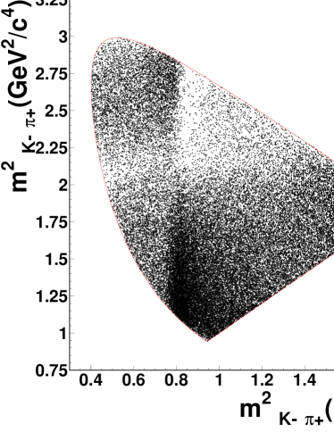
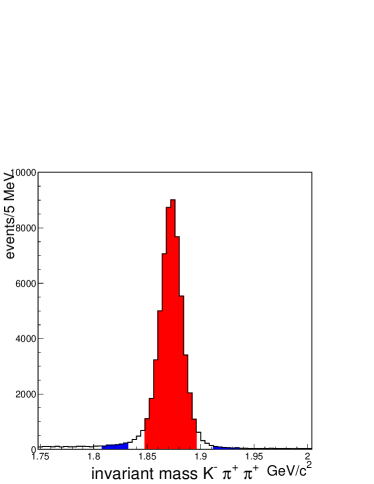
Figure 1: $D^{+}\to K^{-}\pi^{+}\pi^{+}$ Dalitz plot and mass distribution: signal and sideband regions are indicated in red and blue respectively. Sideband are at $\pm$(6–8) $\sigma$ from the peak.

3 The Dalitz plot analysis

Previous analyses of the $D^{+}\to K^{-}\pi^{+}\pi^{+}$ used an isobar model, where the decay amplitude consists of a simple sum of Breit–Wigner functions. In this analysis, the masses and widths for scalar states will be determined by fitting to this particular decay channel. This model usefully serves as the standard for quality of fit, with no presumption as to the correctness of the physics the model embodies. The limitation of this approach, as already mentioned, is that the parameters of the scalar states are “ad hoc”, established with no reference to those found in other processes, in particular scattering data. Moreover, the states involved are wide and overlapping and the Breit–Wigner modelling is too simplistic. Assuming dominance of two-body interactions the K-matrix formalism [5, 6] provides the correct treatment for the $S$-wave $K\pi$ system. It is instructive to compare the K-matrix against this more commonly employed isobar fit and we will present and discuss the results for the two approaches. A third approach, namely a partial-wave analysis of the $K\pi\pi$ system, will be considered in a future publication.

3.1 The isobar model

The decay amplitude in this formalism is written as a coherent sum of amplitudes corresponding to a constant term for the uniform direct three-body decay and to different resonant channels:

$$\mathcal{M}=a_{0}e^{i\delta_{0}}+\sum_{j}a_{j}\leavevmode\nobreak\ e^{i\delta_{j}}\leavevmode\nobreak\ B(abc|r),$$ (1)

where $a,b$ and $c$ label the final-state particles. Coefficient and phase of the $K^{*}(892)$, our reference amplitude, are fixed to 1 and 0 respectively.

$B(abc|r)=B(a,b|r)S(a,c)$ where $B(a,b|r)$ is the Breit–Wigner function

$$B(a,b|r)=\frac{F_{D}F_{r}}{M^{2}_{r}-M^{2}_{ab}-i\Gamma M_{r}},$$ (2)

and $S(a,c)=1$ for a spin-0 resonance, $S(a,c)=-2{\bf a}\cdot{\bf c}$ for a spin-1 resonance and $S(a,c)\,=\,2\left(3({\bf a}\cdot{\bf c})^{2}-|a|^{2}|c|^{2}\right)$ for a spin-2 state. The ${\bf a}$ and ${\bf c}$ are the three-momenta of particles $a$ and $c$ measured in the $ab$ rest frame. The momentum-dependent form factors $F_{D}$ and $F_{r}$ represent the strong coupling at each decay vertex, and are of the Blatt–Weisskopf form. For each resonance of mass $M_{r}$ and spin $J$ we use a width

$$\Gamma=\Gamma_{r}\left(\frac{p}{p_{r}}\right)^{2J+1}\frac{M_{r}}{M_{ab}}\,\frac{F^{2}_{r}(p)}{F^{2}_{r}(p_{r})},$$ (3)

where $p$ is the decay three-momentum in the resonance rest frame and the subscript $r$ denotes the on-shell values. The order of particle label is important for defining the phase convention; here the first particle is the opposite-sign one, i.e., the kaon. Each decay amplitude is then Bose-symmetrized with respect to the exchange of the two identical pions.

3.2 The K-matrix model

The model of $S$-wave states requires particular care in order to account for non-trivial dynamics generated by the presence of broad and overlapping resonances: a real K-matrix guarantees unitarity for two-body interactions. An additional complication in the $K\pi$ system comes from the presence in the $S$-wave of the two isospin states, $I=1/2$ and $I=3/2$.

The K-matrix form we use as input describes the $S$-wave $K^{-}\pi^{+}\to K^{-}\pi^{+}$ scattering from the LASS experiment [12] for energy above 825 MeV and $K^{-}\pi^{-}\to K^{-}\pi^{-}$ scattering from Estabrooks et al. [13]. The K-matrix form follows the extrapolation down to $K\pi$ threshold for both $I=1/2$ and $I=3/2$ $S$-wave components by the dispersive analysis by Büttiker et al. [14], consistent with Chiral Perturbation Theory [15]. The complete form is given below in Eqs. (7-9) with the parameters listed in Table 1 [16].

Although only the $I=1/2$ is dominated by resonances, both isospin components are involved in the decay of the $D^{+}$ meson into $K^{-}\pi^{+}\pi^{+}$. A model for the decay amplitudes of the two isospin states can be constructed from the 2 $\times$ 2 K-matrix describing the $I=1/2$ $S$-wave scattering in $(K\pi)_{1}$ and $(K\eta^{\prime})_{2}$ (with the subscripts 1 and 2, respectively, labelling these two channels), and the single-channel K-matrix describing the $I=3/2$ $K^{-}\pi^{+}\to K^{-}\pi^{+}$ scattering.

The total $D$ decay amplitude in Eq. (1) can be written as

$$\mathcal{M}={(F_{1/2})}_{1}(s)+F_{3/2}(s)+\sum_{j}a_{j}\leavevmode\nobreak\ e^{i\delta_{j}}\leavevmode\nobreak\ B(abc|r),$$ (4)

where $s=M^{2}(K\pi)$, ${(F_{1/2})}_{1}$ and $F_{3/2}$ represent the $I=1/2$ and $I=3/2$ decay amplitudes in the $K\pi$ channel, $j$ runs over vector and spin-2 tensor resonances , and $\leavevmode\nobreak\ B(abc|r)$ are Breit–Wigner forms as in Eq. (1) and Eq. (2). The $J>0$ resonances should, in principle, be treated in the same K-matrix formalism. However, the contribution from the vector wave comes mainly from the $K^{*}(892)$ state, which is well separated from the higher mass $K^{*}(1410)$ and $K^{*}(1680)$, and the contribution from the spin-2 wave comes from $K_{2}^{*}(1430)$ alone. Their contributions are limited to small percentages, and, as a first approximation, they can be reasonably described by a simple sum of Breit–Wigners. More precise results would require a better treatment of the overlapping $K^{*}(1410)$ and $K^{*}(1680)$ resonances as well. $F_{1/2}$ is actually a vector consisting of two components: the first accounting for the description of the $K\pi$ channel, the second of the $K\eta^{\prime}$ channel: in fitting $D^{+}\to K^{-}\pi^{+}\pi^{+}$ we need, of course, the ${(F_{1/2})}_{1}$ element. Its form is

$$(F_{1/2})_{1}=(I-iK_{1/2}\rho)_{1j}^{-1}(P_{1/2})_{j},$$ (5)

where $I$ is the identity matrix, $K_{1/2}$ is the K-matrix for the $I=1/2$ $S$-wave scattering in $K\pi$ and $K\eta^{\prime}$, $\rho$ is the corresponding phase-space matrix for the two channels [6] and $(P_{1/2})_{j}$ is the production vector in the channel $j$. In this model [7], the production process can be viewed as consisting of an initial preparation of states, described by the P-vector, which then propagates according to $(I-iK\rho)^{-1}$ into the final one.

The form for $F_{3/2}$ is

$$F_{3/2}=(I-iK_{3/2}\rho)^{-1}P_{3/2},$$ (6)

where $K_{3/2}$ is the single-channel scalar function describing the $I=3/2$   $K^{-}\pi^{+}\to K^{-}\pi^{+}$ scattering, and $P_{3/2}$ is the production function into $K\pi$.

The $K_{I}$ matrix for the isospin $I$ state is derived by fitting scattering data via the corresponding $\mathcal{T}_{I}$ matrix defined as

$$\mbox{$\mathcal{T}_{I}=(I-iK_{I}\rho)^{-1}K_{I}$}.$$ (7)

The ($\mathcal{T}_{1/2})_{11}$ and $\mathcal{T}_{3/2}$ functions are composed to fit the $K^{-}\pi^{+}\to K^{-}\pi^{+}$ $S$-wave through the Clebsch–Gordan coefficients to give $\mathcal{T}_{11}=(\mathcal{T}_{1/2})_{11}+\mathcal{T}_{3/2}/2$.

Fitting of the real and imaginary parts of the $K^{-}\pi^{+}\to K^{-}\pi^{+}$ LASS amplitude, shown in Fig. 2, and using the predictions of Chiral Perturbation Theory to continue this to threshold, gives the K-matrix parameters in Table 1.

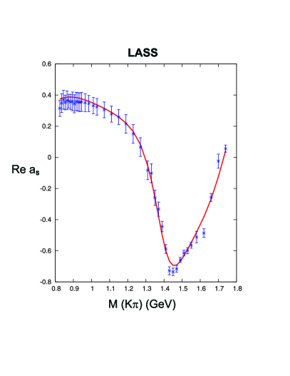
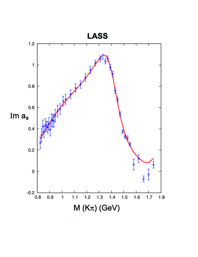
Figure 2: Real and imaginary $K^{-}\pi^{+}\to K^{-}\pi^{+}$ amplitudes from the LASS experiment and their K-matrix fit results.

The $I=1/2$ K-matrix is a one-pole, two-channel matrix whose elements are given in Eq. (3.2).

$$K_{11} = \left(\frac{s-s_{0\frac{1}{2}}}{s_{\text{norm}}}\right)\left(\frac{g_{1}\cdot g_{1}}{s_{1}-s}+C_{110}+C_{111}\tilde{s}+C_{112}\tilde{s}^{2}\right)$$

$$K_{22} = \left(\frac{s-s_{0\frac{1}{2}}}{s_{\text{norm}}}\right)\left(\frac{g_{2}\cdot g_{2}}{s_{1}-s}+C_{220}+C_{221}\tilde{s}+C_{222}\tilde{s}^{2}\right)$$

$$K_{12} = \left(\frac{s-s_{0\frac{1}{2}}}{s_{\text{norm}}}\right)\left(\frac{g_{1}\cdot g_{2}}{s_{1}-s}+C_{120}+C_{121}\tilde{s}+C_{122}\tilde{s}^{2}\right),$$ (8)

where the factor of $s_{norm}=m_{K}^{2}+m_{\pi}^{2}$ is conveniently introduced to make the individual terms in the above expression dimensionless. $g_{1}$ and $g_{2}$ are the real couplings of the $s_{1}$ pole to the first and the second channel respectively. $s_{0\frac{1}{2}}=0.23$ GeV² is the Adler zero position in the $I=1/2$ ChPT elastic scattering amplitude . $C_{11i}$, $C_{22i}$ and $C_{12i}$ for $i=0,1,2$ are the three coefficients of a second order polynomial for the diagonal and off-diagonal elements of the symmetric K-matrix. Polynomials are expanded around $\tilde{s}=s/s_{norm}-1$. This form generates an S-matrix pole, which is conventionally quoted in the complex energy plane as $E=M-i\Gamma/2=1.408-{\it i}0.110$ GeV. Any more distant pole than $K_{0}^{*}(1430)$ is not reliably determined as this simple K-matrix expression does not have the required analyticity properties. Nevertheless, it is an accurate description for real values of the energy where scattering takes place. Numerical values of the terms in Eq. (3.2) are reported in Table 1.

pole (GeV2)	coupling (GeV)	$C_{11i}$	$C_{12i}$	$C_{22i}$
$s_{1}=1.7919$
	$g_{1}=0.31072$
	$g_{2}=-0.02323$
		$C_{110}=0.79299$	$C_{120}=0.15040$	$C_{220}=0.17054$
		$C_{111}=-0.15099$	$C_{121}=-0.038266$	$C_{221}=-0.0219$
		$C_{112}=0.00811$	$C_{122}=0.0022596$	$C_{222}=0.00085655$

Table 1: Values of parameters for the $I=1/2$ K-matrix.

The $I=3/2$ K-matrix is given in Eq. (9). Its form is derived from a simultaneous fit to LASS data [12] and to $K^{-}\pi^{-}\to K^{-}\pi^{-}$ scattering data [13]. It is a non-resonant, one channel scalar function.

$$K_{3/2}=\left(\frac{s-s_{0\frac{3}{2}}}{s_{\text{norm}}}\right)\left(D_{110}+D_{111}\tilde{s}+D_{112}\tilde{s}^{2}\right).$$ (9)

In Eq. (9) $s_{0\frac{3}{2}}=0.27$ GeV² is the Adler zero position in the $I=3/2$ ChPT elastic scattering and the values of the polynomial coefficients are $D_{110}=-0.22147$, $D_{111}$ = 0.026637, and $D_{112}=-0.00092057$ [16].

When moving from scattering processes to $D$-decays, the production P-vector has to be introduced. While the K-matrix is real, P-vectors are in general complex reflecting the fact that the initial coupling $D^{+}\to(K^{-}\pi^{+})\pi^{+}_{spectator}$ need not be real. The P-vector has to have the same poles as the K-matrix, so that these cancel in the physical decay amplitude. Their functional forms are:

$$(P_{1/2})_{1}=\frac{\beta g_{1}e^{i\theta}}{s_{1}-s}+(c_{10}+c_{11}\widehat{s}+c_{12}{\widehat{s}}^{2})e^{i\gamma_{1}}$$ (10)

$$(P_{1/2})_{2}=\frac{\beta g_{2}e^{i\theta}}{s_{1}-s}+(c_{20}+c_{21}\widehat{s}+c_{22}{\widehat{s}}^{2})e^{i\gamma_{2}}$$ (11)

$$P_{3/2}=(c_{30}+c_{31}\widehat{s}+c_{32}{\widehat{s}}^{2})e^{i\gamma_{3}}.$$ (12)

$\beta e^{i\theta}$ is the complex coupling to the pole in the ‘initial’ production process, $g_{1}$ and $g_{2}$ are the couplings as given by Table 1. The $K\pi$ mass squared $s_{c}=2$ GeV² corresponds to the centre of the Dalitz plot. It is convenient to choose this as the value of $s$ about which the polynomials of Eqs. (10-12) are expanded, by defining $\widehat{s}=s-s_{c}$. The polynomial terms in each channel are chosen to have a common phase $\gamma_{i}$ to limit the number of free parameters in the fit and avoid uncontrolled interference among the physical background terms. Thus the coefficients of the second order polynomial, $c_{ij}$, are real. Coefficients and phases of the P-vectors, except $g_{1}$ and $g_{2}$, are the only free parameters of the fit determining the scalar components.

3.3 The likelihood function and fitting procedure

In analogy with our previous works we perform a fit to the $D^{+}$ Dalitz plot with an unbinned likelihood function, $\mathcal{L}$, consisting of signal and background probability density. The signal probability density is corrected for geometrical acceptance and reconstruction efficiency. The shape of the background in the signal region is fixed to that derived from a fit to the Dalitz plot of the mass sidebands. It is parametrized through an incoherent sum of a polynomial function plus resonant Breit–Wigner-like components. The signal fraction is estimated by a fit to the $K^{-}\pi^{+}\pi^{+}$ mass spectrum. Checks for fitting procedure are made using Monte Carlo techniques and all biases are found to be small compared to the statistical errors. The systematic errors on our results include split-sample and fit-variant components [1, 17]. The sample is split in three different ways: low and high $D$ momenta, $D^{+}$ and $D^{-}$, and according to the two main running periods of the experiment.
The fit-variant systematics is evaluated by varying the background parametrization used to fit the sideband Dalitz plot, moving the sideband regions, and letting the background freely float within the error returned by the sideband fit.

3.4 Isobar model results

We allow for the possibility of contributions from all known well-established ($K^{-}\pi^{+}$) resonances[18]. In addition, a constant amplitude accounts for the direct decay of the $D$ meson into a non-resonant three-body final states. The fit parameters are amplitude coefficients $a_{i}$ and phases $\delta_{i}$ of Eq. (1). Contributions are removed if their amplitude coefficients, $a_{i}$ have less than $2\,\sigma$ significance and the fit confidence level increases. The fit confidence levels (C.L.) are evaluated with a $\chi^{2}$ estimator over the Dalitz plot with bin size adaptively chosen to maintain a minimum number of events in each bin. A fit consisting solely of well-established $K^{-}\pi^{+}$ resonances with masses and widths as in the PDG [18] results in a very poor solution, with an adaptive bin $\chi^{2}$/d.o.f of more than 3, and with a very high level of the non-resonant component, about 90% of the total, atypically high for charm decays.

Following a previous work [19] a low mass $K^{-}\pi^{+}$ resonance $\kappa$ is introduced with mass and width freely floating in the fit. The insertion of this state, whose mass and width are fitted to be 883 $\pm$ 13 MeV/c² and 355 $\pm$ 13 MeV/$c^{2}$ respectively, returns a $\chi^{2}$/d.o.f of more than 2. Only a simultaneous redefinition of the Breit–Wigner parameters for the higher-mass scalar $K^{*}_{0}(1430)$ and the inclusion of $\kappa$ gives an acceptable fit with a $\chi^{2}$/d.o.f of 1.17, corresponding to a 6.8% C.L. The mass and width of this effective $K^{*}_{0}(1430)$ are 1461 $\pm$ 4 MeV/c² and 177 $\pm$ 8 MeV/c², respectively; they can be compared to the PDG values of mass 1412 $\pm$ 6 MeV/$c^{2}$ and width 294 $\pm$ 23 MeV/$c^{2}$, and to the K-matrix fit values of mass 1408 MeV/$c^{2}$ and width 220 MeV/$c^{2}$. The parameters for the $\kappa$ in a fit with a free $K^{*}_{0}(1430)$ are mass 856 $\pm$ 17 MeV/$c^{2}$ and width 464 $\pm$ 28 MeV/$c^{2}$. In Table 2, fit fractions, phases and coefficients of the various amplitudes from the fit are reported, along with masses and widths for $\kappa$ and $K^{*}_{0}(1430)$.

channel	fit fraction (%)	phase $\delta_{i}$ (deg)	coefficient
$non-resonant$	$29.7\pm 4.5$	$325\pm 4$	$1.47\pm 0.11$
	$\pm\ 1.5\pm 2.1$ (see text)	$\pm\ 2\pm 1.2$	$\pm\ 0.06\pm 0.06$
$K^{*}(892)\pi^{+}$	$13.7\pm 0.9$	$0$ (fixed)	$1$(fixed)
	$\pm\ 0.6\pm 0.3$
$K^{*}(1410)\pi^{+}$	$0.2\pm 0.1$	$350\pm 34$	$0.12\pm 0.03$
	$\pm\ 0.1\pm 0.04$	$\pm\ 17\pm 15$	$\pm\ 0.003\pm 0.01$
$K^{*}(1680)\pi^{+}$	$1.8\pm 0.4$	$3\pm 7$	$0.36\pm 0.04$
	$\pm\ 0.2\pm 0.3$	$\pm\ 4\pm 8$	$\pm\ 0.02\pm 0.03$
$K^{*}_{2}(1430)\pi^{+}$	$0.4\pm 0.05$	$319\pm 8$	$0.17\pm 0.01$
	$\pm\ 0.04\pm 0.03$	$\pm\ 2\pm 2$	$\pm\ 0.01\pm 0.01$
$K^{*}_{0}(1430)\pi^{+}$	$17.5\pm 1.5$	$36\pm 5$	$1.13\pm 0.05$
	$\pm\ 0.8\pm 0.4$	$\pm\ 2\pm 1.2$	$\pm\ 0.01\pm 0.02$
$\kappa\pi^{+}$	$22.4\pm 3.7$	$199\pm 6$	$1.28\pm 0.10$
	$\pm\ 1.2\pm 1.5$ (see text)	$\pm\ 1\pm 5$	$\pm\ 0.015\pm 0.04$
	mass (MeV/$c^{2}$)	width (MeV/$c^{2}$)
$K^{*}_{0}(1430)$	$1461\pm 4\pm 2\pm 0.5$	$177\pm 8\pm 3\pm 1.5$
$\kappa$	$856\pm 17\pm 5\pm 12$	$464\pm 28\pm 6\pm 21$

Table 2: Fit fractions, phases, and coefficients from the isobar fit to the FOCUS $D^{+}\to K^{-}\pi^{+}\pi^{+}$ data. The first error is statistic, the second error is systematic from the experiment, and the third error is systematic induced by model input parameters for higher resonances.

Coefficients refer to Bose-symmetrized, normalized amplitudes, both for resonant and non-resonant states. Masses and widths can be compared with previous determinations from E791 [19] and BES [20]. All the results are consistent within the errors. Two systematic uncertainties are quoted in Table 2 : the first includes our split sample and fit variant components of Section 3.3, the second reflects uncertainties due to higher resonance modeling. In particular, this analysis is performed with a fixed radius of 5 GeV^-1 and 1.5 GeV^-1 in the Blatt–Weisskopf $D$-meson and resonance form factors, respectively [19]. To cover the large range of uncertainties we found in literature on these parameters, we estimated the systematic effect by varying them. Furthermore, for $J>0$ resonances we assumed central values for masses and widths from the PDG [18]. For those parameters which are not accurately determined we allowed a $\pm 1\,\sigma$ variation and estimated the systematic uncertainty by the corresponding spread in the results. An analogous study is performed for the K-matrix fit and the corresponding uncertainties are quoted in Table 3 and 4.

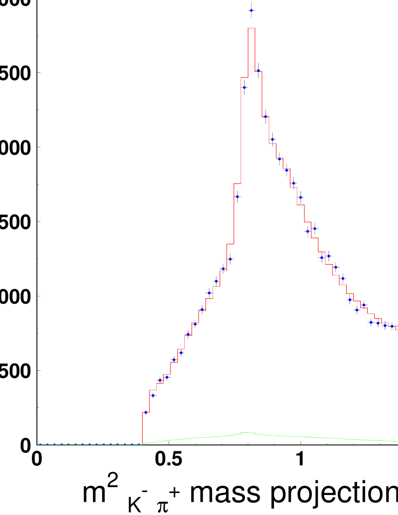
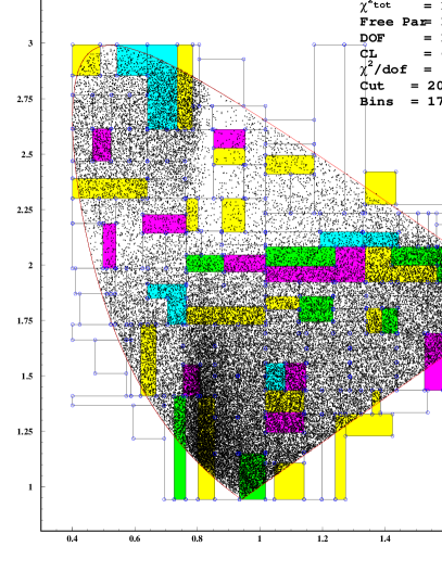
Figure 3: Top: Dalitz plot projections with our isobar fit superimposed. The background shape under the signal is also shown. Bottom: The adaptive binning scheme.

Systematics for the $\kappa$ and non-resonant components have a very large dependence on whether or not Gaussian form factors, suggested in [21], are included in the fit. Our systematic uncertainties do not account for the effect introduced by adding form factor for the scalar resonances. There is still some controversy on whether form factors are even needed for these scalars [22]. We find that adding in the Gaussian form factors does not improve our fit quality (3% C.L versus 6.8% C.L.). In this case, our results become consistent, within the errors, with Model C in [19], and changes the $\kappa$ and non-resonant fit fractions to (40.7 $\pm$ 6.2) % and (17.5 $\pm$ 4.1 )% respectively. Dalitz plot projections with fit results and the corresponding adaptive-binning scheme are shown in Fig. 3.

3.5 K-matrix model results

In the K-matrix fit to the $D^{+}\to K^{-}\pi^{+}\pi^{+}$ decay the free parameters are amplitudes and phases ($a_{i}$ and $\delta_{i}$) for vectors and tensors, and the P-vector parameters for scalar contributions. $K\pi$ scattering determines the parameters of the K-matrix elements and these are fixed inputs to this $D$ decay analysis. Table 3 reports our K-matrix fit results. It shows quadratic terms in $(P_{1/2})_{1}$ are significant in fitting data, while in both $(P_{1/2})_{2}$ and $P_{3/2}$ constants are sufficient.

coefficient	phase (deg)
$\beta$ = $3.389\pm 0.152\pm 0.002\pm 0.068$	$\theta=286\pm 4\pm 0.3\pm 3.0$
$c_{10}$ = $1.655\pm 0.156\pm 0.010\pm 0.101$	$\gamma_{1}=304\pm 6\pm 0.4\pm 5.8$
$c_{11}$ = $0.780\pm 0.096\pm 0.003\pm 0.090$
$c_{12}$ = $-0.954\pm 0.058\pm 0.0015\pm 0.025$
$c_{20}$ = $17.182\pm 1.036\pm 0.023\pm 0.362$	$\gamma_{2}=126\pm 3\pm 0.1\pm 1.2$
$c_{30}$ = $0.734\pm 0.080\pm 0.005\pm 0.030$	$\gamma_{3}=211\pm 10\pm 0.7\pm 7.8$
Total $S$-wave fit fraction = $83.23\pm 1.50\pm 0.04\pm 0.07$ %
Isospin 1/2 fraction = $207.25\pm 25.45\pm 1.81\pm 12.23$ %
Isospin 3/2 fraction = $40.50\pm 9.63\pm 0.55\pm 3.15$ %

Table 3: $S$-wave parameters from the K-matrix fit to the FOCUS $D^{+}\to K^{-}\pi^{+}\pi^{+}$ data. The first error is statistic, the second error is systematic from the experiment, and the third is systematic induced by model input parameters for higher resonances. Coefficients are for the unnormalized $S$-wave.

The $J>0$ states required by the fit are listed in Table 4.

component	fit fraction (%)	phase $\delta_{j}$ (deg)	coefficient
$K^{*}(892)\pi^{+}$	$13.61\pm 0.98$	0 (fixed)	1 (fixed)
	$\pm\ 0.01\pm 0.30$
$K^{*}(1680)\pi^{+}$	$1.90\pm 0.63$	$1\pm 7$	$0.373\pm 0.067$
	$\pm\ 0.009\pm 0.43$	$\pm\ 0.1\pm 6$	$\pm\ 0.009\pm 0.047$
$K^{*}_{2}(1430)\pi^{+}$	$0.39\pm 0.09$	$296\pm 7$	$0.169\pm 0.017$
	$\pm\ 0.004\pm 0.05$	$\pm\ 0.3\pm 1$	$\pm\ 0.010\pm 0.012$
$K^{*}(1410)\pi^{+}$	$0.48\pm 0.21$	$293\pm 17$	$0.188\pm 0.041$
	$\pm\ 0.012\pm 0.17$	$\pm\ 0.4\pm 7$	$\pm\ 0.002\pm 0.030$

Table 4: Fit fractions, phases, and coefficients for the $J>0$ components from the K-matrix fit to the FOCUS $D^{+}\to K^{-}\pi^{+}\pi^{+}$ data. The first error is statistic, the second error is systematic from the experiment, and the third error is systematic induced by model input parameters for higher resonances.

The $S$-wave component accounts for the dominant portion of the decay $(83.23\pm 1.50)\%$, and is the sum of the $I=1/2$ and $I=3/2$ components, which, separately, account for the (207 $\pm$ 24)% and (40 $\pm$ 9)% of the decay, with $-164$ % from their interference. The large amount of interference between the $I=3/2$ component and the $I=1/2$ component underscores its importance in our K-matrix fit. Because there are no $I=3/2$ resonances, the $I=3/2$ $S$-wave component has at most a slowly varying phase and amplitude and since we find little variation in the $F_{3/2}$-vector phase as well, the $I=3/2$ piece essentially plays a comparable role to the $\sim$ 30% non-resonant component present in the isobar fit summarized by Table 2. A significant fraction, $13.61\pm 0.98$%, comes, as expected, from $K^{*}(892)$; smaller contributions come from two vectors $K^{*}(1410)$ and $K^{*}(1680)$ and from the tensor $K_{2}^{*}(1430)$. It is conventional to quote fit fractions for each component and this is what we do. Care should be taken in interpreting some of these since strong interference can occur. This is particularly apparent between contributions in the same-spin partial wave. While the total $S$-wave fraction is a sensitive measure of its contribution to the Dalitz plot, the separate fit fractions for $I=1/2$ and $I=3/2$ must be treated with care. The broad $I=1/2$ $S$-wave component inevitably interferes strongly with the slowly varying $I=3/2$ $S$-wave, as seen for instance in [23]. Fit results on the projections and the adaptive binning scheme are shown in Fig. 4.

The fit $\chi^{2}$/d.o.f is 1.27 corresponding to a confidence level of 1.2%. If the $I=3/2$ component is removed from the fit, the $\chi^{2}$/d.o.f worsens to 1.54, corresponding to a confidence level of $10^{-5}$.

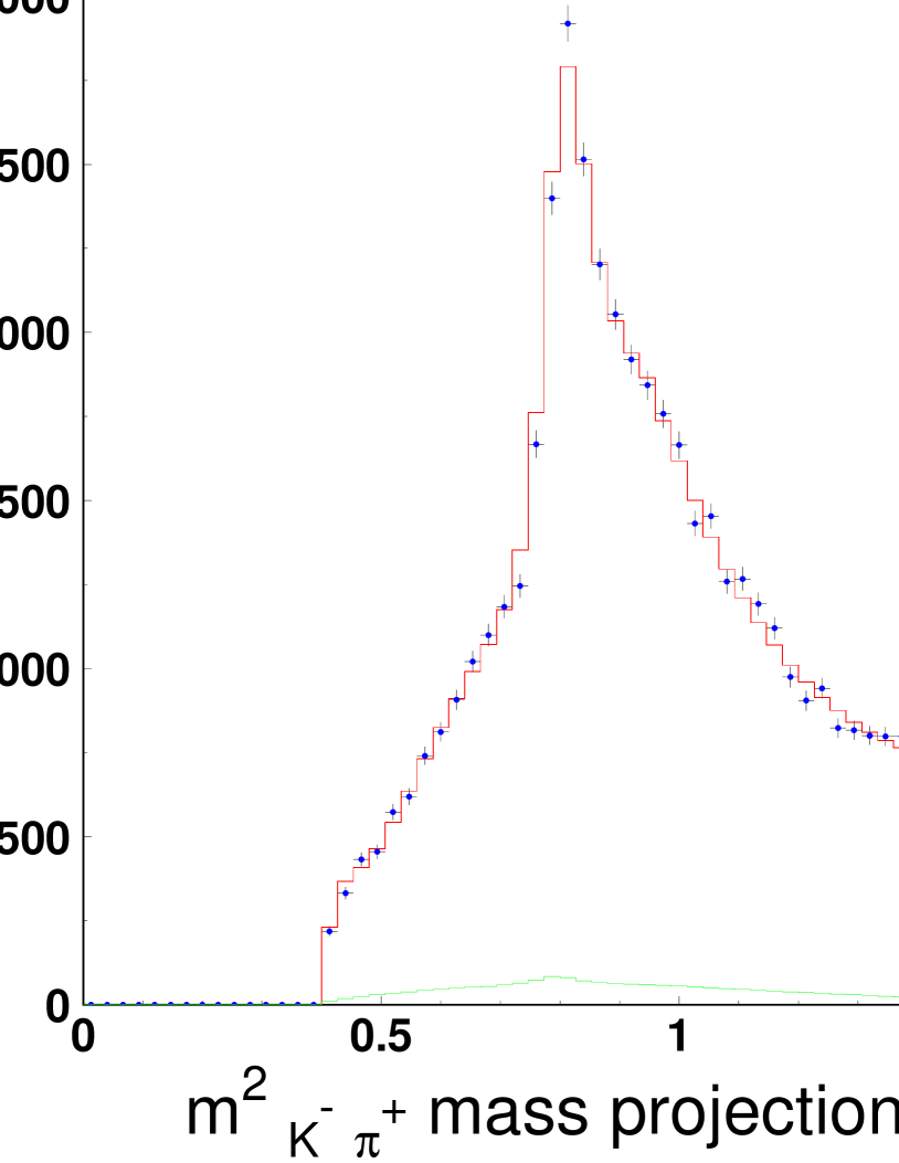
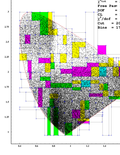
Figure 4: Top: The Dalitz plot projections with the K-matrix fit superimposed. The background shape under the signal is also shown. Bottom: The adaptive binning scheme.

3.6 Comparison and discussion of the results

The isobar fit represents a good effective description of the data, as testified by the confidence level. However, simple Breit–Wigner forms have been used for both the broad scalars $\kappa$ and $K^{*}_{0}(1430)$, each with free mass and width with no reference to how these states appear in other $K\pi$ interactions. Elastic scattering provides independent information about these states, their shape and parameters and how they overlap. In particular, scattering data from LASS show that the phase of the $S$-wave rises by no more than $100^{\circ}$ from 825 to 1450 MeV, while the isobar fit with its simple Breit–Wigner forms requires $\sim 180^{\circ}$ change in the resonant $I=1/2$ $S$-wave. In Fig. 5a) and b) we compare the modulus and phase of the total $S$-wave components from the isobar and K-matrix fits. They essentially agree, as expected, since they fit the same data. However, the physics description differs considerably in the $I=1/2$ components. In Fig. 5 c) and d) modulus and phase of the $I=1/2$ $S$-wave component from our K-matrix fit are shown.

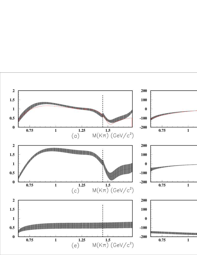
Figure 5: Modulus and phase of the $S$-wave components resulting from the K-matrix and isobar fit. Bands represent the $\pm 1\,\,\sigma$ statistical variation of the K-matrix results for the total component [ a) and b) plots], the $I=1/2$ component [ c) and d) plots)] and the the $I=3/2$ component [ e) and f)] plots). Continuous lines in a) and b) represent the central value of the isobar fit. Vertical dashed line shows the location of the $K\eta^{\prime}$ threshold.

The motivation for the K-matrix fit was to bring consistency between the description of scattering and $D$-decay data. In such a formalism the poles of the $S$-matrix are process independent, and on the real energy axis the overlap of broad resonances is correctly described. The results of the K-matrix fit showed that such a consistent representation is equally possible, the global fit quality being indeed good. However, it deteriorates at higher $K\pi$ mass. This is not surprising since our K-matrix treatment only includes two channels $K\pi$ and $K\eta^{\prime}$. While we have reliable information on the former channel, we have relatively poor constraints on the latter. This means that as we consider $K\pi$ masses far above $K\eta^{\prime}$ threshold, these inadequacies in the description of the $K\eta^{\prime}$ channel become increasingly important. This is expected to become worse as yet further inelastic channels open up. Consequently, improvements could be made by using a number of $D$-decay chains with $K\pi$ final state interactions and inputting all these in one combined analysis in which several inelastic channels are included in the K-matrix formalism. In the present single $D^{+}\to K^{-}\pi^{+}\pi^{+}$ channel, adding further inelastic modes would be just adding free unconstrained parameters for which there is little justification. It is interesting to note that the adaptive binning scheme shows that both the K-matrix and the isobar fit are not able to reproduce data well in the region at 2 GeV², in the vicinity of the $K\eta^{\prime}$ threshold. It is also the energy domain where higher spin states live. Vector and tensor fit parameters in the two models are in very good agreement: we do not exclude the possibility that a better treatment of these amplitudes could improve the $\chi^{2}$. Some isolated spots of high $\chi^{2}$ could be caused by an imperfect modeling of the efficiency as they are in the same regions in both fits. The FOCUS experiment has also studied the $K^{-}\pi^{+}$ amplitudes in the $D^{+}\to K^{-}K^{+}\pi^{+}$ decay. We note that the moduli of Fig. 5a) are very different than that presented in Fig. 3a) of [24]. This underscores the fact that different decay modes of the same charm state can often have quite different shapes for the moduli of their amplitudes, reflecting the differing production dynamics encoded in the P-vectors.

4 Conclusions

The analysis of the $D^{+}\to K^{-}\pi^{+}\pi^{+}$ decay with the two models described in this paper reveal quite different features. The isobar model with its Breit–Wigner representation for all states requires both a $\kappa$ and a $K^{*}_{0}(1430)$ whose parameters are not what elastic scattering would require. However, as already indicated, such Breit–Wigner parameters are effective rather than genuine pole positions. In contrast, the K-matrix fit has built in consistency with $K\pi$ scattering. Moreover, this agrees with the results of our FOCUS experiment in semi-leptonic $D$-decay [25, 26, 27], where we have shown that the $S$-wave phase agrees with that of the LASS experiment. The hypothesis of the two-body dominance, which has already been tested in other charm meson decays, is consistent with our results for the high-statistics $D^{+}\to K^{-}\pi^{+}\pi^{+}$. Previous analyses [28] did not allow for the two different isospin states, and compared the $I=1/2$ scattering phase with the global scalar phase. Comparison with our global F-vector phase is shown in the left plot of Fig. 6.

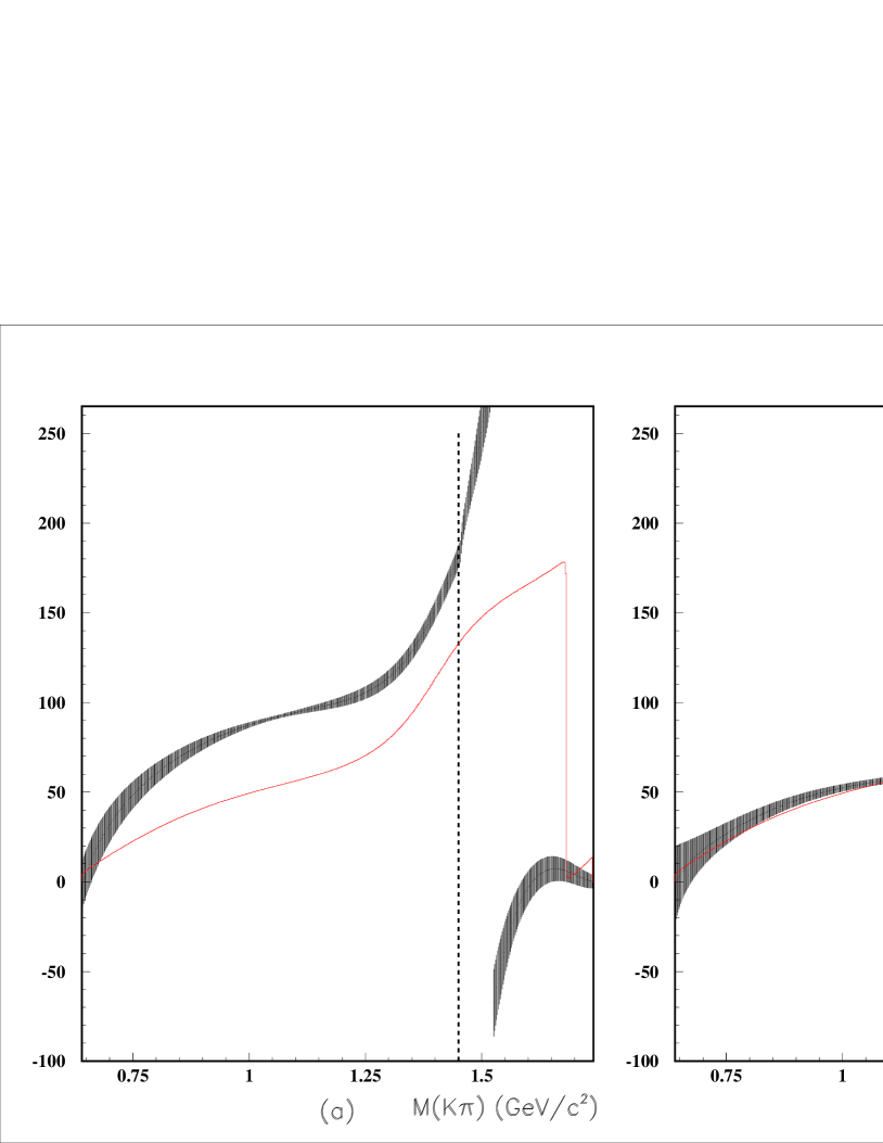
Figure 6: Comparison between the LASS $I=1/2$ phase + ChPT (continous line) and the F-vector phases (with $\pm 1\,\sigma$ statical error bars); a) total F-vector phase; b) $I=1/2$ F-vector phase. Vertical dashed line shows the location of the $K\eta^{\prime}$.

A feature of the K-matrix amplitude analysis is that it allows an indirect phase measurement of the separate isospin components: it is this phase variation with isospin $I=1/2$ which should be compared with the same $I=1/2$ LASS phase, extrapolated from 825 GeV down to threshold according to Chiral Perturbation Theory. This is done in the right plot of Fig. 6. As explained in Section 3.2, in this model [7] the P-vector allows for a phase variation accounting for the interaction with the third particle in the process of resonance formation. It so happens that the Dalitz fit gives a nearly constant production phase. The two phases in Fig. 6b) have the same behaviour up to $\sim$ 1.1 GeV. However, approaching $K\eta^{\prime}$ threshold, effects of inelasticity and differing final state interactions start to appear. The difference between the phases in Fig. 6a) is due to the $I=3/2$ component.

These results are consistent with $K\pi$ scattering data, and consequently with Watson’s theorem predictions for two-body $K\pi$ interactions in the low $K\pi$ mass region, up to $\sim$ 1.1 GeV, where elastic processes dominate. This means that possible three-body interaction effects, not accounted for in the K-matrix parametrization, play a marginal role.

Our results for the total $S$-wave are in general agreement with those from the E791 analysis, in which the $S$-wave modulus and phase were determined in each $K\pi$ slice [28], [29]. Edera and Pennington [23] were able to separate this total $S$-wave into $I=1/2$ and $I=3/2$ components, making the strong assumption that the equivalent of the P-vector has a constant phase. Here we have relaxed this assumption, and find a slightly different separation of $I=1/2$ and $3/2$ components, but the trend with energy and relative phases are broadly consistent.

What does this analysis contribute to the discussion of the existence and parameters of the $\kappa$? We know from analysis [30] of the LASS data (which in $K^{-}\pi^{+}$ scattering only start at 825 MeV) there is no pole, the $\kappa(900)$, in its energy range. However, below 800 MeV, deep in the complex plane, there is very likely such a state. Its precise location requires a more sophisticated analytic continuation onto the unphysical sheet than the K-matrix representation provided here. This is because of the need to approach close to the crossed channel cut, which is not correctly represented for a robust analytic continuation. However, our K-matrix representation fits along the real energy axis inputs on scattering data and Chiral Perturbation Theory in close agreement with those used in the analysis by Descotes-Genon and Moussallam [31] that locates the $\kappa$ with a mass of $(658\pm 13)$ MeV and a width of $(557\pm 24)$ MeV by careful continuation. These pole parameters are quite different from those implied by the simple isobar fits presented here, and by E791 in [19]. What we have shown is that whatever $\kappa$ is revealed by our $D^{+}\to K^{-}\pi^{+}\pi^{+}$ results, it is the same as that found in scattering data. Consequently, our analysis supports the conclusions of [31] and [32].

We have seen that $D$-decay can teach us about $K\pi$ interaction much closer to threshold than the older scattering results. This serves as a valuable check from experiment [33] of the inputs to the analyses of [31] and [32] based largely on theoretical considerations. Indeed, more complete experimental insight into the $K\pi$ interaction will be provided by the full range of hadronic and semi-leptonic $D$-decays to come from $B$-factories. Our results show that the dynamics of the $K^{-}\pi^{+}\pi^{+}$ final state is dominated by two-body $K\pi$ interactions up to 1.1 GeV as determined by scattering experiments.

5 Acknowledgments

We wish to acknowledge the assistance of the staffs of Fermi National Accelerator Laboratory, the INFN of Italy, and the physics departments of the collaborating institutions. This research was supported in part by the U. S. National Science Fundation, the U. S. Department of Energy, the Italian Istituto Nazionale di Fisica Nucleare and Ministero dell’Università e della Ricerca Scientifica e Tecnologica, the Brazilian Conselho Nacional de Desenvolvimento Científico e Tecnológico, CONACyT-México, the Korean Ministry of Education, and the Korean Science and Engineering Foundation.

References

- [1] J. M. Link et al., Phys. Lett. B585 (2004) 200.
- [2] I. Caprini, G. Colangelo and H. Leutwyler, Phys. Rev. Lett. 96 (2006) 132001.
- [3] D. V. Bugg, Eur. Phys. J. C37 (2004) 433.
- [4] J. A. Oller, Phys. Rev. D71 (2005) 05404030.
- [5] E. P. Wigner, Phys. Rev. 70 (1946) 15.
- [6] S. U. Chung et al., Annalen Phys. 4 (1995) 404.
- [7] I. J. R. Aitchison, Nucl. Phys. A189, (1972) 417.
- [8] P. L. Frabetti et al. Nucl. Instrum. Meth. A320 (1992) 519.
- [9] J. M. Link et al., Nucl. Instrum. Meth. A484 (2002) 270.
- [10] J. M. Link et al., Phys. Lett. B485 (2000) 62.
- [11] J. M. Link et al., Phys. Lett. B537 (2002) 192.
- [12] D. Aston et al., Nucl. Phys. B296 (1988) 493.
- [13] P. Estabrooks et al., Nucl. Phys. B133 (1978) 490.
- [14] P. Büttiker, S. Descotes-Genon and B. Moussallam, Nucl. Phys. Proc. Suppl. 133 (2004) 223; Eur. Phys. J. C33 (2004) 409.
- [15] V. Bernard, N. Kaiser and U. G. Meißner, Phys. Rev. D43 (1991) 2757; Nucl. Phys. B357 (1991) 129.
- [16] M. R. Pennington, private communication.
- [17] J. M. Link et al., Phys. Lett. B601 (2004) 10.
- [18] Particle Data Group, J. Phys. G: Nucl. Part. Phys. 33 (2006) 1
- [19] E. M. Aitala et al., Phys. Rev. Lett. 89 (2002) 121801.
- [20] M. Ablikim et al., Phys. Lett. B633 (2006) 681.
- [21] N. A. Tőrnqvist, Z. Phys. C68 (1995) 647.
- [22] D. V. Bugg, Phys. Lett. B632 (2006) 471.
- [23] L. Edera, M. R. Pennington, Phys. Lett. B623 (2005) 55.
- [24] J. M. Link et al., Phys. Lett. B648 (2007) 156.
- [25] J. M. Link et al., Phys. Lett. B535 (2002) 43.
- [26] J. M. Link et al., Phys. Lett. B544 (2002) 89.
- [27] J. M. Link et al., Phys. Lett. B621 (2005) 72.
- [28] E. M. Aitala et al., Phys. Rev. D73 (2006) 032004.
- [29] M. R. Pennington, Int. J. Mod. Phys. A21 (2006) 5503.
- [30] S. N. Cherry and M. R. Pennington, Nucl. Phys. A688 (2001) 823.
- [31] S. Descotes-Genon and B. Moussallam, Eur. Phys. J. C48 (2006) 553.
- [32] Z.Y. Zhou and H.Q. Zheng, Nucl. Phys. A775 (2006) 212.
- [33] S. Malvezzi and M. R. Pennington (in preparation).