Wightman function and vacuum densities for a $Z_{2}$-symmetric thick brane in AdS spacetime

Abstract

Positive frequency Wightman function, vacuum expectation values of the field square and the energy-momentum tensor induced by a $Z_{2}$-symmetric brane with finite thickness located on $(D+1)$- dimensional AdS background are evaluated for a massive scalar field with general curvature coupling parameter. For the general case of static plane symmetric interior structure the expectation values in the region outside the brane are presented as the sum of free AdS and brane induced parts. For a conformally coupled massless scalar the brane induced part in the vacuum energy-momentum tensor vanishes. In the limit of strong gravitational fields the brane induced parts are exponentially suppressed for points not too close to the brane boundary. As an application of general results a special model is considered in which the geometry inside the brane is a slice of the Minkowski spacetime orbifolded along the direction perpendicular to the brane. For this model the Wightman function, vacuum expectation values of the field square and the energy-momentum tensor inside the brane are evaluated as well and their behavior is discussed in various asymptotic regions of the parameters. It is shown that for both minimally and conformally coupled scalar fields the interior vacuum forces acting on the brane boundaries tend to decrease the brane thickness.

PACS: 04.62.+v; 11.10.Kk

1 Introduction

Recent proposals of large extra dimensions use the concept of brane as a sub-manifold embedded in a higher dimensional spacetime, on which the Standard Model particles are confined (see, for instance [1]). Braneworlds naturally appear in string/M-theory context and provide a novel setting for discussing phenomenological and cosmological issues related to extra dimensions. The models introduced by Randall and Sundrum are particularly attractive. In RS 2-brane model [2] the corresponding background solution consists of two parallel flat 3-branes, one with positive tension and another with negative tension embedded in a five dimensional AdS bulk. The fifth coordinate is compactified on $S^{1}/Z_{2}$, and the branes are on the two fixed points. It is assumed that all matter fields are confined on the branes and only the gravity propagates freely in the five dimensional bulk. In RS 1-brane model [3] there is only one positive tension brane in a five dimensional AdS bulk. This model is obtained from 2-brane one by sending the negative tension brane to infinity. Due to the warp factor in the AdS metric the infinite extra dimension gives a finite contribution to the volume. More recently, alternatives to confining particles on the brane have been investigated and scenarios with additional bulk fields have been considered.

Motivated by the problems of the radion stabilization and the generation of cosmological constant, the role of quantum effects in braneworlds has attracted great deal of attention [4]-[42]. A class of higher dimensional models with compact internal spaces is considered in [43]. Many of treatments of quantum fields in braneworlds deal mainly with the case of the idealized brane with zero thickness. This simplification suffers from the disatvantage that the curvature tensor is singular at the brane location. In addition, the vacuum expectation values of the local physical observables diverge on the brane. From a more realistic point of view we expect that the branes have a finite thickness and the thickness can act as natural regulator for surface divergences. The finite core effects also lead to the modification of the Friedmann equation describing the cosmological evolution inside the brane. In particular, a phase with accelerated expansion on the brane can be obtained in the model with pressureless matter as the only non-gravitational source in the modified Friedmann equation. In sting theory there exists the minimum length scale and we cannot neglect the thickness of the corresponding branes at the string scale. The branes modelled by field theoretical domain walls have a characteristic thickness determined by the energy scale where the symmetry of the system is spontaneously broken. Various models are considered for a thick brane (see, for instance, [44] and references therein). Mainly, these models are constructed as solutions to the coupled Einstein-scalar equations by choosing a suitable potential for the scalar field. Vacuum fluctuations for a simple thick de Sitter brane supported by a bulk scalar field with an axion like potential and the self-consistency of this braneworld are investigated in Refs. [40].

In the present paper we investigate the effects of core on properties of the quantum vacuum for the general plane symmetric static model of the brane with finite thickness. The most important quantities characterizing these properties are the vacuum expectation values of the field square and the energy-momentum tensor. Though the corresponding operators are local, due to the global nature of the vacuum, the vacuum expectation values describe the global properties of the bulk and carry an important information about the internal structure of the brane. In addition to describing the physical structure of the quantum field at a given point, the energy-momentum tensor acts as the source of gravity in the Einstein equations. It therefore plays an important role in modelling a self-consistent dynamics involving the gravitational field. As the first step for the investigation of vacuum densities we evaluate the positive frequency Wightman function for a massive scalar field with general curvature coupling parameter. This function gives comprehensive insight into vacuum fluctuations and determines the response of a particle detector of the Unruh-DeWitt type moving in the brane bulk. The problem under consideration is also of separate interest as an example with gravitational and boundary-induced polarizations of the vacuum, where all calculations can be performed in a closed form. The corresponding results specify the conditions under which we can ignore the details of the interior structure and approximate the effect of the brane by the idealized model. In addition, as it will be shown below, the phenomenological parameters in the zero-thickness brane models such as brane mass terms for scalar fields are calculable in terms of the inner structure of the brane within the framework of the model considered in the present paper.

The plan of this paper is as follows. In Section 2 we consider the Wightman function in the exterior of the brane for the general structure of the core assuming that the components of the metric tensor and their derivatives are continuous at the transition surface between the core and the exterior. The Section 3 is devoted to the generalization of the corresponding results when an additional surface shell is present on the bounding surfaces between the core and the exterior. By using the formulae for the Wightman function, in Section 4 we investigate the vacuum expectation values of the field square and the energy-momentum tensor. As an illustration of the general results, in Section 5 we consider a model with Minkowskian geometry inside the brane. For this model the vacuum expectation values inside the core are investigated as well. The last section contains a summary of the work.

2 Wightman function

2.1 Model

We consider a domain wall with finite thickness on background of $(D+1)$-dimensional AdS spacetime. As in RS 1-brane scenario we will assume that our model is $Z_{2}$-symmetric with respect to the plane $y=0$ located at the center of the brane. The spacetime is described by two distinct metric tensors in the regions outside and inside the brane. The corresponding line element in the exterior region $|y|>a$ has the form

$$ds^{2}=g_{ik}dx^{i}dx^{k}=e^{-2k_{D}|y|}\eta_{\mu\nu}dx^{\mu}dx^{\nu}-dy^{2},$$ (2.1)

where $\eta_{\mu\nu}=\mathrm{diag}(1,-1,\ldots,-1)$ is the metric for the $D$-dimensional Minkowski spacetime, $1/k_{D}$ is the AdS curvature radius. Here and below $i,k=0,1,\ldots,D$, and $\mu,\nu=0,1,\ldots,D-1$. We will assume that inside the brane (region $|y|<a$) the spacetime geometry is regular and is described by the static plane symmetric line element

$$ds^{2}=e^{2u(y)}dt^{2}-e^{2v(y)}d\mathbf{x}^{2}-e^{2w(y)}dy^{2},$$ (2.2)

where $\mathbf{x}=(x^{1},\ldots,x^{D-1})$ are coordinates parallel to the brane. Due to the $Z_{2}$-symmetry the functions $u(y)$, $v(y)$, $w(y)$ are even functions on $y$. These functions are continuous at the core boundary:

$$u(a)=v(a)=-k_{D}a,\;w(a)=0.$$ (2.3)

Here we assume that there is no surface energy-momentum tensor located at $|y|=a$ and, hence, the derivatives of these functions are continuous as well. The generalization to the case with an infinitely thin shell at the boundary of two metrics will be discussed in the next section.

For the metric corresponding to line element (2.2) the nonzero components of the Ricci tensor are given by expressions (no summation over $i$)

$$R_{0}^{0} = -e^{-2w}\left[u^{\prime\prime}+u^{\prime 2}+(D-1)u^{\prime}v^{\prime}-u^{\prime}w^{\prime}\right],$$

$$R_{i}^{i} = -e^{-2w}\left[v^{\prime\prime}+(D-1)v^{\prime 2}+v^{\prime}u^{\prime}-v^{\prime}w^{\prime}\right],\;i=1,\ldots,D-1,$$ (2.4)

$$R_{D}^{D} = -e^{-2w}\left[u^{\prime\prime}+(D-1)v^{\prime\prime}+u^{\prime 2}+(D-1)v^{\prime 2}-w^{\prime}u^{\prime}-(D-1)w^{\prime}v^{\prime}\right],$$

where the prime means the derivative with respect to the coordinate $y$. The corresponding Ricci scalar has the form

$$R = -2e^{-2w}\left[u^{\prime\prime}+(D-1)v^{\prime\prime}+u^{\prime 2}+D(D-1)v^{\prime 2}/2\right.$$ (2.5)

$$\left.+(D-1)u^{\prime}v^{\prime}-u^{\prime}w^{\prime}-(D-1)v^{\prime}w^{\prime}\right].$$

In the special case $u(y)=v(y)$ one has $R_{0}^{0}=R_{i}^{i}$, $i=1,\ldots,D-1$, and the model is Poincare invariant along the directions parallel to the brane.

2.2 Eigenfunctions

In this paper we are interested in the vacuum polarization effects for a scalar field with general curvature coupling parameter $\xi$ propagating in the bulk described above. The corresponding field equation has the form

$$\left(\nabla_{i}\nabla^{i}+m^{2}+\xi R\right)\varphi=0,\;\nabla_{i}\nabla^{i}=\frac{1}{\sqrt{|g|}}\partial_{i}(g^{ik}\sqrt{|g|}\partial_{k}),$$ (2.6)

where $\nabla_{i}$ is the covariant derivative operator associated with line element (2.1) outside the brane and with line element (2.2) inside the brane. The values of the curvature coupling parameter $\xi=0$ and $\xi=\xi_{D}$ with $\xi_{D}\equiv(D-1)/4D$ correspond to the most important special cases of minimally and conformally coupled scalar fields. As a first stage for the evaluation of the vacuum expectation values (VEVs) for the field square and the energy-momentum tensor we consider the positive frequency Wightman function $\langle 0|\varphi(x)\varphi(x^{\prime})|0\rangle$, where $|0\rangle$ is the amplitude for the corresponding vacuum state. This function also determines the response of the Unruh-DeWitt type particle detector at a given state of motion (see, for instance, [45]). The Wightman function can be evaluated by using the mode sum formula

$$\langle 0|\varphi(x)\varphi(x^{\prime})|0\rangle=\sum_{\alpha}\varphi_{\alpha}(x)\varphi_{\alpha}^{\ast}(x^{\prime}),$$ (2.7)

where $\left\{\varphi_{\alpha}(x),\varphi_{\alpha}^{\ast}(x^{\prime})\right\}$ is a complete orthonormalized set of positive and negative frequency solutions to the field equation. The collective index $\alpha$ can contain both discrete and continuous components. In Eq. (2.7) it is assumed summation over discrete indices and integration over continuous ones.

On the base of the plane symmetry of the problem under consideration the corresponding eigenfunctions can be presented in the form

$$\varphi_{\alpha}(x^{i})=\phi_{\mathbf{k}}(x^{\mu})f_{\lambda}(y),$$ (2.8)

where $\phi_{\mathbf{k}}(x^{\mu})$ are the standard Minkowskian modes on the hyperplane parallel to the brane:

$$\phi_{\mathbf{k}}(x^{\mu})=\frac{e^{i\mathbf{k}\cdot\mathbf{x}-i\omega t}}{\sqrt{2\omega(2\pi)^{D-1}}},\quad\omega=\sqrt{k^{2}+\lambda^{2}},\quad k=|\mathbf{k}|,$$ (2.9)

$\lambda$ is the separation constant. Below we will assume that $y\geqslant 0$. The corresponding formulae in the region $y<0$ are obtained from the $Z_{2}$-symmetry of the model. Substituting eigenfunctions (2.8) into field equation (2.6), for the function $f(y)$ one obtains the following equation

$$e^{-u-(D-1)v-w}\partial_{y}\left[e^{u+(D-1)v-w}\partial_{y}f_{\lambda}\right]-\left[m^{2}+\xi R+k^{2}(e^{-2v}-e^{-2u})-\lambda^{2}e^{-2u}\right]f_{\lambda}=0.$$ (2.10)

For the exterior AdS geometry one has $u(y)=v(y)=-k_{D}y$, and $R=-D(D+1)k_{D}^{2}$. In this case the solution to equation (2.10) for the region $y>a$ is

$$f_{\lambda}(y)=e^{Dk_{D}y/2}\left[A_{\nu}J_{\nu}(\lambda z)+B_{\nu}Y_{\nu}(\lambda z)\right],\;z=e^{k_{D}y}/k_{D},$$ (2.11)

where $A_{\nu}$ and $B_{\nu}$ are integration constants, $J_{\nu}(x)$, $Y_{\nu}(x)$ are the Bessel and Neumann functions, and we use the notation

$$\nu=\sqrt{D^{2}/4-D(D+1)\xi+m^{2}/k_{D}^{2}}.$$ (2.12)

Here we will assume values of the curvature coupling parameter for which $\nu$ is real. For imaginary $\nu$ the ground state becomes unstable [46]. Note that for a conformally coupled massless scalar one has $\nu=1/2$ and the cylinder functions in Eq. (2.11) are expressed via the elementary functions. The regular solution of equation (2.10) in the region $y<a$ we will denote by $R(y,k,\lambda)$. Note that the parameters $k$ and $\lambda$ enter in the radial equation in the form $k^{2}$ and $\lambda^{2}$. As a result the regular solution can be chosen in such a way that $R(y,-k,\lambda)=\mathrm{const}\cdot R(y,k,\lambda)$ and $R(y,k,-\lambda)=\mathrm{const}\cdot R(y,k,\lambda)$. Now for the radial part of the eigenfunctions one has

$$f_{\lambda}(y)=\left\{\begin{array}[]{ll}R(y,k,\lambda),&\mathrm{for}\;y<a\\ e^{Dk_{D}y/2}\left[A_{\nu}J_{\nu}(\lambda z)+B_{\nu}Y_{\nu}(\lambda z)\right],&\mathrm{for}\;y>a\end{array}.\right.$$ (2.13)

The coefficients $A_{\nu}$ and $B_{\nu}$ are determined by the conditions of continuity of the radial function and its derivative at $y=a$. From these conditions we find

$$R_{a} = e^{Dk_{D}a/2}\left[A_{\nu}J_{\nu}(\lambda z_{a})+B_{\nu}Y_{\nu}(\lambda z_{a})\right],$$ (2.14)

$$R_{a}^{\prime} = k_{D}e^{Dk_{D}a/2}\left\{A_{\nu}\left[DJ_{\nu}(\lambda z_{a})/2+\lambda z_{a}J_{\nu}^{\prime}(\lambda z_{a})\right]\right.$$ (2.15)

$$\left.+B_{\nu}\left[DY_{\nu}(\lambda z_{a})/2+\lambda z_{a}Y_{\nu}^{\prime}(\lambda z_{a})\right]\right\},$$

where

$$R_{a}=R(a,k,\lambda),\;R_{a}^{\prime}=\partial_{y}R(y,k,\lambda)|_{y=a}.$$ (2.16)

Solving these equations with respect to $A_{\nu}$ and $B_{\nu}$ and using the Wronskian for the Bessel and Neumann functions, one has

$$A_{\nu}=\frac{\pi}{2}e^{-Dk_{D}a/2}R_{a}\bar{Y}_{\nu}(\lambda z_{a}),\;B_{\nu}=-\frac{\pi}{2}e^{-Dk_{D}a/2}R_{a}\bar{J}_{\nu}(\lambda z_{a}).$$ (2.17)

Here and in what follows for a cylinder function $F(z)$ we use the notation

$$\bar{F}(z)\equiv zF^{\prime}(z)+\left(\frac{D}{2}-\frac{R_{a}^{\prime}}{k_{D}R_{a}}\right)F(z).$$ (2.18)

Note that due to our choice of the function $R(y,k,\lambda)$, the logarithmic derivative in formula (2.18) is an even function on $\lambda$. Hence, in the region $y>a$ the radial part of the eigenfunctions has the form

$$f_{\lambda}(y)=\frac{\pi}{2}e^{Dk_{D}(y-a)/2}R_{a}g_{\nu}(\lambda z_{a},\lambda z),$$ (2.19)

where the notation

$$g_{\nu}(u,v)=\bar{Y}_{\nu}(u)J_{\nu}(v)-\bar{J}_{\nu}(u)Y_{\nu}(v)$$ (2.20)

is introduced.

For the eigenfunctions we have the following orthonormalization condition

$$\int dyd^{D-1}x\sqrt{|g|}g^{00}\varphi_{\alpha}(x)\varphi_{\alpha^{\prime}}^{\ast}(x)=\frac{\delta_{\alpha\alpha^{\prime}}}{2\omega},$$ (2.21)

where $\delta_{\alpha\alpha^{\prime}}$ is understood as the Kronecker symbol for discrete indices and as the Dirac delta function for continuous ones. Substituting eigenfunctions (2.8), the normalization condition is written in terms of the radial eigenfunctions

$$\int_{-\infty}^{+\infty}dy\sqrt{|g|}g^{00}f_{\lambda}(y)f_{\lambda^{\prime}}(y)=\delta(\lambda-\lambda^{\prime}).$$ (2.22)

As the integral on the left is divergent for $\lambda^{\prime}=\lambda$, the main contribution in the coincidence limit comes from large values $|y|$.  By using the expression (2.19) for the radial part in the region $|y|>a$ and replacing the Bessel and Neumann functions by the leading terms of their asymptotic expansions for large values of the argument, we obtain the following result:

$$R_{a}^{-2}=\frac{\pi^{2}}{2}\frac{\bar{J}_{\nu}^{2}(\lambda z_{a})+\bar{Y}_{\nu}^{2}(\lambda z_{a})}{z_{a}^{D}k_{D}^{D-1}\lambda}.$$ (2.23)

This relation determines the normalization coefficient for the interior eigenfunctions.

In addition to the modes with real $\lambda$ discussed above, modes with purely imaginary $\lambda$ can exist. For this type of modes the radial eigenfunctions in the region $y>a$ are given by the expression $C_{\nu}e^{Dk_{D}y/2}K_{\nu}(|\lambda|z)$, where $K_{\nu}(x)$ is the MacDonald function. From the continuity of the eigenfunctions at $y=a$ one finds $R_{a}=C_{\nu}e^{Dk_{D}a/2}K_{\nu}(|\lambda|z_{a})$, and from the continuity of the radial derivative we see that $|\lambda|$ is a solution of the equation

$$|\lambda|z_{a}\frac{K_{\nu}^{\prime}(|\lambda|z_{a})}{K_{\nu}(|\lambda|z)}+\frac{D}{2}=\frac{\partial_{y}R(y,k,e^{\pi i/2}|\lambda|)|_{y=a}}{k_{D}R(a,k,e^{\pi i/2}|\lambda|)}.$$ (2.24)

As it follows from (2.9), for the modes with purely imaginary $\lambda$ the corresponding frequency is imaginary in the region $k<|\lambda|$ and the vacuum state becomes unstable. To have a stable ground state, in the discussion below we assume that there are no modes with imaginary $\lambda$.

2.3 Wightman function in the exterior region

Substituting the eigenfunctions (2.8) into the mode sum (2.7), for the Wightman function one finds

$$\langle 0|\varphi(x)\varphi(x^{\prime})|0\rangle = \frac{k_{D}^{D-1}}{4}(zz^{\prime})^{\frac{D}{2}}\int d\mathbf{k}\frac{e^{i\mathbf{k}\cdot(\mathbf{x}-\mathbf{x}^{\prime})}}{(2\pi)^{D-1}}\int_{0}^{\infty}d\lambda\frac{\lambda\,}{\sqrt{k^{2}+\lambda^{2}}}$$ (2.25)

$$\times\frac{g_{\nu}(\lambda z_{a},\lambda z)g_{\nu}(\lambda z_{a},\lambda z^{\prime})}{\bar{J}_{\nu}^{2}(\lambda z_{a})+\bar{Y}_{\nu}^{2}(\lambda z_{a})}e^{i(t^{\prime}-t)\sqrt{k^{2}+\lambda^{2}}}.$$

For further transformation of this formula we use the identity

$$\frac{g_{\nu}(\lambda z_{a},\lambda z)g_{\nu}(\lambda z_{a},\lambda z^{\prime})}{\bar{J}_{\nu}^{2}(\lambda z_{a})+\bar{Y}_{\nu}^{2}(\lambda z_{a})}=J_{\nu}(\lambda z)J_{\nu}(\lambda z^{\prime})-\frac{1}{2}\sum_{s=1,2}\frac{\bar{J}_{\nu}(\lambda z_{a})}{\bar{H}_{\nu}^{(s)}(\lambda z_{a})}H_{\nu}^{(s)}(\lambda z)H_{\nu}^{(s)}(\lambda z^{\prime}),$$ (2.26)

where $H_{\nu}^{(s)}(x)$, $s=1,2$ are the Hankel functions. This allows us to present the Wightman function in the form

$$\langle 0|\varphi(x)\varphi(x^{\prime})|0\rangle=\frac{1}{2}\langle 0_{S}|\varphi(x)\varphi(x^{\prime})|0_{S}\rangle+\langle\varphi(x)\varphi(x^{\prime})\rangle_{\mathrm{b}},$$ (2.27)

where

$$\langle 0_{S}|\varphi(x)\varphi(x^{\prime})|0_{S}\rangle = \frac{k_{D}^{D-1}}{2}(zz^{\prime})^{\frac{D}{2}}\int d\mathbf{k}\frac{e^{i\mathbf{k}\cdot(\mathbf{x}-\mathbf{x}^{\prime})}}{(2\pi)^{D-1}}\int_{0}^{\infty}d\lambda\frac{\lambda\,}{\sqrt{k^{2}+\lambda^{2}}}$$ (2.28)

$$\times J_{\nu}(\lambda z)J_{\nu}(\lambda z^{\prime})e^{i(t^{\prime}-t)\sqrt{k^{2}+\lambda^{2}}},$$

is the positive frequency Wightman function for the AdS spacetime without boundaries (see, for instance, [34]), and the part

$$\langle\varphi(x)\varphi(x^{\prime})\rangle_{\mathrm{b}} = -\frac{k_{D}^{D-1}}{8}(zz^{\prime})^{\frac{D}{2}}\int d\mathbf{k}\frac{e^{i\mathbf{k}\cdot(\mathbf{x}-\mathbf{x}^{\prime})}}{(2\pi)^{D-1}}\sum_{s=1}^{2}\int_{0}^{\infty}d\lambda\,\lambda$$ (2.29)

$$\times\frac{e^{i\sqrt{\lambda^{2}+k^{2}}(t^{\prime}-t)}}{\sqrt{\lambda^{2}+k^{2}}}\frac{\bar{J}_{\nu}(\lambda z_{a})}{\bar{H}_{\nu}^{(s)}(\lambda z_{a})}H_{\nu}^{(s)}(\lambda z)H_{\nu}^{(s)}(\lambda z^{\prime}),$$

induced by the brane. Quantum effects in free AdS spacetime are well investigated in literature (see references given in [34]) and in the discussion below we will be mainly concentrated on the effects induced by the brane.

On the right of formula (2.29) we rotate the integration contour in the complex plane $\lambda$ by the angle $\pi/2$ for $s=1$ and by the angle $-\pi/2$ for $s=2$. Under the condition $z+z^{\prime}>2z_{a}+|t-t^{\prime}|$, the contributions from the integrals over the arcs of the semicircle with large radius in the upper/lower half-plane tend to zero. In particular, this condition is satisfied in the coincidence limit for points outside the brane. Further, by using the property that the logarithmic derivative of the function $R(y,k,\lambda)$ in formula (2.18) is an even function on $\lambda$, we can see that the integrals over the segments $(0,ik)$ and $(0,-ik)$ of the imaginary axis cancel out. As a result, after introducing the modified Bessel functions, the brane-induced part can be presented in the form

$$\langle\varphi(x)\varphi(x^{\prime})\rangle_{\mathrm{b}} = -\frac{k_{D}^{D-1}}{(2\pi)^{D}}(zz^{\prime})^{\frac{D}{2}}\int d\mathbf{k}\,e^{i\mathbf{k}\cdot(\mathbf{x}-\mathbf{x}^{\prime})}\int_{k}^{\infty}d\lambda\lambda\frac{\tilde{I}_{\nu}(\lambda z_{a})}{\tilde{K}_{\nu}(\lambda z_{a})}$$ (2.30)

$$\times\frac{K_{\nu}(\lambda z)K_{\nu}(\lambda z^{\prime})}{\sqrt{\lambda^{2}-k^{2}}}\cosh\!\left[\sqrt{\lambda^{2}-k^{2}}(t^{\prime}-t)\right].$$

Here and below the tilted notation for the modified Bessel functions $I_{\nu}(x)$ and $K_{\nu}(x)$ is defined by the formula

$$\tilde{F}(x)\equiv xF^{\prime}(x)+\mathcal{R}(a,k,x)F(x),$$ (2.31)

with the notation

$$\mathcal{R}(a,k,x)=\frac{D}{2}-\frac{\partial_{y}R(y,k,xe^{\pi i/2}/z_{a})|_{y=a}}{k_{D}R(a,k,xe^{\pi i/2}/z_{a})}.$$ (2.32)

Note that, by taking into account this notation, equation (2.24) for the modes with imaginary $\lambda$ is written in the form $\tilde{K}_{\nu}(|\lambda|z_{a})=0$.

As we see from (2.30), the information about the inner structure of the brane is contained in the logarithmic derivative of the interior radial function in formula (2.32). In formula (2.30) the integration over the angular part can be done by using the formula

$$\int d\mathbf{k}\,\frac{e^{i\mathbf{k}\mathbf{x}}F(k)}{(2\pi)^{(D-1)/2}}=\int_{0}^{\infty}dk\,k^{D-2}F(k)\frac{J_{(D-3)/2}(k|\mathbf{x}|)}{(k|\mathbf{x}|)^{(D-3)/2}},$$ (2.33)

for a given function $F(k)$. In the RS 1-brane model with the brane of zero thickness the brane induced part in the Wightman function is given by a formula similar to (2.30) with the replacement [34]

$$\mathcal{R}(a,k,x)\rightarrow D/2-2D\xi-c/2k_{D},$$ (2.34)

in the definition (2.31) of the tilted notation. On the right of relation (2.34), the parameter $c$ is the brane mass term for a scalar field which is a phenomenological parameter in the model with zero thickness brane. As we see, in the model under consideration the effective brane mass term is determined by the inner structure of the core. Note that in RS 2-brane model the mass terms on separate branes determine the 1-loop effective potential for the radion field and play an important role in the stabilization of the interbrane distance.

3 Model with an infinitely thin shell on the brane boundary

The results considered in the previous section can be generalized to the models where an additional infinitely thin plane shell located at $y=a$ is present with the surface energy-momentum tensor $\tau_{i}^{k}$. Let $n^{i}$ be the normal to the shell normalized by the condition $n_{i}n^{i}=-1$. We assume that it points into the bulk on both sides of the shell. From the Israel matching conditions one has

$$\left\{K_{ik}-Kh_{ik}\right\}=8\pi G\tau_{ik},$$ (3.1)

where the curly brackets denote summation over each side of the shell, $h_{ik}=g_{ik}+n_{i}n_{k}$ is the induced metric on the shell, $K_{ik}=h_{i}^{r}h_{k}^{s}\nabla_{r}n_{s}$ its extrinsic curvature and $K=K_{i}^{i}$. For the shell located on the boundary $y=a$ and for the region $y\leqslant a$ one has $n_{i}=\delta_{i}^{D}e^{w(y)}$ and the non-zero components of the extrinsic curvature are given by the formulae

$$K_{0}^{0}=-u^{\prime}(a-),\;K_{i}^{j}=-\delta_{i}^{j}v^{\prime}(a-),\;i=1,2,,\ldots,D-1.$$ (3.2)

The corresponding expressions for the region $y\geqslant a$ are obtained by taking $u(y)=v(y)=-k_{D}y$, $w(y)=0$ and changing the signs for the components of the extrinsic curvature tensor:

$$K_{i}^{j}=-\delta_{i}^{j}k_{D},\;i=1,2,,\ldots,D-1,\;y=a+.$$ (3.3)

Now from the matching conditions (3.1) we find (no summation over $i$)

$$u^{\prime}(a-) = -k_{D}+8\pi G\left(\tau_{i}^{i}-\frac{D-2}{D-1}\tau_{0}^{0}\right),\;i=1,2,\ldots,D-1,$$ (3.4)

$$v^{\prime}(a-) = -k_{D}+\frac{8\pi G}{D-1}\tau_{0}^{0},$$ (3.5)

where $f^{\prime}(a-)$ is understood in the sense $\lim_{y\rightarrow a-0}f^{\prime}(y)$. For models with Poincare invariance along the directions parallel to the brane one has $\tau_{i}^{i}=\tau_{0}^{0}$.

The discontinuity of the functions $u^{\prime}(y)$ and $v^{\prime}(y)$ at $y=a$ leads to the delta function term

$$2\left[u^{\prime}(a-)+(D-1)v^{\prime}(a-)+Dk_{D}\right]\delta(y-a)$$ (3.6)

in the Ricci scalar and, hence, in the equation (2.10) for the radial eigenfunctions. Note that the expression in the square brackets is related to the surface energy-momentum tensor by the formula

$$u^{\prime}(a-)+(D-1)v^{\prime}(a-)+Dk_{D}=\frac{8\pi G}{D-1}\tau,$$ (3.7)

where $\tau$ is the trace of the surface energy-momentum tensor.

For a non-minimally coupled scalar field, due to the delta function term in the equation for the radial eigenfunctions, these functions have a discontinuity in their slope at $y=a$. The corresponding jump condition is obtained by integrating the equation (2.10) through the point $y=a$:

$$f_{\lambda}^{\prime}(a+)-f_{\lambda}^{\prime}(a-)=\frac{16\pi G\xi}{D-1}\tau f_{\lambda}(a).$$ (3.8)

Now the coefficients in the formulae (2.13) for the eigenfunctions are determined by the continuity condition for the radial eigenfunctions and by the jump condition for their radial derivative. It can be seen that the corresponding eigenfunctions are given by the same formulae (2.19) and (2.23) with the new barred notation

$$\bar{F}(z)\equiv zF^{\prime}(z)+\left(\frac{D}{2}-\frac{16\pi G\xi}{(D-1)k_{D}}\tau-\frac{R_{a}^{\prime}}{k_{D}R_{a}}\right)F(z).$$ (3.9)

Hence, the part in the exterior Wightman function induced by the brane is given by formula (2.30), where the tilted notation is defined by Eq. (2.31) with the function

$$\mathcal{R}(a,k,x)=\frac{D}{2}-\frac{16\pi G\xi}{(D-1)k_{D}}\tau-\frac{\partial_{y}R(y,k,xe^{\pi i/2}/z_{a})|_{y=a}}{k_{D}R(a,k,xe^{\pi i/2}/z_{a})}.$$ (3.10)

The trace of the surface energy-momentum tensor in this expression is related to the components of the metric tensor inside the brane by formula (3.7). As before, in the model with surface energy-momentum tensor the equation for the modes with imaginary $\lambda$ is written in the form $\tilde{K}_{\nu}(|\lambda|z_{a})=0$.

4 Vacuum expectation values outside the brane

4.1 VEV of the field square

The VEV of the field square is obtained by computing the Wightman function in the coincidence limit $x^{\prime}\rightarrow x$. In this limit expression (2.27) gives a divergent result and some renormalization procedure is needed. Outside the brane the local geometry is the same as that for the AdS spacetime. Hence, in the region $y>a$ the renormalization procedure for the local characteristics of the vacuum, such as the field square and the energy-momentum tensor, is the same as for the free AdS spacetime.

By using the formula for the Wightman function from the previous section, the VEV of the field square in the exterior region is presented in the form

$$\langle 0|\varphi^{2}|0\rangle=\frac{1}{2}\langle 0_{S}|\varphi^{2}|0_{S}\rangle+\langle\varphi^{2}\rangle_{\mathrm{b}},$$ (4.1)

where $\langle 0_{S}|\varphi^{2}|0_{S}\rangle$ is the VEV of the field square in the free AdS spacetime. The part induced by the brane is directly obtained from formula (2.30) in the coincidence limit:

$$\langle\varphi^{2}\rangle_{\mathrm{b}}=-\frac{\pi^{-(D+1)/2}k_{D}^{D-1}z^{D}}{2^{D-1}\Gamma((D-1)/2)}\int_{0}^{\infty}dk\,k^{D-2}\,\int_{k}^{\infty}d\lambda\,\lambda\frac{\tilde{I}_{\nu}(\lambda z_{a})}{\tilde{K}_{\nu}(\lambda z_{a})}\frac{K_{\nu}^{2}(\lambda z)}{\sqrt{\lambda^{2}-k^{2}}}.$$ (4.2)

The VEV of the field square in the free AdS spacetime is well investigated in literature [47] and is given by the formula

$$\langle 0_{S}|\varphi^{2}|0_{S}\rangle=\frac{k_{D}^{D-1}}{(4\pi)^{(D+1)/2}}\frac{\Gamma\left(\frac{1-D}{2}\right)\Gamma\left(\frac{D}{2}+\nu\right)}{\Gamma(1+\nu-D/2)}.$$ (4.3)

This VEV does not depend on the spacetime point, which is a direct consequence of the maximal symmetry of the AdS bulk. For even $D$, the expression on the right of (4.3) is finite and can be taken as the renormalized value for the field square. For odd $D$, an additional renormalization removing the pole of the gamma function in the numerator is necessary.

By taking into account that the tilted functions in formula (4.2) depend on $k$, in the general case of the core model the corresponding expression cannot be further simplified. This can be done in the model with Poincare invariance along the directions parallel to the brane. For this special case in (2.2) we have $u(y)=v(y)$ and the term with $k^{2}$ in (2.10) disappears. As a result the interior radial functions $R(y,k,\lambda)$ do not depend on $k$, $R(y,k,\lambda)=R(y,\lambda)$, and, hence the same is the case for the tilted functions in (4.2). In this case the formula for the VEV of the field square is further simplified by using the formula

$$\int_{0}^{\infty}dkk^{D-2}\int_{k}^{\infty}\frac{f(\lambda)d\lambda}{\sqrt{\lambda^{2}-k^{2}}}=\frac{\sqrt{\pi}\Gamma\left(\frac{D-1}{2}\right)}{2\Gamma\left(\frac{D}{2}\right)}\int_{0}^{\infty}dxx^{D-2}f(x).$$ (4.4)

This leads to the result

$$\langle\varphi^{2}\rangle_{\mathrm{b}}=-\frac{k_{D}^{D-1}z^{D}}{(4\pi)^{D/2}\Gamma\left(D/2\right)}\int_{0}^{\infty}dxx^{D-1}\,\frac{\tilde{I}_{\nu}(xz_{a})}{\tilde{K}_{\nu}(xz_{a})}K_{\nu}^{2}(xz),$$ (4.5)

where the tilted notations are defined by (2.31).

The integral in Eq. (4.5) is exponentially convergent in the upper limit for $z>z_{a}$ and diverges for points on the boundary of the brane. The surface divergences in the VEVs of local physical observables bilinear in the field are well known in quantum field theory with boundaries. They can be regularized by considering more realistic model with smooth transition between the interior and exterior metrics. By taking into account that for a given $z$ the main contribution into the integral in (4.5) comes from the region $x\lesssim(z-z_{a})^{-1}$, we expect that under the condition $y-a\gg y_{0}$, with $y_{0}$ being the thickness of the transition range, the results of the present paper will be valid for this kind of models as well.

At large distances from the brane, $z\gg z_{a}$, we introduce a new integration variable $y=xz$ and expand the integrand over $z_{a}/z$. By using the formula for the integral involving the square of the MacDonald function, to the leading order we obtain

$$\langle\varphi^{2}\rangle_{\mathrm{b}}=-\frac{k_{D}^{D-1}(z_{a}/z)^{2\nu}}{2^{D+2\nu+1}\pi^{(D-1)/2}}\frac{\mathcal{R}(a)+\nu}{\mathcal{R}(a)-\nu}\frac{\Gamma(D/2+\nu)\Gamma(D/2+2\nu)}{\nu\Gamma^{2}(\nu)\Gamma((D+1)/2+\nu)},$$ (4.6)

where we have introduced the notation

$$\mathcal{R}(a)=\frac{D}{2}-\frac{16\pi G\xi}{(D-1)k_{D}}\tau-\frac{\partial_{y}R(y,0)|_{y=a}}{k_{D}R(a,0)}.$$ (4.7)

As we see, at large distances from the brane the brane induced part is exponentially suppressed by the factor $\exp(-2\nu k_{D}y)$.

4.2 Vacuum energy-momentum tensor

Now we turn to the investigation of the VEV of the energy-momentum tensor in the region $y>a$. Having the Wightman function and the VEV for the field square, this can be done on the base of the formula

$$\langle 0|T_{ik}|0\rangle=\lim_{x^{\prime}\rightarrow x}\partial_{i}\partial_{k}^{\prime}\langle 0|\varphi(x)\varphi(x^{\prime})|0\rangle+\left[\left(\xi-\frac{1}{4}\right)g_{ik}\nabla_{l}\nabla^{l}-\xi\nabla_{i}\nabla_{k}-\xi R_{ik}\right]\langle 0|\varphi^{2}|0\rangle.$$ (4.8)

Note that on the left of this formula we have used the expression for the energy-momentum tensor of a scalar field which differs from the standard one by the term which vanishes on the solutions of the field equation (2.6) (see Ref. [48]). Similar to the Wightman function, the components of the vacuum energy-momentum tensor are presented in the decomposed form

$$\langle 0|T_{ik}|0\rangle=\frac{1}{2}\langle 0_{S}|T_{ik}|0_{S}\rangle+\langle T_{ik}\rangle_{\mathrm{b}},$$ (4.9)

where $\langle 0_{S}|T_{ik}|0_{S}\rangle$ is the vacuum energy-momentum tensor in the free AdS spacetime and the part $\langle T_{ik}\rangle_{\mathrm{b}}$ is induced by the brane. As the VEV of the field square in free AdS spacetime does not depend on spacetime point, the corresponding VEV is found from the formula $\langle 0_{S}|T_{i}^{k}|0_{S}\rangle=\delta_{i}^{k}m^{2}\langle 0_{S}|\varphi^{2}|0_{S}\rangle$ by taking into account formula (4.3). For a conformally coupled massless scalar field and for even values $D$ the renormalized free AdS part in the VEV of the energy-momentum tensor vanishes. For odd values of $D$, this part is completely determined by the trace anomaly (see, for instance, [45]).

Substituting the expressions of the Wightman function and the VEV of the field square into formula (4.8), for the part of the energy-momentum tensor induced by the brane one obtains

$$\langle T_{i}^{k}\rangle_{\mathrm{b}}=-\frac{k_{D}^{D+1}z^{D}\delta_{i}^{k}}{2^{D-2}\pi^{(D+1)/2}\Gamma\left(\frac{D-1}{2}\right)}\int_{0}^{\infty}dkk^{D-2}\int_{k}^{\infty}d\lambda\,\lambda\frac{\tilde{I}_{\nu}(\lambda z_{a})}{\tilde{K}_{\nu}(\lambda z_{a})}\frac{F^{(i)}\left[k,K_{\nu}(\lambda z)\right]}{\sqrt{\lambda^{2}-k^{2}}},$$ (4.10)

where for a given function $g(v)$ we use the notations

$$F^{(0)}[k,g(v)] = \left(\frac{1}{2}-2\xi\right)\left[v^{2}g^{\prime}{}^{2}(v)+\left(D+\frac{4\xi}{4\xi-1}\right)vg(v)g^{\prime}(v)\right.$$

$$\left.+(v^{2}+\nu^{2})g^{2}(v)\right]+(z^{2}k^{2}-v^{2})g^{2}(v)$$

$$F^{(i)}[k,g(v)] = F^{(0)}\left[k,g(v)\right]+\left(v^{2}-\frac{Dz^{2}k^{2}}{D-1}\right)g^{2}(v),\quad i=1,\ldots,D-1,$$ (4.12)

$$F^{(D)}[k,g(v)] = -\frac{v^{2}}{2}g^{\prime}{}^{2}(v)+\frac{D}{2}\left(4\xi-1\right)vg(v)g^{\prime}(v)$$ (4.13)

$$+\frac{1}{2}\left[v^{2}+\nu^{2}+2\xi D(D+1)-D^{2}/2\right]g^{2}(v).$$

As in the case of the field square, these expression may be further simplified in the model with Poincare invariance along the directions parallel to the brane for which $u(y)=v(y)$. In this case the tilted functions in (4.10) do not depend on $k$ and after the integration one finds

$$\langle T_{i}^{k}\rangle_{\mathrm{b}}=-\frac{k_{D}^{D+1}z^{D}\delta_{i}^{k}}{(4\pi)^{D/2}\Gamma\left(D/2\right)}\int_{0}^{\infty}dxx^{D-1}\,\frac{\tilde{I}_{\nu}(xz_{a})}{\tilde{K}_{\nu}(xz_{a})}F^{(i)}[K_{\nu}(xz)],$$ (4.14)

where for a given function $g(v)$ we have introduced the notations

$$F^{(i)}[g(v)] = \left(\frac{1}{2}-2\xi\right)\left[v^{2}g^{\prime 2}(v)+\left(D+\frac{4\xi}{4\xi-1}\right)vg(v)g^{\prime}(v)\right.$$ (4.15)

$$+\left.\left(\nu^{2}+v^{2}+\frac{2v^{2}}{D(4\xi-1)}\right)g^{2}(v)\right],\quad i=0,1,\ldots,D-1,$$

$$F^{(D)}[g(v)] = -\frac{v^{2}}{2}g^{\prime}{}^{2}(v)+\frac{D}{2}\left(4\xi-1\right)vg(v)g^{\prime}(v)$$ (4.16)

$$+\frac{1}{2}\left[v^{2}+\nu^{2}+2\xi D(D+1)-D^{2}/2\right]g^{2}(v).$$

It can be explicitly checked that the VEVs given by (4.14) satisfy the continuity equation $\nabla_{k}\langle T_{i}^{k}\rangle_{\mathrm{b}}=0$, which for the geometry under consideration takes the form

$$z^{D+1}\partial_{z}(z^{-D}\langle T_{D}^{D}\rangle_{\mathrm{b}})+D\langle T_{0}^{0}\rangle_{\mathrm{b}}=0.$$ (4.17)

For a conformally coupled massless scalar field one has $\nu=1/2$ and from formulae (4.15), (4.16) it follows that $F^{(i)}[K_{\nu}(x)]=F^{(D)}[K_{\nu}(x)]=0$. Hence, in this case the brane induced parts in the VEVs of the energy-momentum tensor vanish. Note that for a conformally coupled scalar and for even values $D$ the conformal anomaly is absent and the free AdS part in the vacuum energy-momentum tensor vanishes as well.

For large distances from the brane, $z\gg z_{a}$, introducing a new integration variable $y=xz$ we expand the integrand over $z_{a}/z$. To the leading order this leads to the result

$$\langle T_{i}^{k}\rangle_{\mathrm{b}}=-\frac{k_{D}^{D+1}\delta_{i}^{k}(z_{a}/z)^{2\nu}}{2^{D+2\nu-1}\pi^{D/2}\Gamma\left(D/2\right)\nu\Gamma^{2}(\nu)}\frac{\mathcal{R}(a)+\nu}{\mathcal{R}(a)-\nu}\int_{0}^{\infty}dx\,x^{D+2\nu-1}F^{(i)}[K_{\nu}(x)].$$ (4.18)

The integrals in this formula may be evaluated by using the formulae from [49]. Note that the free AdS parts in the VEVs of both field square and the energy-momentum tensor do not depend on the spacetime point and, hence, at large distances from the brane they dominate in the total VEVs. Noting that in the limit of strong gravitational field in the region outside the brane, corresponding to large values $k_{D}$, one has $z/z_{a}=e^{k_{D}(y-a)}\gg 1$, we see that formulae (4.6), (4.18) also describe the asymptotic behavior of the brane induced VEVs in this limit. Hence, in the limit of strong gravitational field, for the points not too close to the brane boundary, the brane induced parts are exponentially suppressed. The free AdS parts behave as $k_{D}^{D-1}$ and their contribution dominates for strong gravitational fields.

5 Model with flat spacetime inside the brane

As an application of the general results given above let us consider a simple example assuming that the spacetime inside the brane is flat. The corresponding models for the cosmic string and global monopole cores were considered in Refs. [50] and are known as flower-pot models. As we will see below, this model is exactly solvable in the sense that the VEVs inside the brane are expressed in terms of closed analytic formulae. This model is also of interest from a physical point of view as it reduces to the standard RS 1-brane model in the limit of the zero thickness brane and, hence, is the simplest generalization of the latter. From the continuity condition on the brane boundary it follows that in coordinates $(x^{\mu},y)$ the interior line element has the form

$$ds^{2}=e^{-2k_{D}a}\eta_{\mu\nu}dx^{\mu}dx^{\nu}-dy^{2}.$$ (5.1)

In the rescaled coordinates

$$X^{\mu}=e^{-k_{D}a}x^{\mu},$$ (5.2)

this line element is written in the standard Minkowskian form. From the matching conditions (3.4), (3.5) we find the corresponding surface energy-momentum tensor with the non-zero components

$$\tau_{i}^{k}=\frac{D-1}{8\pi G}k_{D}\delta_{i}^{k},\;i=0,1,\ldots,D-1.$$ (5.3)

The corresponding surface energy density is positive. Lets us consider the VEVs in the exterior and interior regions separately.

5.1 Exterior region

For the simple model under consideration the radial equation (2.10) is easily solved in the interior region. The corresponding radial eigenfunction with $Z_{2}$-symmetry, $R(-y,k,\lambda)=R(y,k,\lambda)$, has the form

$$R(y,k,\lambda)=C_{\nu}\cos(k_{y}y),\;k_{y}^{2}=\lambda^{2}e^{2k_{D}a}-m^{2}.$$ (5.4)

The coefficient $C_{\nu}$ is found from formula (2.23)

$$C_{\nu}^{2}=\frac{2z_{a}^{D}k_{D}^{D-1}\lambda}{\pi^{2}\cos^{2}(k_{y}a)\left[\bar{J}_{\nu}^{2}(\lambda z_{a})+\bar{Y}_{\nu}^{2}(\lambda z_{a})\right]},$$ (5.5)

with the barred notation for the cylindrical functions

$$\bar{F}(z)\equiv zF^{\prime}(z)+\left[\frac{D}{2}-2\xi D+\frac{k_{y}}{k_{D}}\tan(k_{y}a)\right]F(z).$$ (5.6)

As a result, the parts in the Wightman function, in the VEVs of the field square and the energy-momentum tensor induced by the brane are given by formulae (2.30), (4.5) and (4.14) respectively, where the tilted notations for the modified Bessel functions are defined by (2.31) with the coefficient

$$\mathcal{R}(a,k,x)=\frac{D}{2}-2\xi D-\sqrt{x^{2}+m^{2}/k_{D}^{2}}\tanh(ak_{D}\sqrt{x^{2}+m^{2}/k_{D}^{2}}).$$ (5.7)

By using the recurrence relation for the function $K_{\nu}(x)$, it can be seen that under the condition

$$\nu+2\xi D-D/2+(m/k_{D})\tanh(am)\geqslant 0$$ (5.8)

one has $\tilde{K}_{\nu}(x)<0$ and in the model under consideration there are no modes with imaginary $\lambda$. In particular, this condition is satisfied for minimally and conformally coupled fields. For large distances from the brane the asymptotic behavior of the parts induced by the brane is given by formulae (4.6) and (4.18) for the field square and the energy-momentum tensor respectively. Now in these formulae we have

$$\mathcal{R}(a)=D/2-2\xi D-(m/k_{D})\tanh(am).$$ (5.9)

Comparing (5.7) with (2.34), we see that in the limt $a\rightarrow 0$ from the results of the model with flat interior spacetime the corresponding formulae in the RS 1-brane model with a zero thickness brane are obtained.

As it was mentioned before the VEVs of the field square and the energy-momentum tensor diverge on the boundary of the brane. To find the leading terms in the corresponding asymptotic expansions for points near the boundary, we note that for these points the main contribution into the integrals come from large values $x$ and we can replace the modified Bessel functions by corresponding asymptotic formulae for large values of the argument. In this way, assuming that $y-a\ll a$, one finds

$$\langle\varphi^{2}\rangle_{\mathrm{b}}\sim\frac{k_{D}A_{D}}{2^{D+5}\pi^{(D+1)/2}}\frac{\Gamma((D-1)/2)}{(D-2)(y-a)^{D-2}},\;D>2,$$ (5.10)

with the notation

$$A_{D}=4D-D^{2}+1+4\xi D(D-3)-4m^{2}/k_{D}^{2}.$$ (5.11)

For $D\leqslant 2$ the VEV of the field square is finite on the core boundary. Note that in the model with zero thickness brane located at $y=0$, the corresponding VEVs near the brane behave as $y^{1-D}$.

The asymptotic behavior for the energy-momentum tensor is found in the similar way. To the leading order we have (no summation over $i$)

$$\langle T_{i}^{i}\rangle_{\mathrm{b}}\sim-\frac{k_{D}A_{D}(\xi-\xi_{D})}{2^{D+4}\pi^{(D+1)/2}}\frac{\Gamma((D+1)/2)}{(y-a)^{D}},\;i=0,1,\ldots,D-1.$$ (5.12)

The behavior for the radial stress is found most easily from the continuity equation (4.17). This leads to the result

$$\langle T_{D}^{D}\rangle_{\mathrm{b}}\sim\frac{Dk_{D}(y-a)}{D-1}\langle T_{0}^{0}\rangle_{\mathrm{b}}.$$ (5.13)

For a conformally coupled field the most easy way to find the asymptotic behavior is to note that one has the following relation for the trace of the energy-momentum tensor

$$\langle T_{i}^{i}\rangle_{\mathrm{b}}=D(\xi-\xi_{D})\nabla_{l}\nabla^{l}\langle\varphi^{2}\rangle_{\mathrm{b}}+m^{2}\langle\varphi^{2}\rangle_{\mathrm{b}}.$$

From here and the continuity equation it follows that for a conformally coupled scalar field we have (no summation over $i$)

$$\langle T_{i}^{i}\rangle_{\mathrm{b}}\sim\frac{D-3}{Dk_{D}(y-a)}\langle T_{D}^{D}\rangle_{\mathrm{b}}\sim(m^{2}/D)\langle\varphi^{2}\rangle_{\mathrm{b}},\;i=0,1,\ldots,D-1,\;D>3.$$ (5.14)

For $D=3$ the radial stress $\langle T_{D}^{D}\rangle_{\mathrm{b}}$ diverges logarithmically. In the case $D=2$ the corresponding VEVs are finite on the boundary of the brane.

Now we turn to the investigation of the general formulae for the brane-induced VEVs in the limit $m/k_{D}\gg 1$. In this limit one has $\nu\approx m/k_{D}$ and the order of the modified Bessel functions in formulae (4.5) and (4.14) is large. Introducing a new integration variable $x\rightarrow\nu x$, we replace the modified Bessel functions by the leading terms of the corresponding uniform asymptotic expansions for large values of the order (see, for instance, [51]). By this way it can be seen that the main contribution into the integral comes from the lower limit and to the leading order we find

$$\langle\varphi^{2}\rangle_{\mathrm{b}}\approx\frac{k_{D}^{D-1}(z/z_{a})^{D}(m/k_{D})^{D/2-1}}{2^{D/2+2}\pi^{D/2}(z^{2}/z_{a}^{2}-1)^{D/2}}\frac{1-\tanh(am)}{1+\tanh(am)}\exp\left[-2(m/k_{D})\ln(z/z_{a})\right].$$ (5.15)

As we could expect, in this limit the VEV is exponentially suppressed. By the similar way, for the corresponding VEV of the energy-momentum tensor we obtain (no summation $i$)

$$\langle T_{i}^{i}\rangle_{\mathrm{b}}\approx(1-4\xi)m^{2}\langle\varphi^{2}\rangle_{\mathrm{b}},\;\langle T_{D}^{D}\rangle_{\mathrm{b}}\approx\frac{Dk_{D}}{2m}\langle T_{0}^{0}\rangle_{\mathrm{b}}.$$ (5.16)

The last relation is found most easily from equation (4.17).

In figures 1 and 2 we have plotted the dependence of the brane induced parts in the VEVs of the energy density and radial stress on $z/z_{a}$ and $ak_{D}$ for a minimally coupled massless scalar field ($\xi=0$) in the case $D=4$. The first of these parameters is related to the distance from the boundary of the brane by the formula $z/z_{a}=\exp[k_{D}(y-a)]$. The curves for $a=0$ correspond to the VEVs in the RS 1-brane model. Recall that for a conformally coupled massless scalar field the brane induced VEVs vanish. Note that in $D=4$ the conformal anomaly is absent and for massless scalar fields the VEV of the energy-momentum tensor in the free AdS spacetime is zero.

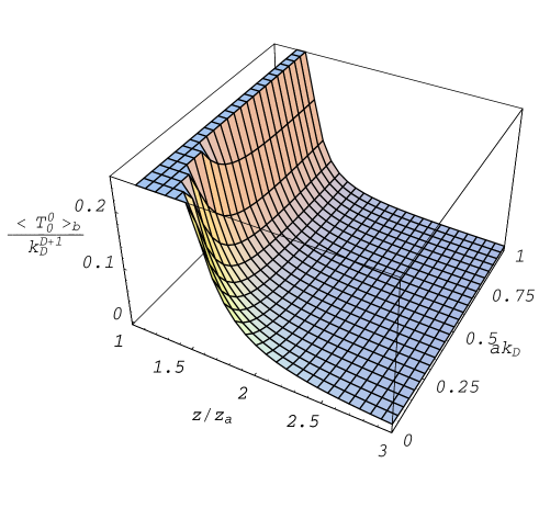
Figure 1: The part in the VEV of the energy density, $k_{D}^{-D-1}\langle T_{0}^{0}\rangle_{\mathrm{b}}$, induced by the brane as a function on $z/z_{a}$ and $ak_{D}$ for a minimally coupled massless scalar field in $D=4$.

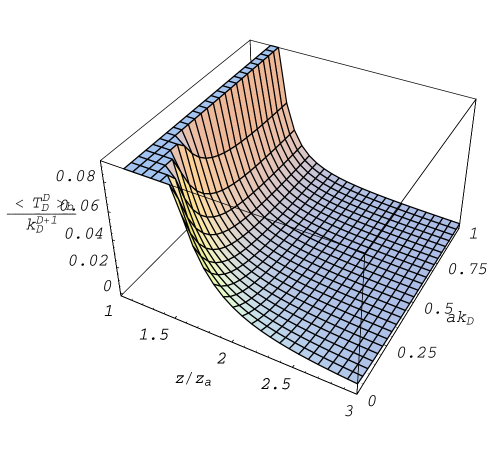
Figure 2: The part in the VEV of the radial stress, $k_{D}^{-D-1}\langle T_{D}^{D}\rangle_{\mathrm{b}}$, induced by the brane as a function on $z/z_{a}$ and $ak_{D}$ for a minimally coupled massless scalar field in $D=4$.

5.2 Interior region

Now let us consider the vacuum polarization effects inside the brane for the model with flat interior. The corresponding eigenfunctions have the form given by Eq. (2.8) with $f_{\lambda}(y)=R(y,k,\lambda)$ and the function $R(y,k,\lambda)$ is defined by formula (5.4). Substituting the eigenfunctions into the mode sum formula for the corresponding Wightman function one finds

$$\langle 0|\varphi(x)\varphi(x^{\prime})|0\rangle = \frac{z_{a}^{D}k_{D}^{D-1}}{\pi^{2}}\int d\mathbf{k\,}\frac{e^{i\mathbf{k}\cdot(\mathbf{x}-\mathbf{x}^{\prime})}}{(2\pi)^{D-1}}$$ (5.17)

$$\times\int_{0}^{\infty}d\lambda\,\frac{\lambda\cos(k_{y}y)\cos(k_{y}y^{\prime})e^{-i\sqrt{k^{2}+\lambda^{2}}(t-t^{\prime})}}{\cos^{2}(k_{y}a)\sqrt{k^{2}+\lambda^{2}}\left[\bar{J}_{\nu}^{2}(\lambda z_{a})+\bar{Y}_{\nu}^{2}(\lambda z_{a})\right]}.$$

For the evaluation of the expression on the right we use the relation

$$\frac{\cos^{-2}(k_{y}a)}{\bar{J}_{\nu}^{2}(\lambda z_{a})+\bar{Y}_{\nu}^{2}(\lambda z_{a})}=\frac{\pi k_{D}}{2k_{y}}\left[1-\frac{1}{2}\sum_{s=1,2}\frac{C\{e^{i\delta_{s}k_{y}a},H_{\nu}^{(s)}(\lambda z_{a})\}}{C\{\cos(k_{y}a),H_{\nu}^{(s)}(\lambda z_{a})\}}\right].$$ (5.18)

where $\delta_{s}=(-1)^{s+1}$, and for given functions $f(z)$ and $g(z)$ we have introduced the notation

$$C\left\{f(u),g(v)\right\}=vf(u)g^{\prime}(v)+\left[\left(\frac{D}{2}-2\xi D\right)f(u)-\frac{u}{ak_{D}}f^{\prime}(u)\right]g(v),$$ (5.19)

with $u=k_{y}a$ and $v=\lambda z_{a}$.

By taking into account identity (5.18), the Wightman function is written in the form

$$\langle 0|\varphi(x)\varphi(x^{\prime})|0\rangle = (z_{a}k_{D})^{D}\int d\mathbf{k\,}\frac{e^{i\mathbf{k}\cdot(\mathbf{x}-\mathbf{x}^{\prime})}}{(2\pi)^{D}}\int_{0}^{\infty}d\lambda\,\frac{\lambda e^{-i\sqrt{k^{2}+\lambda^{2}}(t-t^{\prime})}}{k_{y}\sqrt{k^{2}+\lambda^{2}}}$$ (5.20)

$$\times\cos(k_{y}y)\cos(k_{y}y^{\prime})\left[1-\frac{1}{2}\sum_{s=1,2}\frac{C\{e^{i\delta_{s}k_{y}a},H_{\nu}^{(s)}(\lambda z_{a})\}}{C\{\cos(k_{y}a),H_{\nu}^{(s)}(\lambda z_{a})\}}\right].$$

To transform the $\lambda$-integral with the first term in the square brackets, we present this integral as a sum of the integrals over the intervals $(0,me^{-k_{D}a})$ and $(me^{-k_{D}a},\infty)$. In the second integral changing the integration variable to $k_{y}$ we find

$$\int_{0}^{\infty}d\lambda\,\frac{\lambda e^{-i\sqrt{k^{2}+\lambda^{2}}(t-t^{\prime})}}{k_{y}\sqrt{k^{2}+\lambda^{2}}}\cos(k_{y}y)\cos(k_{y}y^{\prime})=e^{-2k_{D}a}\int_{0}^{\infty}dk_{y}\,\frac{e^{-i\sqrt{k^{2}+\lambda^{2}}(t-t^{\prime})}}{\sqrt{k^{2}+\lambda^{2}}}$$

$$\quad\times\cos(k_{y}y)\cos(k_{y}y^{\prime})-i\int_{0}^{me^{-k_{D}a}}d\lambda\,\frac{\lambda e^{-i\sqrt{k^{2}+\lambda^{2}}(t-t^{\prime})}}{\eta(\lambda)\sqrt{k^{2}+\lambda^{2}}}\cosh(y\eta(\lambda))\cosh(y^{\prime}\eta(\lambda)),$$ (5.21)

with the notation $\eta(\lambda)=\sqrt{m^{2}-\lambda^{2}e^{2k_{D}a}}$. In the first integral on the right of (5.21), $\lambda$ is a function of $k_{y}$ given by formula (5.4). Let us consider the $\lambda$-integral with the second term in the square brackets of (5.20). Note that in accordance with formula (5.4) for $k_{y}$, the corresponding integrand has branch point at $\lambda=me^{-k_{D}a}$. For definiteness we will assume that this point is circled from above by a semicircle of small radius in the complex $\lambda$-plane. With this choice, assuming that $|y|+|y^{\prime}|+|t-t^{\prime}|<2a$, we rotate the integration contour in the complex plane $\lambda$ by the angle $\pi/2$ for $s=1$ and by the angle $-\pi/2$ for $s=2$. In the second case the integral with $s=2$ is equal to the corresponding integral over the negative part of the imaginary axis plus the integral over the contour $C$ depicted in figure 3. By taking into account that on the upper/lower parts of the contour $C$ we have $k_{y}=\pm i\eta(\lambda)$, for this contribution one finds

$$-\int_{C}d\lambda\,\frac{\lambda\cos(k_{y}y)\cos(k_{y}y^{\prime})e^{-i\sqrt{k^{2}+\lambda^{2}}(t-t^{\prime})}}{2k_{y}\sqrt{k^{2}+\lambda^{2}}}\frac{C\{e^{-ik_{y}a},H_{\nu}^{(2)}(\lambda z_{a})\}}{C\{\cos(k_{y}a),H_{\nu}^{(2)}(\lambda z_{a})\}}$$

$$\quad=i\int_{0}^{me^{-k_{D}a}}d\lambda\,\frac{\lambda e^{-i\sqrt{k^{2}+\lambda^{2}}(t-t^{\prime})}}{\eta(\lambda)\sqrt{k^{2}+\lambda^{2}}}\cosh(y\eta(\lambda))\cosh(y^{\prime}\eta(\lambda)).$$ (5.22)

Now we see that the the integral over the contour $C$ cancels the second term on the right of (5.21). In the integrals over the imaginary axis the parts over the intervals $(0,ik)$ and $(0,-ik)$ cancel out. After introducing the modified Bessel functions, one can see that the Wightman function is presented in the form

$$\langle 0|\varphi(x)\varphi(x^{\prime})|0\rangle=G_{0}(x,x^{\prime})+G_{1}(x,x^{\prime}),$$ (5.23)

where

$$G_{0}(x,x^{\prime})=(z_{a}k_{D})^{D-2}\int\frac{d\mathbf{k}}{(2\pi)^{D}}e^{i\mathbf{k}\cdot(\mathbf{x}-\mathbf{x}^{\prime})}\int_{0}^{\infty}dk_{y}\,\frac{e^{-i\sqrt{k^{2}+\lambda^{2}}(t-t^{\prime})}}{\sqrt{k^{2}+\lambda^{2}}}\cos(k_{y}y)\cos(k_{y}y^{\prime}),$$ (5.24)

and

$$G_{1}(x,x^{\prime}) = -\frac{(z_{a}k_{D})^{D}}{(2\pi)^{D}}\int d\mathbf{k\,}e^{i\mathbf{k}\cdot(\mathbf{x}-\mathbf{x}^{\prime})}\int_{k}^{\infty}dx\,\frac{xC\{e^{-\varkappa(x)a},K_{\nu}(xz_{a})\}}{C\{\cosh(\varkappa(x)a),K_{\nu}(xz_{a})\}}$$ (5.25)

$$\times\frac{\cosh(\varkappa(x)y)\cosh(\varkappa(x)y^{\prime})}{\varkappa(x)\sqrt{x^{2}-k^{2}}}\cosh[\sqrt{x^{2}-k^{2}}(t-t^{\prime})].$$

In (5.25), $\varkappa(x)=\sqrt{x^{2}e^{2k_{D}a}+m^{2}}$, and we have used the notation (5.19) with $g(v)=K_{\nu}(v)$ and $f(u)=e^{-u},\cosh u$ for the numerator and denominator, respectively.

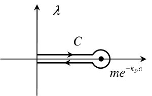
Figure 3: Integration contour $C$ in the complex $\lambda$-plane.

In (5.24) introducing a new integration variable $\mathbf{K}=\mathbf{k}e^{k_{D}a}$ we see that $G_{0}(x,x^{\prime})$ is the Wightman function in the Minkowski spacetime in coordinates (5.1) orbifolded along the $y$-direction:

$$G_{0}(x,x^{\prime})=\int d\mathbf{K\,}\frac{e^{i\mathbf{K}\cdot(\mathbf{X}-\mathbf{X}^{\prime})}}{(2\pi)^{D}}\int_{0}^{\infty}dk_{y}\,\frac{e^{-i\sqrt{K^{2}+k_{y}^{2}+m^{2}}(X^{0}-X^{0\prime})}}{\sqrt{K^{2}+k_{y}^{2}+m^{2}}}\cos(k_{y}y)\cos(k_{y}y^{\prime}),$$ (5.26)

where $\mathbf{X}=(X^{1},X^{2},\ldots,X^{D-1})$ with coordinates $X^{\mu}$ defined by relation (5.2). This function differs by the factor 1/2 from the Wightman function for a plate in the Minkowski spacetime located at $y=0$ on which the field obeys the Neumann boundary condition. Evaluating the integrals, function (5.26) is presented in the form

$$G_{0}(x,x^{\prime}) = \frac{1}{2}G_{M}(x,x^{\prime})+\frac{m^{(D-1)/2}}{2(2\pi)^{(D+1)/2}}$$ (5.27)

$$\times\frac{K_{(D-1)/2}\left(m\sqrt{|\mathbf{X}-\mathbf{X}^{\prime}|^{2}+(y+y^{\prime})^{2}-(X^{0}-X^{0\prime})^{2}}\right)}{\left(|\mathbf{X}-\mathbf{X}^{\prime}|^{2}+(y+y^{\prime})^{2}-(X^{0}-X^{0\prime})^{2}\right)^{(D-1)/4}},$$

where $G_{M}(x,x^{\prime})$ is the Wightman function for the Minkowski spacetime. Note that the expression for $G_{M}(x,x^{\prime})/2$ is given by the same formula as the second term on the right of (5.27) with the replacement $y+y^{\prime}\rightarrow y-y^{\prime}$. The term $G_{1}(x,x^{\prime})$ on the right of formula (5.23) is induced by the AdS geometry in the region $y>a$. For a conformally coupled massless scalar field one has $\nu=1/2$ and by using definition (5.19) it can be explicitly checked that $C\{e^{-u},K_{\nu}(u/ak_{D})\}=0$. Hence, in this case the part $G_{1}(x,x^{\prime})$ of the Wightman function vanishes.

Now we turn to the evaluation of the renormalized VEV for the field square. The renormalization corresponds to the omission of the part coming from the Minkowskian Wightman function in (5.27). As a result the VEV for the field square is presented in the form

$$\langle\varphi^{2}\rangle_{\mathrm{ren}}^{\mathrm{(int)}}=\langle\varphi^{2}\rangle_{0,\mathrm{ren}}^{\mathrm{(int)}}+\langle\varphi^{2}\rangle_{\mathrm{b}}^{\mathrm{(int)}}.$$ (5.28)

Here the part $\langle\varphi^{2}\rangle_{0,\mathrm{ren}}^{\mathrm{(int)}}$ is obtained from the second term on the right of (5.27) in the coincidence limit and is given by the formula

$$\langle\varphi^{2}\rangle_{0,\mathrm{ren}}^{\mathrm{(int)}}=\frac{m^{D-1}}{2(2\pi)^{(D+1)/2}}\frac{K_{(D-1)/2}\left(2my\right)}{\left(2my\right)^{(D-1)/2}}.$$ (5.29)

The second term in the right hand-side of formula (5.28) is obtained from (5.25) taking the coincidence limit of the arguments and using the formula

$$\int d\mathbf{k\,}\int_{k}^{\infty}dx\frac{k^{s}g(x)}{\sqrt{x^{2}-k^{2}}}=\frac{\pi^{(D-1)/2}}{\Gamma((D-1)/2)}B\left(\frac{D-1+s}{2},\frac{1}{2}\right)\int_{0}^{\infty}dx\,x^{D+s-2}g(x),$$ (5.30)

with $B(x,y)$ being the Euler beta function. This gives the result

$$\langle\varphi^{2}\rangle_{\mathrm{b}}^{\mathrm{(int)}}=-\frac{(4\pi)^{-D/2}}{\Gamma(D/2)}\int_{m}^{\infty}dx\,(x^{2}-m^{2})^{D/2-1}\cosh^{2}(xy)U_{\nu}(x),$$ (5.31)

with the notation

$$U_{\nu}(x)=\frac{C\{e^{-ax},K_{\nu}(\sqrt{x^{2}-m^{2}}/k_{D})\}}{C\{\cosh(ax),K_{\nu}(\sqrt{x^{2}-m^{2}}/k_{D})\}}.$$ (5.32)

This part in the VEV of the field square is induced by the AdS geometry in the exterior region. Note that if condition (5.8) is satisfied the denominator in (5.32) is negative. Recall that under this condition there are no modes with imaginary $\lambda$.

The integral on the right of formula (5.31) is finite for $|y|<a$ and diverges on the boundary of the brane $|y|=a$. In order to find the corresponding asymptotic behavior, we note that for points near the boundary the main contribution comes from large values $x$. By using the corresponding asymptotic formula for the function $K_{\nu}(x)$, to the leading order near the boundary $y=a$ we find

$$\langle\varphi^{2}\rangle_{\mathrm{b}}^{\mathrm{(int)}}\sim-\frac{k_{D}(\xi-\xi_{D})}{(4\pi)^{(D+1)/2}}\frac{D\Gamma((D-1)/2)}{(D-2)(a-y)^{D-2}}.$$ (5.33)

In the limit $am\gg 1$ the main contribution into the integral in formula (5.31) comes from the lower limit and one finds

$$\langle\varphi^{2}\rangle_{\mathrm{b}}^{\mathrm{(int)}}\approx-\frac{Bm^{D-1}\cosh^{2}(my)}{(4\pi am)^{D/2}}e^{-2am},\;B\equiv\frac{D/2-2\xi D+m/k_{D}-\nu}{D/2-2\xi D-m/k_{D}-\nu}.$$ (5.34)

As we could expect, in this limit the VEVs are exponentially suppressed. For large values of the AdS curvature assuming that $a,m\gg 1/k_{D}$, from definition (5.19) it is easily seen that under the conditions $\xi\gg 1/(ak_{D})$, $\xi-\xi_{D}\gg 1/(ak_{D})$ the asymptotic behavior of $\langle\varphi^{2}\rangle_{\mathrm{b}}^{\mathrm{(int)}}$ is obtained substituting in formula (5.31)

$$U_{\nu}(x)\approx\frac{2}{e^{2ax}+1}.$$ (5.35)

The corresponding expression coincides with the VEV induced by Dirichlet boundary located at $y=a$ in the Minkowski spacetime orbifolded along the $y$-direction with the fixed point $y=0$. For special cases of minimally and conformally coupled scalar fields, in the limit under consideration the leading terms are obtained substituting in (5.31)

$$U_{\nu}(x) \approx -\frac{2}{e^{2ax}-1},\;\xi=0,$$ (5.36)

$$U_{\nu}(x) \approx -\frac{2}{\frac{x+\sqrt{x^{2}-m^{2}}}{x-\sqrt{x^{2}-m^{2}}}e^{2ax}-1},\;\xi=\xi_{D}.$$ (5.37)

In the minimally coupled case the corresponding limiting value coincides with the VEV induced by Neumann boundary located at $y=a$ in the Minkowski spacetime orbifolded along the $y$-direction with the fixed point $y=0$.

Now let us consider the VEV for the energy-momentum tensor. As in the case of the field square, it is presented in the form

$$\langle T_{i}^{k}\rangle_{\mathrm{ren}}^{\mathrm{(int)}}=\langle T_{i}^{k}\rangle_{0,\mathrm{ren}}^{\mathrm{(int)}}+\langle T_{i}^{k}\rangle_{\mathrm{b}}^{\mathrm{(int)}},$$ (5.38)

where $\langle T_{ik}\rangle_{0,\mathrm{ren}}^{\mathrm{(int)}}$ is the vacuum energy-momentum tensor in the Minkowski spacetime in coordinates (5.1) orbifolded along the $y$-direction and the presence of the part $\langle T_{ik}\rangle_{\mathrm{b}}^{\mathrm{(int)}}$ is related to that the geometry in the region $y>a$ is AdS. For the first part one has (no summation over $i$)

$$\langle T_{i}^{i}\rangle_{0,\mathrm{ren}}^{\mathrm{(int)}}=\frac{m^{D+1}}{(4\pi my)^{(D+1)/2}}\left\{K_{(D+1)/2}\left(2my\right)\left(2\xi-1\right)+\left(1-4\xi\right)myK_{(D+3)/2}\left(2my\right)\right\},$$ (5.39)

with $\;i=0,1,\ldots,D-1$ and $\langle T_{D}^{D}\rangle_{0,\mathrm{ren}}^{\mathrm{(int)}}=0$. For a massless scalar field this leads to the result (no summation over $i$)

$$\langle T_{i}^{i}\rangle_{0,\mathrm{ren}}^{\mathrm{(int)}}=-\frac{D\left(\xi-\xi_{D}\right)}{(4\pi)^{(D+1)/2}y^{D+1}}\Gamma\left(\frac{D+1}{2}\right).$$ (5.40)

For the second term on the right of (5.38) we find (no summation over $i$)

$$\langle T_{i}^{i}\rangle_{\mathrm{b}}^{\mathrm{(int)}} = \frac{(4\pi)^{-D/2}}{\Gamma(D/2)}\int_{m}^{\infty}dx(x^{2}-m^{2})^{D/2}U_{\nu}(x)$$ (5.41)

$$\times\left\{\frac{1}{D}\cosh^{2}(xy)+\frac{\left(4\xi-1\right)x^{2}}{x^{2}-m^{2}}\left[\cosh^{2}(xy)-\frac{1}{2}\right]\right\},$$

$$\langle T_{D}^{D}\rangle_{\mathrm{b}}^{\mathrm{(int)}} = -\frac{(4\pi)^{-D/2}}{2\Gamma(D/2)}\int_{m}^{\infty}dx\,(x^{2}-m^{2})^{D/2-1}x^{2}U_{\nu}(x),$$ (5.42)

with $i=0,1,\ldots,D-1$, and the function $U_{\nu}(x)$ is defined by formula (5.32). Note that the radial stress inside the brane does not depend on spacetime point. This result could be also obtained directly from the continuity equation. As it has been mentioned before, for a conformally coupled massless scalar we have $U_{\nu}(x)=0$ and, hence, the parts in the VEV of the energy-momentum tensor given by formulae (5.41),(5.42) vanish. From formula (5.40) it follows that in this case the part $\langle T_{i}^{i}\rangle_{0,\mathrm{ren}}^{\mathrm{(int)}}$ vanishes as well.

Now let us consider the VEV of the energy-momentum tensor near the brane core. In the way similar to that for the exterior region we find (no summation over $i$)

$$\langle T_{i}^{i}\rangle_{\mathrm{b}}^{\mathrm{(int)}}\sim\frac{D-1}{Dk_{D}(y-a)}\langle T_{D}^{D}\rangle_{\mathrm{b}}^{\mathrm{(int)}}\sim\frac{Dk_{D}(\xi-\xi_{D})^{2}}{2^{D}\pi^{(D+1)/2}}\frac{\Gamma((D+1)/2)}{(a-y)^{D}},$$ (5.43)

with $i=0,1,\ldots,D-1$. For a conformally coupled scalar field the corresponding asymptotic behavior is given by formulae (5.14). In the limit $am\gg 1$ to the leading order one has (no summation over $i$)

$$\langle T_{i}^{i}\rangle_{\mathrm{b}}^{\mathrm{(int)}} \approx \frac{Bm^{D+1}e^{-2am}}{2(4\pi am)^{D/2}}(4\xi-1)\left[2\cosh^{2}(my)-1\right],$$ (5.44)

$$\langle T_{D}^{D}\rangle_{\mathrm{b}}^{\mathrm{(int)}} \approx -\frac{Bm^{D+1}e^{-2am}}{2(4\pi am)^{D/2}}.$$ (5.45)

For large values of the AdS curvature, $a,m\gg 1/k_{D}$, the leading terms for the VEV of the energy-momentum tensor are obtained from formulae (5.41),(5.42), by making substitutions (5.35) for $\xi\gg 1/(ak_{D})$, $\xi-\xi_{D}\gg 1/(ak_{D})$, and (5.36),(5.37) for minimally and conformally coupled scalars.

In figure 4 we have plotted the dependence of the part in the VEV of the energy density induced by the exterior AdS geometry in the region inside the brane as a function of $y/a$ and $ak_{D}$ for a minimally coupled massless scalar field in the case $D=4$.

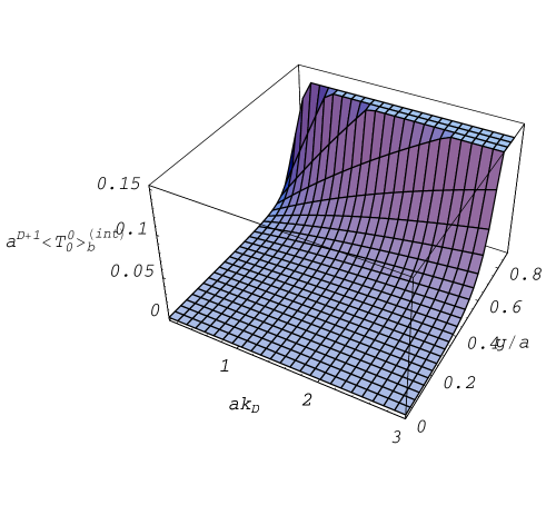
Figure 4: The energy density inside the brane, $a^{D+1}\langle T_{0}^{0}\rangle_{\mathrm{b}}^{\mathrm{(int)}}$, induced by the AdS geometry in the exterior region as a function on $ak_{D}$ and $y/a$ for a minimally coupled massless scalar field in $D=4$.

The corresponding radial stress does not depend on $y$ and is depicted in figures 5, 6 as a function of the parameters $am$ and $ak_{D}$ for minimally and conformally coupled fields, respectively. We recall that for a conformally coupled massless scalar field the corresponding VEVs vanish for both field square and the energy-momentum tensor. The perpendicular interior vacuum force acting per unit surface of the brane boundary is determined by $-\langle T_{D}^{D}\rangle_{\mathrm{b}}^{\mathrm{(int)}}$. As it is seen from figures 5, 6 for minimally and conformally coupled scalars these forces tend to decrease the brane thickness.

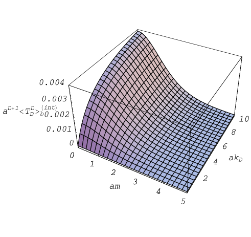
Figure 5: The part in the radial stress inside the brane, $a^{D+1}\langle T_{D}^{D}\rangle_{\mathrm{b}}^{\mathrm{(int)}}$, induced by the AdS geometry of the exterior region as a function on $am$ and $ak_{D}$ for a minimally coupled scalar field in $D=4$.

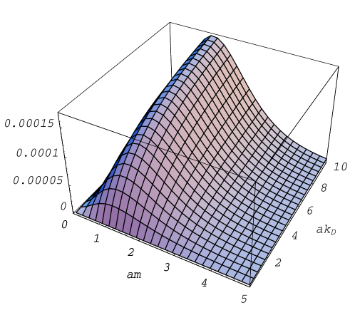
Figure 6: The same as in figure 5 for a conformally coupled scalar field.

6 Conclusion

In braneworld models the investigation of quantum effects is of considerable phenomenological interest, both in particle physics and in cosmology. In the present paper we have considered the one-loop vacuum effects for a massive scalar field with general curvature coupling parameter induced by a $Z_{2}$-symmetric thick brane on the $(D+1)$-dimensional AdS bulk. The previous papers on the investigation of the vacuum polarization by the gravitational field of the brane are mainly concerned with the idealized thin brane model, where the curvature has singularity at the location of the brane. Here we consider the general plane symmetric static model of the brane with finite thickness, described by the line element (2.2). Among the most important characteristics of the vacuum, which carry information about the internal structure of the brane, are the VEVs for the field square and the energy-momentum tensor. In order to obtain these expectation values we first construct the positive frequency Wightman function. In the region outside the brane this function is presented as a sum of two distinct contributions. The first one corresponds to the Wightman function in the free AdS geometry and the second one is induced by the brane. The latter is given by formula (2.30), where the tilted notation is defined by formula (2.31) with the coefficient from (2.32) for the model without an infinitely thin shell on the brane boundary. This coefficient is determined by the radial part of the interior eigenfunctions and describes the influence of the core properties on the vacuum characteristics in the exterior region. In the case of the model with a thin shell on the boundary of the brane, the derivatives of the metric tensor components are discontinuous on the brane surface. This leads to the delta function type contribution in the Ricci scalar and, hence in the equation for the radial eigenfunctions in the case of the non-minimally coupled scalar field. As a result, the radial eigenfunctions have a discontinuity in their slope at the brane boundary. This leads to an additional term in the coefficient of the tilted notation which is proportional to the trace of the surface energy-momentum tensor (see Eq. (3.10)).

By using the formula for the Wightman function, in section 4 we have investigated the influence of the non-trivial internal structure of the brane on the VEVs of the field square and the energy-momentum tensor. The parts in these VEVs induced by the brane are directly obtained from the corresponding part of the Wightman function for the case of the field square and by applying on this function a certain second-order differential operator and taking the coincidence limit for the energy-momentum tensor. In the general plane symmetric model for the brane interior these parts are given by formulae (4.2) and (4.10) for the field square and the energy-momentum tensor respectively. These formulae are further simplified for models with Poincare invariance along the directions parallel to the brane taking the form (4.5), (4.14). For a conformally coupled massless scalar field the corresponding energy-momentum tensor vanishes. The parts in the VEVs of the field square and energy-momentum tensor induced by the brane diverge on the boundary of the brane. The surface divergences in the VEVs of the local observables are well–known in quantum field theory with boundaries and are investigated for various boundary geometries. At large distances from the brane the brane induced VEVs are suppressed by the factor $e^{-2\nu k_{D}y}$. In the limit of strong gravitational fields corresponding to large values of the AdS energy scale $k_{D}$, for points not too close to the brane the parts in the VEVs induced by the brane behave as $k_{D}^{D\pm 1}e^{-2\nu k_{D}(y-a)}$ with upper/lower sign corresponding to the energy-momentum tensor/field square. In this case the relative contribution of the brane induced effects are exponentially suppressed with respect to the free AdS part.

As an application of the general results, in section 5 we have considered a simple model with flat spacetime in the region inside the brane. The corresponding surface energy-momentum tensor on the boundary of the brane is obtained from the matching conditions and has the form given by Eq. (5.3). The brane induced parts of the exterior VEVs in this model are obtained from the general results by taking the function in the coefficient of the tilted notation from Eq. (5.7). We have also investigated the vacuum densities inside the brane. Though the spacetime geometry inside the brane is Monkowskian, the AdS geometry of the exterior region induces vacuum polarization effects in this region as well. In order to find the corresponding renormalized VEVs of the field square and the energy-momentum tensor we have presented the Wightman function in the interior region in decomposed form (5.23). In this representation the first term on the right is the Wightman function in the Minkowski spacetime orbifolded along the direction perpendicular to the brane and the second one is induced by the AdS geometry in the exterior region. The corresponding parts in the VEVs of the field square and the energy-momentum tensor are given by formulae (5.31), (5.41), (5.42) and are investigated in various asymptotic limits of the parameters. For a massless conformally coupled scalar field these parts vanish. In the general case of the curvature coupling parameter, the corresponding radial stress is uniform inside the brane and determine the interior vacuum forces acting on the boundary of the brane. The results of the numerical calculations plotted in figures 5, 6 show that for both minimally and conformally coupled scalar fields these forces tend to decrease the thickness of the brane. When the brane thickness tends to zero, from the formulae of the model with flat interior the corresponding results in the RS 1-brane model are obtained.

References

- [1] V.A. Rubakov, Phys. Usp. 44, 871 (2001); R. Maartens, Living Rev. Relativity 7, 7 (2004).
- [2] L. Randall and R. Sundrum, Phys. Rev. Lett. 83, 3370 (1998).
- [3] L. Randall and R. Sundrum, Phys. Rev. Lett. 83, 4690 (1998).
- [4] M. Fabinger and P. Horava, Nucl. Phys. B580, 243 (2000).
- [5] S. Nojiri, S.D. Odintsov, and S. Zerbini, Phys. Rev. D 62, 064006 (2000); S. Nojiri and S. Odintsov, Phys. Lett. B 484, 119 (2000).
- [6] D.J. Toms, Phys. Lett. B 484, 149 (2000).
- [7] S. Nojiri, O. Obregon, and S.D. Odintsov, Phys. Rev. D 62, 104003 (2000).
- [8] W. Goldberger and I. Rothstein, Phys. Lett. B 491, 339 (2000).
- [9] S. Nojiri, S.D. Odintsov, and S. Zerbini, Class. Quant. Grav. 17, 4855 (2000); S. Nojiri and S. Odintsov, J. High Energy Phys. 0007, 049 (2000).
- [10] J. Garriga, O. Pujolas, and T. Tanaka, Nucl. Phys. B605, 192 (2001).
- [11] S. Mukohyama, Phys. Rev. D 63, 044008 (2001).
- [12] R. Hofmann, P. Kanti, and M. Pospelov, Phys. Rev. D 63, 124020 (2001).
- [13] I. Brevik, K.A. Milton, S. Nojiri, and S.D. Odintsov, Nucl. Phys. B599, 305 (2001).
- [14] A. Flachi and D.J. Toms, Nucl. Phys. B610, 144 (2001).
- [15] P.B. Gilkey, K. Kirsten, and D.V. Vassilevich, Nucl. Phys. B601, 125 (2001).
- [16] A. Flachi, I.G. Moss, and D.J. Toms, Phys. Lett. B 518, 153 (2001); Phys. Rev. D 64, 105029 (2001).
- [17] W. Naylor and M. Sasaki, Phys. Lett. B 542, 289 (2002).
- [18] A.A. Saharian and M.R. Setare, Phys. Lett. B 552, 119 (2003).
- [19] E. Elizalde, S. Nojiri, S.D. Odintsov, and S. Ogushi, Phys. Rev. D 67, 063515 (2003).
- [20] J. Garriga and A. Pomarol, Phys. Lett. B 560, 91 (2003).
- [21] S. Nojiri and S.D. Odintsov, J. Cosmol. Astropart. Phys. 06, 004 (2003).
- [22] A.H. Yeranyan and A.A. Saharian, Astrophysics 46, 386 (2003).
- [23] I.G. Moss, W. Naylor, W. Santiago-Germán, and M. Sasaki, Phys. Rev. D 67 125010 (2003).
- [24] A.A. Saharian and M.R. Setare, Phys. Lett. B 584, 306 (2004).
- [25] G. Cognola, E. Elizalde, S. Nojiri, S. D. Odintsov, and S. Zerbini, Mod. Phys. Lett. A 19, 1435 (2004).
- [26] A. Knapman and D.J. Toms, Phys. Rev. D 69, 044023 (2004).
- [27] A.A. Saharian, Astrophysics 47, 303 (2004).
- [28] S. Nojiri and S.D. Odintsov, Phys. Rev. D 69, 023511 (2004).
- [29] A.A. Saharian and M.R. Setare, Phys. Lett. B 584, 306 (2004).
- [30] J.P. Norman, Phys.Rev. D 69, 125015 (2004).
- [31] A.A. Saharian, Phys. Rev. D 70, 064026 (2004); A.A. Saharian, Astrophysics 48, 122 (2005).
- [32] O. Pujolàs and T. Tanaka, J. Cosmol. Astropart. Phys. 12, 009 (2004).
- [33] M.R. Setare, Eur. Phys. J. C 38, 373 (2004).
- [34] A.A. Saharian, Nucl. Phys. B712, 196 (2005).
- [35] W. Naylor and M. Sasaki, Prog. Theor. Phys. 113, 535 (2005).
- [36] A.A. Saharian and M.R. Setare, Nucl. Phys. B724, 406 (2005); A. A. Saharian and M. R. Setare, J. High Energy Phys. 02, 089 (2007).
- [37] O. Pujolàs and M. Sasaki, J. Cosmol. Astropart. Phys. 09, 002 (2005).
- [38] M.R. Setare, Phys. Lett. B 620, 111 (2005).
- [39] E. Elizalde, J. Phys. A 39, 6299 (2006).
- [40] M. Minamitsuji, W. Naylor, and M. Sasaki, Nucl. Phys. B737, 121 (2006); M. Minamitsuji, W. Naylor, and M. Sasaki, Phys. Lett. B 633, 607 (2006).
- [41] M.R. Setare, Phys. Lett. B 637, 1 (2006).
- [42] A.A. Saharian and M.R. Setare, Phys. Lett. B 637, 5 (2006).
- [43] A. Flachi, J. Garriga, O. Pujolàs, and T. Tanaka, J. High Energy Phys. 0308, 053 (2003); A. Flachi and O. Pujolàs, Phys. Rev. D 68, 025023 (2003); A.A. Saharian, Phys. Rev. D 73, 044012 (2006); A.A. Saharian, Phys. Rev. D 73, 064019 (2006); A.A. Saharian, Phys. Rev. D 74, 124009 (2006).
- [44] O. DeWolfe, D.Z. Freedman, S.S. Gubser, and A. Karch, Phys. Rev. D 62, 046008 (2000); M. Gremm, Phys. Lett. B 478, 434 (2000); C. Csaki, J. Erlich, T.J. Hollowood, and Y. Shirman, Nucl. Phys. B581, 309 (2000); S. Kobayashi, K. Koyama, and J. Soda, Phys. Rev. D 65, 064014 (2002); P. Mounaix and D. Langlois, Phys. Rev. D 65, 103523 (2002); N. Sasakura, J. High Energy Phys. 0202, 026 (2002); N. Sasakura, Phys. Rev. D 66, 065006 (2002); R. Mansouri, M. Borhani, and S. Khakshournia, Int. J. Mod. Phys. A 19, 4687 (2004); K.A. Bronnikov and B.E. Meierovich, Grav. Cosmol. 9, 313 (2003); O. Castillo-Felisola, A. Melfo, N. Pantoja, and A. Ramírez, Phys.Rev. D 70, 104029 (2004); I. Navarro and J. Santiago, JCAP 0603, 015 (2006); N. Barbosa-Candejas and A. Herrera-Aguilar, J. High Energy Phys. 0510, 101 (2005); V. Dzhunushaliev, gr-qc/0603020; S. Ghassemi, S. Khakshournia, and R. Mansouri, J. High Energy Phys. 0608, 019 (2006); N. Barbosa-Candejas and A. Herrera-Aguilar, Phys.Rev. D 73, 084022 (2006); R. Moderski and M. Rogatko, Phys. Rev. D 74, 044002 (2006); S. Ghassemi, S. Khakshournia, and R. Mansouri, gr-qc/0609132.
- [45] N.D. Birrell and P.C.W. Davis, Quantum Fields in Curved Space (Cambridge University Press, 1982).
- [46] P. Breitenlohner and D.Z. Freedman, Phys. Lett. B 115, (1982); P. Breitenlohner and D.Z. Freedman, Ann. Phys. (N.Y.) 144, 249 (1982); L. Mezincescu and P.K. Townsend, Ann.Phys. (N.Y.) 160, 406 (1985).
- [47] C.P. Burgess and C.A. Lütken, Phys. Lett. B 153, 137 (1985); R. Camporesi, Phys. Rev. D 43, 3958 (1991); M. Camela and C.P. Burgess, Can. J. Phys. 77, 85 (1999); M.M. Caldarelli, Nucl. Phys. B549, 499 (1999).
- [48] A.A. Saharian, Phys. Rev. D 69, 085005 (2004).
- [49] A.P. Prudnikov, Yu.A. Brychkov, and O.I. Marichev, Integrals and series, vol.2 (Gordon & Breach, New York, 1986).
- [50] B. Allen and A.C. Ottewill, Phys. Rev. D 42, 2669 (1990); B. Allen, B.S. Kay, and A.C. Ottewill, Phys. Rev. D 53, 6829 (1996); E.R. Bezerra de Mello, V.B. Bezerra, A.A. Saharian, and A.S. Tarloyan, Phys. Rev. D 74, 025017 (2006); E. R. Bezerra de Mello and A. A. Saharian, J. High Energy Phys. 0610, 049 (2006); E. R. Bezerra de Mello and A. A. Saharian, Phys. Rev. D 75, 065019 (2007).
- [51] Handbook of Mathematical Functions, edited by M. Abramowitz and I.A. Stegun (Dover, New York, 1972).