The meeting problem in the quantum random walk

Abstract

We study the motion of two non-interacting quantum particles performing a random walk on a line and analyze the probability that the two particles are detected at a particular position after a certain number of steps (meeting problem). The results are compared to the corresponding classical problem and differences are pointed out. Analytic formulas for the meeting probability and its asymptotic behavior are derived. The decay of the meeting probability for distinguishable particles is faster then in the classical case, but not quadratically faster. Entangled initial states and the bosonic or fermionic nature of the walkers are considered.

1 Introduction

Random walks are a long studied problem not only in classical physics but also in many other branches of science [1]. Random walks help to understand complex systems, their dynamics and the connection between dynamics and the underlying topological structure. More recently, quantum analogues [2, 3] of the classical random walks attracted considerable attention.

Quantum walks have been introduced in the early nineties by Aharonov, Davidovich and Zagury [2]. Since that the topic attracted considerable interest. The continuing attraction of the topic can be traced back to at least two reasons. First of all, the quantum walk is, as a topic, of sufficient interest on its own right because there are fundamental differences compared to the classical random walk. Next, quantum walks offer quite a number of possible applications. One of the best known is the link between quantum walks and quantum search algorithms which are superior to their classical counterparts [4, 5]. Another goal is to find new, efficient quantum algorithms by studying various types of quantum walks. Let us point out that from a quantum mechanical point of view there is no randomness involved in the time evolution of a quantum walk. The evolution of the walker is determined completely by a unitary time evolution. This applies to the two most common forms: the discrete [2] and the continuous time [5] quantum walks. For a review on quantum walks see for instance [3].

Several aspects of quantum walks have been analyzed. First of all quite much attention was paid to the explanation of the asymptotics of the unusual walker probability distribution using various approaches [6, 7, 8, 9]. Next, attention was paid to the explanation of the unusual probability distribution as a wave phenomenon [7, 13]. This question is of particular interest as there are several proposals how to realize quantum walks [10, 11, 12, 13, 14, 15, 16, 17], in particular proposals using optical elements as the basic blocks for the quantum walks [12, 13]. Among the first ones was the optical implementation of a Galton board [14]. An ion trap proposal as well as an neutral atom implementation was put forward few years later [15, 16, 17]. The neutral atom proposal lead to a real experiment in the year 2003 [18].

Apart from the studies of elementary random walks its generalizations have been studied [19]. Generalizations of random walks to higher dimensions [20] have been put forward and differences to the simpler models pointed out. Next the effect of randomness in optical implementations on quantum walks was analyzed and its link to localization pointed out [21]. Among further generalizations also the behavior of more than one walker (particle) in networks realizing random walks has been studied [22, 23]. The aim of the present paper is to add to this line of studies. We wish to study the evolution of two walkers performing a random walk. The evolution of each of the two walkers is subjected to the same rules. One of the interesting questions when two walkers are involved is to clarify how the probability of the walkers to meet changes with time (or number of steps taken in walk). Because the single quantum walker behavior differs from its classical counterpart it has to be expected that the same will apply to the situation when two walkers are involved. Interference, responsible for the unusual behavior of the single walker should play also a considerable role when two walkers will be involved. The possibility to change the input states (in particular the possibility to choose entangled initial walker states) adds another interesting point to the analysis. In the following, we will study the evolution of the meeting probability for two walkers. We point out the differences to the classical case and discuss the influence of the input state on this probability.

The paper is organized as follows - first we make a brief review of the concept of the discrete time quantum walk on an infinite line and its properties. Based on this we generalize the two particle random walk for both distinguishable and indistinguishable walkers and define the meeting problem. This problem is analyzed in section 3. The asymptotic behavior of the meeting probability is derived. Further the effect of entanglement and indistinguishability of the walkers is examined. In the conclusions we summarize the obtained results and discuss possible development. Finally, in the appendix the properties of the meeting problem in the classical random walk are derived.

2 Description of the walk

We first briefly summarize the description of the quantum random walk, for more details see e.g. [3]. We consider a coined random walk on an infinite line. The Hilbert space of the particle $\mathcal{H}$ consists of the position space $\mathcal{H}_{P}$ with the basis $\left\{|m\rangle|m\in\mathrm{Z}\right\}$, which is augmented by a coin space

$$\mathcal{H}_{C}=\left\{|L\rangle,|R\rangle\right\}.$$ (1)

The particle moves on the grid in discrete time steps in dependence on the coin state, the operator which induces a single displacement has the form

$$S=\sum_{m}|m-1\rangle\langle m|\otimes|L\rangle\langle L|+\sum_{m}|m+1\rangle\langle m|\otimes|R\rangle\langle R|.$$ (2)

A single step of the particle consists of a rotation of the coin state given by an arbitrary unitary matrix $C$ and the conditional displacement $S$. The time evolution operator $U$ describing one step of the random walk takes the form

$$U=S(I\otimes C).$$ (3)

If the initial state of the walker is $|\psi(0)\rangle$, then after $t$ steps its state will be given by the successive application of $U$ on the initial state

$$|\psi(t)\rangle=U^{t}|\psi(0)\rangle.$$ (4)

The probability distribution generated by such a random walk is given by

$$P(m,t)=|\langle m,L|\psi(t)\rangle|^{2}+|\langle m,R|\psi(t)\rangle|^{2}.$$ (5)

In our paper we concentrate on a particular case when the rotation of the coin is given by the Hadamard transformation

$$H=\frac{1}{\sqrt{2}}\left(\begin{array}[]{cc}1&1\\ 1&-1\\ \end{array}\right),$$ (6)

since this is the most studied example of an unbiased random walk. For quantum walks with arbitrary unitary coin see e.g. [24].

We will describe the wave-function of the walker at time $t$ by the set of two-component vectors of the form

$$\psi(m,t)=\left(\begin{array}[]{c}\psi_{L}(m,t)\\ \psi_{R}(m,t)\\ \end{array}\right),$$ (7)

where $\psi_{L}(m,t)$ ($\psi_{R}(m,t)$) is the probability amplitude that the walker is at time $t$ on the site $m$ with the coin state $|L\rangle$ ($|R\rangle$). The wave-function thus has the form

$$|\psi(t)\rangle=\sum_{m}\left(\psi_{L}(m,t)|m,L\rangle+\psi_{R}(m,t)|m,R\rangle\right).$$ (8)

Throughout the text we will use symbols $|\psi^{L(R)}(t)\rangle$, $\psi^{L(R)}_{i,j}(m,t)$ for the vectors and the probability amplitudes, under the assumption that the initial state of the walker was

$$|\psi^{L(R)}(0)\rangle=|0,L(R)\rangle,$$ (9)

similarly $P^{L(R)}(m,t)$ will be the corresponding probabilities.

From the time evolution of the wave-function (4) follows the dynamics of the two-component vectors $\psi(m,t)$

$$\psi(m,t+1)=\frac{1}{\sqrt{2}}\left(\begin{array}[]{cc}0&0\\ 1&-1\\ \end{array}\right)\psi(m-1,t)+\frac{1}{\sqrt{2}}\left(\begin{array}[]{cc}1&1\\ 0&0\\ \end{array}\right)\psi(m+1,t).$$ (10)

Thus the description of the time evolution of the walker reduces to a set of difference equations. Nayak and Vishwanath in [6] have found the analytical solution of (10) and derived the asymptotic form of the probability distribution. Before we proceed with the generalization of the quantum walk for two particles we will summarize the properties of the single walker probability distribution derived in [6], which we will use later for the estimation of the meeting probability. According to [6] the probability distribution of one walker is almost uniform in the interval $(s-t/\sqrt{2},s+t/\sqrt{2})$, where $s$ is the initial position of the walker, with the value $\approx 1/t$. Around the points $s\pm t/\sqrt{2}$ are peaks of width of the order of $t^{1/3}$ and the probability is approximately $t^{-2/3}$. Outside this region the probability decays faster then any inverse polynomial in $t$ and therefore we will neglect this part. We will also use the slow oscillating part of the walker probability distribution derived in [6] which has the form

$$P^{L(R)}_{slow}(x,t)=\frac{2}{\pi t\left(1\pm\frac{x}{t}\right)\sqrt{1-\frac{2x^{2}}{t^{2}}}},$$ (11)

for the case that the initial coin state was $L(R)$.

The main difference between classical and quantum random walk on a line is the shape of the probability distribution. Due to the interference effect the quantum walker spreads quadratically faster than the classical one and its variance goes like $\sigma\sim t$, in contrast with the result for the classical case $\sigma\sim\sqrt{t}$.

To visualize the properties of the quantum walk we plot in figure 1 the probability distribution and the slow-varying estimation. The initial conditions of the coin were chosen to be $\frac{1}{\sqrt{2}}(|L\rangle+i|R\rangle)$, which leads to an unbiased distribution. The slow-varying estimation for the symmetric probability distribution is given by

$$P^{sym}_{slow}(x,t)=\frac{1}{2}\left(P^{L}_{slow}(x,t)+P^{R}_{slow}(x,t)\right)=\frac{2}{\pi t\left(1-\frac{x^{2}}{t^{2}}\right)\sqrt{1-\frac{2x^{2}}{t^{2}}}}.$$ (12)

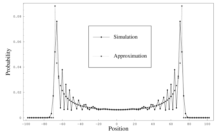
Figure 1: Probability distribution of a quantum random walker after 100 steps and the slow-varying estimation.

Using this description of the random walk we now proceed to the analysis of the random walk for two non-interacting distinguishable and indistinguishable particles.

2.1 Distinguishable walkers

The Hilbert space of the two walkers is given by a tensor product of the single walker spaces, i.e.

$$\mathcal{H}=(\mathcal{H}_{P}\otimes\mathcal{H}_{C})_{1}\otimes(\mathcal{H}_{P}\otimes\mathcal{H}_{C})_{2}.$$ (13)

Each walker has its own coin which determines his movement on the line. Since we assume that there is no interaction between the two walkers they evolve independently and the time evolution of the whole system is given by a tensor product of the single walker time evolution operators (3). We describe the state of the system by vectors

$$\psi(m,n,t)=\left(\begin{array}[]{c}\psi_{LL}(m,n,t)\\ \psi_{RL}(m,n,t)\\ \psi_{LR}(m,n,t)\\ \psi_{RR}(m,n,t)\\ \end{array}\right),$$ (14)

where e.g. the component $\psi_{RL}(m,n,t)$ is the amplitude of the state where the first walker is on $m$ with the internal state $|R\rangle$ and the second walker is on $n$ with the internal state $|L\rangle$. The state of the two walkers at time $t$ is then given by

$$|\psi(t)\rangle=\sum_{m,n}\sum_{i,j=\ R,L}\psi_{ij}(m,n,t)|m,i\rangle_{1}|n,j\rangle_{2}.$$ (15)

The conditional probability that the first walker is on a site $m$ at time $t$, provided that the second walker is at the same time at site $n$, is defined by

$$P(m,n,t)=\sum_{i,j=L,R}|\langle m,i|\langle n,j|\psi(t)\rangle|^{2}=\sum_{i,j=L,R}|\psi_{ij}(m,n,t)|^{2}.$$ (16)

Note that if we would consider a single random walker but on a two dimensional lattice, with two independent Hadamard coins for each spatial dimension, (16) will give the probability distribution generated by such a two dimensional walk. This shows the relation between a one dimensional walk with two walkers and a two dimensional walk.

The reduced probabilities for the first and the second walker are given by

$$P_{1}(m,t)=\sum_{n}P(m,n,t),\quad P_{2}(n,t)=\sum_{m}P(m,n,t).$$ (17)

We can rewrite them with the help of the reduced density operators of the corresponding walkers

$$\rho_{i}(t)=Tr_{j\neq i}|\psi(t)\rangle\langle\psi(t)|,$$ (18)

in the form

$$P_{i}(m,t)=\sum_{j}\langle m,j|\rho_{i}(t)|m,j\rangle.$$ (19)

The dynamics of the two walkers is determined by the single walker motion. Since we can always decompose the initial state of the two walkers into a linear combination of a tensor product of a single walker states and because the time evolution is also given by a tensor product of two unitary operators, the shape of the state will remain unchanged. Thus we can fully describe the time evolution of the two random walkers with the help of the single walker wave-functions. A similar relation holds for the probability distribution (16). Moreover, in the particular case when the two walkers are initially in a factorized state

$$|\psi(0)\rangle=\left(\sum_{m,i}\psi_{1i}(m,0)|m,i\rangle_{1}\right)\otimes\left(\sum_{n,j}\psi_{2j}(n,0)|n,j\rangle_{2}\right),$$ (20)

which translates into $\psi_{ij}(m,n,0)=\psi_{1i}(m,0)\psi_{2j}(n,0)$, the probability distribution remains a product of single walker probability distributions

$$P(m,n,t) = (|\psi_{1L}(m,t)|^{2}+|\psi_{1R}(m,t)|^{2})(|\psi_{2L}(n,t)|^{2}+|\psi_{2R}(n,t)|^{2})$$ (21)

$$= P_{1}(m,t)P_{2}(n,t).$$

However, when the initial state of the two walkers is entangled

$$|\psi(0)\rangle=\sum_{\alpha}\left\{\left(\sum_{m,i}\psi^{\alpha}_{1i}(m,0)|m,i\rangle_{1}\right)\otimes\left(\sum_{n,j}\psi^{\alpha}_{2j}(n,0)|n,j\rangle_{2}\right)\right\},$$ (22)

the probability distribution cannot be expressed in terms of single walker distributions but probability amplitudes

$$P(m,n,t)=\sum_{i,j=L,R}\left|\sum_{\alpha}\psi^{\alpha}_{1i}(m,t)\psi^{\alpha}_{2j}(n,t)\right|^{2}.$$ (23)

As we have shown above, when the two walkers are initially in a factorized state, the probability distribution (21) is a product of the reduced distributions and thus the positions of the walkers are independent. On the other hand, when they are entangled, the probability distribution differs from a product of the reduced probabilities and the positions of the walkers are correlated. However, notice that the correlations are present also in the classical random walk with two walkers, if we consider initial conditions of the following form

$$P(m,n,0)=\sum_{\alpha}P_{1}^{\alpha}(m,0)P_{2}^{\alpha}(n,0).$$ (24)

The difference between (23) and (24) is that in the quantum case we have probability amplitudes not probabilities. The effect of the quantum mechanical dynamics is the interference in (23).

Let us now define the meeting problem. We ask for the probability that the two walkers will be detected at the position $m$ after $t$ steps. This probability is given by the norm of the vector $\psi(m,m,t)$

$$M_{D}(m,t)=\sum_{i,j=L,R}|\psi_{ij}(m,m,t)|^{2}=P(m,m,t).$$ (25)

As we have seen above for a particular case when the two walkers are initially in a factorized state of the form (20) this can be further simplified to the multiple of the probabilities that the individual walkers will reach the site. However, this not possible in the situation when the walkers are initially entangled (22). The entanglement introduced in the initial state of the walkers leads to the correlations between the walkers position and thus the meeting probability is no longer a product of the single walker probabilities.

2.2 Indistinguishable walkers

We now analyze the situation when the two walkers are indistinguishable. Because we work with indistinguishable particles we use the Fock space and creation operators, we use symbols $a_{(m,i)}^{\dagger}$ for bosons and $b_{(n,j)}^{\dagger}$ for fermions, e.g. $a_{(m,i)}^{\dagger}$ creates one bosonic particle at position $m$ with the internal state $|i\rangle$. The time evolution is now given by the transformation of the creation operators, e.g. for bosons a single displacement is described by the following transformation of the creation operators

$$a_{(m,L)}^{\dagger} \longrightarrow \frac{1}{\sqrt{2}}\left(a_{(m-1,L)}^{\dagger}+a_{(m+1,R)}^{\dagger}\right)$$

$$a_{(m,R)}^{\dagger} \longrightarrow \frac{1}{\sqrt{2}}\left(a_{(m-1,L)}^{\dagger}-a_{(m+1,R)}^{\dagger}\right),$$ (26)

similarly for the fermionic walkers. The dynamics is defined on a one-particle level. We will describe the state of the system by the same vectors $\psi(m,n,t)$ as for the distinguishable walkers. The state of the two bosonic and fermionic walkers analogous to (15) for the distinguishable is given by

$$|\psi_{B}(t)\rangle = \sum_{m,n}\sum_{i,j=L,R}\frac{1}{2}(\psi_{ij}(m,n,t)+\psi_{ji}(n,m,t))a_{(m,i)}^{\dagger}a_{(n,j)}^{\dagger}|vac\rangle,$$

$$|\psi_{F}(t)\rangle = \sum_{m,n}\sum_{i,j=L,R}\frac{1}{2}(\psi_{ij}(m,n,t)-\psi_{ji}(n,m,t))b_{(m,i)}^{\dagger}b_{(n,j)}^{\dagger}|vac\rangle,$$ (27)

where $|vac\rangle$ is the vacuum state. In the case of two bosonic walkers initially in the same state we have to include an additional factor of $1/\sqrt{2}$, to ensure proper normalization.

The conditional probability distribution is given by

$$P_{B,F}(m,n,t) = \sum_{i,j=L,R}|\langle 1_{(m,i)}1_{(n,j)}|\psi_{B,F}(t)\rangle|^{2}$$ (28)

$$= \sum_{i,j=L,R}|\psi_{ij}(m,n,t)\pm\psi_{ji}(n,m,t)|^{2},$$

for $m\neq n$, and for $m=n$

$$P_{B}(m,m,t) = |\langle 2_{(m,L)}|\psi_{B}(t)\rangle|^{2}+|\langle 2_{(m,R)}|\psi_{B}(t)\rangle|^{2}+$$

$$\quad+|\langle 1_{(m,L)}1_{(m,R)}|\psi_{B}(t)\rangle|^{2}$$

$$= 2|\psi_{LL}(m,m,t)|^{2}+2|\psi_{RR}(m,m,t)|^{2}+$$

$$\quad+|\psi_{LR}(m,m,t)+\psi_{RL}(m,m,t)|^{2}$$

$$= M_{B}(m,t),$$

$$P_{F}(m,m,t) = |\langle 1_{(m,L)}1_{(m,R)}|\psi_{F}(t)\rangle|^{2}$$ (29)

$$= |\psi_{LR}(m,m,t)-\psi_{RL}(m,m,t)|^{2}$$

$$= M_{F}(m,t).$$

The diagonal terms of the probability distribution (2.2) define the meeting probability we wish to analyze.

Let us now specify the meeting probability for the case when the probability amplitudes can be written in a factorized form $\psi_{ij}(m,n,t)=\psi_{1i}(m,t)\psi_{2j}(n,t)$, which for the distinguishable walkers corresponds to the situation when they are initially not correlated. In this case the meeting probabilities are given by

$$M_{B}(m,t)=2|\psi_{1L}(m,t)\psi_{2L}(m,t)|^{2}+2|\psi_{1R}(m,t)\psi_{2R}(m,t)|^{2}$$

$$+|\psi_{1L}(m,t)\psi_{2R}(m,t)+\psi_{1R}(m,t)\psi_{2L}(m,t)|^{2},$$ (30)

for bosons and

$$M_{F}(m,t)=|\psi_{1L}(m,t)\psi_{2R}(m,t)-\psi_{1R}(m,t)\psi_{2L}(m,t)|^{2},$$ (31)

for fermions. We see that they differ from the formulas for the distinguishable walkers, except a particular case when the two bosons start in the same state, i. e. $\psi_{1}(m,0)=\psi_{2}(m,0)=\psi(m,0)$ for all integers $m$. For this initial state we get

$$M_{B}(m,t) = |\psi_{L}(m,t)|^{4}+|\psi_{R}(m,t)|^{4}+2|\psi_{L}(m,t)\psi_{R}(m,t)|^{2}$$ (32)

$$= (|\psi_{L}(m,t)|^{2}+|\psi_{R}(m,t)|^{2})^{2}$$

$$= P^{2}(m,t),$$

which is the same as for the case of distinguishable walkers starting at the same point with the same internal state.

We conclude this section by emphasizing that except the case of two bosons with the same initial state the probability of meeting differs from the case of distinguishable particles and we have to use the probability amplitudes, whereas for the distinguishable walkers we can reduce it to one-particle probabilities.

3 Analysis of the meeting problem

Let us now compare the meeting problem in the classical and quantum case. We will study the two following two probabilities: the total probability of meeting after $t$ step have been performed defined by

$$M(t)=\sum_{m}M(m,t),$$ (33)

and the overall probability of meeting during some period of steps $T$ defined as

$$\overline{M}(T)=1-\prod_{t=1}^{T}\left(1-M(t)\right).$$ (34)

The total probability of meeting $M(t)$ is the probability that the two walkers meet at time $t$ anywhere on the lattice, the overall probability of meeting $\overline{M}(T)$ is the probability that they meet at least once anywhere on the lattice during the first $T$ steps.

3.1 Distinguishable walkers

We first concentrate on the influence of the initial state on the meeting probability for the distinguishable walkers. We consider three situation, the walker will start localized with some initial distance $2d$ (for odd initial distance they can never meet, without loss of generality we assume that the first starts at position zero and the second at position $2d$), with the coin states: first, right for the first walker and left for the second

$$\psi_{RL}(0,2d,0)=1,$$ (35)

second, the symmetric initial conditions $1/\sqrt{2}(|L\rangle+i|R\rangle)$ for both

$$\psi(0,2d,0)=\frac{1}{2}\left(\begin{array}[]{c}1\\ i\\ i\\ -1\end{array}\right),$$ (36)

and third, left for the first walker and right for the second

$$\psi_{LR}(0,2d,0)=1.$$ (37)

In the first case the probability distributions of the walkers are biased to the right for the first walker, respectively to the left for the second, and thus the walkers are moving towards each other. In the second case the walkers mean positions remain unchanged, as for this initial condition the single walker probability distribution is symmetric and unbiased. In the last case the walkers are moving away from each other as their probability distributions are biased to the left for the first one and to the right for the second.

Let us now specify the meeting probabilities. Recalling the expressions for the probability distributions $P^{L}$ and $P^{R}$, we can write the total meeting probabilities with the help of the relations (21), (25) and (33) as

$$M_{RL}(t,d) = \sum_{m}P^{R}(m,t)P^{L}(m-2d,t)$$

$$M_{S}(t,d) = \sum_{m}\frac{P^{L}(m,t)+P^{R}(m,t)}{2}\frac{P^{L}(m-2d,t)+P^{L}(m-2d,t)}{2}$$

$$M_{LR}(t,d) = \sum_{m}P^{L}(m,t)P^{R}(m-2d,t).$$ (38)

We see that the meeting probability is fully determined by the single walker probability distribution.

The figure 2 shows the time evolution of the total probability of meeting for the three studied situations and compares it with the classical case. The initial distance is set to 10 and 20 points. The plot clearly shows the difference between the quantum and the classical case.

Figure 2: Time evolution of the total probability of meeting for the three types of initial states and the classical random walk with two walkers. The initial distance is set to 10 and 20 points.

We derive some of the properties of the classical meeting problem in the Appendix A. The main results are the following. The meeting probability can be estimated by

$$M_{cl}(t,d)\approx\frac{1}{\sqrt{\pi t}}\exp(-\frac{d^{2}}{t}).$$ (39)

This function has a maximum for $t=2d^{2}$, the peak value is given approximately by

$$M_{cl}(2d^{2},d)\approx\frac{1}{\sqrt{2\pi e}d}.$$ (40)

In contrast to the classical walk, in the quantum case the meeting probability is oscillatory. The oscillations come from the oscillations of the single walker probability distribution. After some rapid oscillations in the beginning we get a periodic function with the characteristic period of about six steps, independent of the initial state. In the quantum case the maximum of the meeting probability is reached sooner than in the classical case - the number of steps needed to hit the maximum is linear in the initial distance $d$. This can be understood from the shape of the walkers probability distribution. The maximum of the meeting probability is obtained when the peaks of the probability distribution of the first and second walker overlap. If the initial distance between the two walkers is $2d$ then the peaks will overlap approximately after $\sqrt{2}d$ steps. The value of the maximum depends on the choice of the initial state.

Let us derive analytical formulas for the meeting probabilities in the quantum case. For $t\geq\sqrt{2}d$ we consider the slowly varying part of the walker probability distribution (11), (12) and estimate the sums in (3.1) by the integrals

$$M_{RL}(t,d) \approx \frac{2}{\pi^{2}t^{2}}\int\limits_{2d-\frac{t}{\sqrt{2}}}^{\frac{t}{\sqrt{2}}}\frac{dx}{(1-\frac{x}{t})(1+\frac{x-2d}{t})\sqrt{1-2\frac{x^{2}}{t^{2}}}\sqrt{1-2\frac{(x-2d)^{2}}{t^{2}}}}$$

$$M_{S}(t,d) \approx \frac{2}{\pi^{2}t^{2}}\int\limits_{2d-\frac{t}{\sqrt{2}}}^{\frac{t}{\sqrt{2}}}\frac{dx}{(1-\frac{x^{2}}{t^{2}})(1-\frac{(x-2d)^{2}}{t^{2}})\sqrt{1-2\frac{x^{2}}{t^{2}}}\sqrt{1-2\frac{(x-2d)^{2}}{t^{2}}}}$$

$$M_{LR}(t,d) \approx \frac{2}{\pi^{2}t^{2}}\int\limits_{2d-\frac{t}{\sqrt{2}}}^{\frac{t}{\sqrt{2}}}\frac{dx}{(1+\frac{x}{t})(1-\frac{x-2d}{t})\sqrt{1-2\frac{x^{2}}{t^{2}}}\sqrt{1-2\frac{(x-2d)^{2}}{t^{2}}}}$$ (41)

which can be evaluated in terms of elliptic integrals. Notice that the integrals diverge for $d=0$, i.e. for the case when the two walkers start at the same point. We will discuss this particular case later, for now we will suppose that $d>0$. The formulas (3.1) can expressed in the form

$$M_{RL}(t,d) \approx F_{+}\{2(t-d)(t-(4-2\sqrt{2})d)K(a)+$$

$$+\sqrt{2}((t-(4+2\sqrt{2})d)(t-(4-2\sqrt{2})d)\Pi(b_{+}|a)-t^{2}\Pi(c_{+}|a))\}$$

$$M_{S}(t,d) \approx \frac{\pi^{2}F_{+}F_{-}}{4}\{16d(t^{2}-d^{2})(t+(4+2\sqrt{2})d)(t-(4-2\sqrt{2})d)K(a)+$$

$$+\sqrt{2}(t+(4+2\sqrt{2})d)(t-(4+2\sqrt{2})d)(t+(4-2\sqrt{2})d)\times$$

$$\times(t-(4-2\sqrt{2})d)((t+d)\Pi(b_{+}|a)+(t-d)\Pi(b_{-}|a))-$$

$$-\sqrt{2}t^{2}((t+d)(t+(4+2\sqrt{2})d)(t+(4-2\sqrt{2})d)\Pi(c_{+}|a)+$$

$$+(t-d)(t-(4+2\sqrt{2})d)(t-(4-2\sqrt{2})d)\Pi(c_{-}|a))\}$$

$$M_{LR}(t,d) \approx F_{-}\{2(t+d)(t+(4+2\sqrt{2})d)K(a)-$$ (42)

$$-\sqrt{2}((t+(4+2\sqrt{2})d)(t+(4-2\sqrt{2})d)\Pi(b_{-}|a)-$$

$$-t^{2}\Pi(c_{-}|a))\}$$

where $K(a)$ is the complete elliptic integral of the first kind and $\Pi(x|a),\Pi(y|a)$ are the complete elliptic integrals of the third kind (see e.g. [25], chapter 17), $a,b_{\pm},c_{\pm}$ and $F_{\pm}$ are given by

$$F_{\pm} = \frac{2t}{\pi^{2}d(t\mp d)(t(2+\sqrt{2})\mp 4d)(t(2-\sqrt{2})\mp 4d))}$$

$$a = i\sqrt{\frac{t^{2}}{2d^{2}}-1}$$

$$b_{\pm} = \frac{(1\pm\sqrt{2})(t-\sqrt{2}d)}{d(\sqrt{2}\mp 2)}$$

$$c_{\pm} = \frac{(t(\sqrt{2}\mp 2)+4d)(t-\sqrt{2}d)}{\sqrt{2}d(t(\sqrt{2}\pm 2)-4d)}.$$ (43)

From the relations (3.1) we can estimate the peak value of the meeting probability

$$M_{RL}(\sqrt{2}d,d) \approx \frac{2-3\sqrt{2}}{\pi d(18-13\sqrt{2})}$$

$$M_{S}(\sqrt{2}d,d) \approx \frac{2}{\pi d}$$

$$M_{LR}(\sqrt{2}d,d) \approx \frac{2+3\sqrt{2}}{\pi d(18+13\sqrt{2})}.$$ (44)

The peak value shows a $1/d$ dependence on the initial distance between the two walker in all three studied cases, similar to the classical situation (40).

Let us now analyze the asymptotic behavior of the meeting probability. In the Appendix A we show that in the classical case the meeting probability can be estimated by

$$M_{cl}(t,d)\approx\frac{1}{\sqrt{\pi t}}(1-\frac{d^{2}}{t}).$$ (45)

In the quantum case we begin with the observation that the coefficients at the highest power of $t$ with the elliptic integrals of the third kind are the same but with the opposite sign for $\Pi(b|a)$ and $\Pi(c|a)$. Moreover, $b_{\pm}$ and $c_{\pm}$ go like $-t$ as $t$ approaches infinity, and thus all of the $\Pi$ functions have the same asymptotic behavior. Due to the opposite sign for $\Pi(b|a)$ and $\Pi(c|a)$ the leading order terms cancel and the contribution from this part to the meeting probability is of higher order of $1/t$ compared to the contribution from the complete elliptic integral of the first kind $K(a)$. The asymptotic of the function $K(a)$ is given by

$$K(a)\approx\frac{d\sqrt{2}\ln{\left(\frac{2\sqrt{2}t}{d}\right)}}{t}.$$ (46)

Inserting this approximation into (3.1) we find that the leading order term for the meeting probability in all three studied situations is given by (up to the constant factor $a$)

$$M_{D}(t,d)\approx a\frac{\ln{\left(\frac{2\sqrt{2}t}{d}\right)}}{t}.$$ (47)

Therefore, the meeting probability decays faster in the quantum case and goes like $\ln(t/d)/t$ compared to the classical case (45). However, the decay is not quadratically faster, as one could expect from the fact that the single walker probability distribution spreads quadratically faster in the quantum walk. The exponential peaks in the probability distribution of the quantum random walker slow down the decay.

The above derived results holds for $d>0$, i.e. the initial distance has to be non-zero. As we have mentioned before, for $d=0$ the integrals (3.1) diverge, and therefore we cannot use this approach for the estimation of the meeting probability. There does not seem to be an easy analytic approach to the problem. However, from the numerical results, the estimation

$$M_{D}(t)\approx b\frac{\ln{t}}{t}$$ (48)

fits the data best ($b$ being a constant prefactor).

For illustration we plot in figure 3 the meeting probability and the estimations on a long-time scale. In the first plot is the case $M_{RL}$ with the initial distance 20 points, on the second plot we have $M_{S}$ and the initial distance is zero.

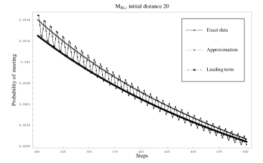
Figure 3: Left: Comparison of the meeting probability with the elliptic function estimation and the leading order term. The initial distance is set to 20 points. Right: Comparison of the meeting probability for the symmetric initial condition and zero initial distance with the estimation.

Let us now focus on the overall meeting probability defined by (34). In figure 4 we plot the overall probability that the two walkers will meet during the first $T=100$ steps.

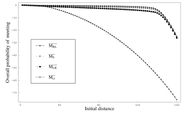
Figure 4: The overall probability of meeting for two distinguishable quantum and classical walker during first 100 steps as a function of the initial distance. Same plot on the log scale. Only the values for even points are plotted since for odd initial distance the walkers never meet.

On the first plot we present the difference between the three studied quantum situations, whereas the second plot, where the meeting probability is on the log scale, uncovers the difference between the quantum and classical random walk. In the log scale plot we can see that the overall meeting probability decays slower in the quantum case then in the classical case, up to to the initial distance of $\sqrt{2}T$. This can be understood by the shape and the time evolution of a single walker probability distribution. After $t$ steps the maximums of the probability distribution are around the point $s\pm\sqrt{2}t$, where $s$ is the initial starting point of the random walker. For $t=100$ steps the peaks are around the points $s\pm 140$. So when the two walkers are initially more then 140 points away, the peaks do not overlap, and the probability of meeting is given by just the tails of the single walker distributions, which have almost classical behavior. From the first plot we see that the overall meeting probability is broader in the quantum case compared to the classical, which drops down very fast. The numerical results in figure 5 show that the width of the overall meeting probability grows linearly with the upper bound T, the slope depends on the choice of the initial coin state. On the other hand in the classical case the width grows like $\sqrt{T}$.

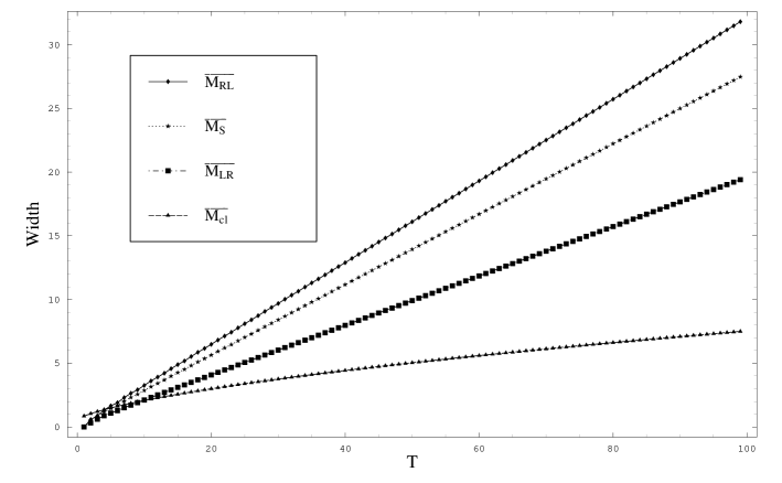
Figure 5: Width of the overall meeting probability as a function of the upper bound T.

Let us now analyze the overall meeting probability on a long time scale. In the Appendix A we show that in the classical case the overall meeting probability is approximately given by

$$\overline{M_{cl}}(T,d)\approx 1-\exp\left(-2\sqrt{\frac{T}{\pi}}\exp({-\frac{d^{2}}{T}})\right)\exp\left(2d\textrm{Erfc}(\frac{d}{\sqrt{T}})\right).$$ (49)

In the quantum case we consider $\ln{(1-\overline{M}_{D}(T,d))}$ ($M_{D}$ stands for all three particular quantum cases) and estimate it with the help of (3.1) by

$$\ln{(1-\overline{M}_{D}(T,d))} = \sum_{t=d}^{T}\ln{(1-M_{D}(t,d))}\approx-\sum_{t=d}^{T}M_{D}(t,d)$$ (50)

$$\approx -\int\limits_{\sqrt{2}d}^{T}M_{D}(t,d)dt.$$

Therefore we can estimate the overall meeting probability for $T>\sqrt{2}d$ by

$$\overline{M}_{D}(T,d)\approx 1-\exp\left(-\int\limits_{\sqrt{2}d}^{T}M_{D}(t,d)dt\right).$$ (51)

The meeting probability in the quantum case (3.1) involves elliptic integrals in a rather complicated form. However, we can estimate how fast the overall meeting probability converges to 1 for a fixed initial distance. This is determined by the rate at which the integral in (51) diverges. Before we proceed notice that

$$\int\limits_{\sqrt{2}d}^{\alpha d}M_{D}(t,d)dt=C(\alpha),$$ (52)

i.e. the integral does not depend on the initial distance $d$. For large $t$ we can estimate the meeting probability by (47) and thus we can divide the integral in (51) into

$$\int\limits_{\sqrt{2}d}^{T}M_{D}(t,d)dt \approx \int\limits_{\sqrt{2}d}^{\alpha d}M_{D}(t,d)dt+\frac{2\sqrt{2}}{\pi^{2}}\int\limits_{\alpha d}^{T}\frac{\ln{(\frac{2\sqrt{t}}{d})}}{t}dt$$ (53)

$$\approx C(\alpha)+\frac{\sqrt{2}}{\pi^{2}}\ln^{2}{\left(\frac{2\sqrt{2}T}{d}\right)},$$

for appropriately large $\alpha$. Therefore the exponent in (51) goes like $-\ln^{2}(T)$ for large $T$. On the other hand, in the classical case from the estimation (49) we obtain that the asymptotic behavior of the exponent is given $-\sqrt{T}$. Comparing these two we conclude that the overall meeting probability converges faster to one in the classical case.

To conclude, the quadratic speed-up of the width shown in figure 5 follows from the the quadratically faster spreading of the quantum random walk. On the other hand for large times the meeting probability decays faster in the quantum walk, which leads to the slower convergence of the overall meeting probability.

3.2 Effect of the entanglement for distinguishable walkers

We will now consider the case when the two distinguishable walkers are initially entangled. According to (23) the meeting probability is no longer given by the product of single walker probability distributions. However, it can be described using single walker probability amplitudes. We consider the initial state of the following form

$$|\psi(0)\rangle=|0,2d\rangle\otimes|\chi\rangle,$$ (54)

where $|\chi\rangle$ is one of the Bell states

$$|\psi^{\pm}\rangle = \frac{1}{\sqrt{2}}\left(|LR\rangle\pm|RL\rangle\right),$$

$$|\phi^{\pm}\rangle = \frac{1}{\sqrt{2}}\left(|LL\rangle\pm|RR\rangle\right).$$ (55)

Recalling the probability amplitudes $\psi^{L(R)}(m,t)$ we can write the probability distributions of the two random walkers (16) in the form

$$P_{\psi^{\pm}}(m,n,t)=\$$

$$\quad\frac{1}{2}\sum_{i,j=L,R}|\psi_{i}^{L}(m,t)\psi_{j}^{R}(n-2d,t)\pm\psi_{i}^{R}(m,t)\psi_{j}^{L}(n-2d,t)|^{2},$$

$$P_{\phi^{\pm}}(m,n,t)=\$$

$$\quad\frac{1}{2}\sum_{i,j=L,R}|\psi_{i}^{L}(m,t)\psi_{j}^{L}(n-2d,t)\pm\psi_{i}^{R}(m,t)\psi_{j}^{R}(n-2d,t)|^{2}.$$ (56)

The meeting probabilities are given by the sum of the diagonal terms in (3.2)

$$M_{\psi^{\pm}}(t,d)=$$

$$\frac{1}{2}\sum_{m}\left\{\sum_{i,j=L,R}|\psi_{i}^{L}(m,t)\psi_{j}^{R}(m-2d,t)\pm\psi_{i}^{R}(m,t)\psi_{j}^{L}(m-2d,t)|^{2}\right\},$$ (57)

$$M_{\phi^{\pm}}(t,d)=$$

$$\frac{1}{2}\sum_{m}\left\{\sum_{i,j=L,R}|\psi_{i}^{L}(m,t)\psi_{j}^{L}(m-2d,t)\pm\psi_{i}^{R}(m,t)\psi_{j}^{R}(m-2d,t)|^{2}\right\}.$$ (58)

The reduced density operators for both coins are maximally mixed for all four bell states (3.2). From this fact follows that the reduced density operators of the walkers are

$$\rho_{1}(t) = \frac{1}{2}\left(|\psi^{L}(t)\rangle\langle\psi^{L}(t)|+|\psi^{R}(t)\rangle\langle\psi^{R}(t)|\right)$$

$$\rho_{2}(t) = \frac{1}{2}\left(|\psi^{L}_{d}(t)\rangle\langle\psi^{L}_{d}(t)|+|\psi^{R}_{d}(t)\rangle\langle\psi^{R}_{d}(t)|\right),$$ (59)

where $|\psi^{L(R)}_{d}(t)\rangle$ are analogous to $|\psi^{L(R)}(t)\rangle$ but shifted by $2d$, i.e.

$$|\psi^{L(R)}(t)\rangle=\frac{1}{2}\sum_{m}\left(\psi^{L(R)}_{L}(m,t)|m,L\rangle+\psi^{L(R)}_{R}(m,t)|m,R\rangle\right)$$

$$|\psi^{L(R)}_{d}(t)\rangle=\$$

$$\frac{1}{2}\sum_{m}\left(\psi^{L(R)}_{L}(m-2d,t)|m,L\rangle+\psi^{L(R)}_{R}(m-2d,t)|m,R\rangle\right).$$ (60)

The reduced probabilities are therefore

$$P_{1}(m,t) = \frac{1}{2}(P^{L}(m,t)+P^{R}(m,t))$$

$$P_{2}(m,t) = P_{1}(m-2d,t),$$ (61)

which are symmetric and unbiased. Notice that the product of the reduced probabilities (3.2) gives the probability distribution of a symmetric case studied in the previous section. Therefore to catch the interference effect in the meeting problem we compare the random walks with entangled coin states (3.2) with the symmetric case $M_{S}$. The figure 6 shows the meeting probabilities and the difference $M_{\chi}-M_{S}$, the initial distance between the two walker was chosen to be 10 points.

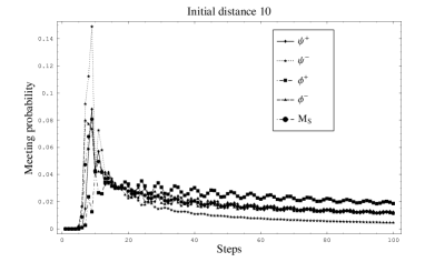
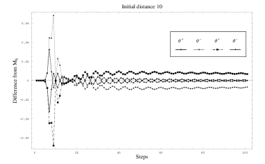
Figure 6: Comparison of the meeting probability for the initially entangled coins and the symmetric case. The difference in the meeting probability.

We see that the effect of the entanglement could be both positive or negative. Notice that

$$M_{\psi^{-}}(t,d)-M_{S}(t,d) = -\left(M_{\phi^{+}}(t,d)-M_{S}(t,d)\right)$$

$$M_{\phi^{-}}(t,d)-M_{S}(t,d) = -\left(M_{\psi^{+}}(t,d)-M_{S}(t,d)\right),$$ (62)

so the effect of $|\psi^{-}\rangle$ is opposite to $|\phi^{+}\rangle$ and $|\phi^{-}\rangle$ is opposite to $|\psi^{+}\rangle$. The main difference is around the point $t\approx\sqrt{2}d$, i.e., the point where for the factorized states the maximum of the meeting probability is reached. The peak value is nearly doubled for $M_{\psi^{-}}$ (note that for $M_{S}$ the peak value is given by (3.1), which for $d=10$ gives $\approx 0.063$), but significantly reduced for $M_{\phi^{+}}$. On the long time scale, however, the meeting probability $M_{\psi^{-}}$ decays faster than in other situations. According to the numerical simulations, the meeting probabilities for $|\psi^{+}\rangle$ and $|\phi^{\pm}\rangle$ maintain the asymptotic behavior $\ln{t}/t$, but for $|\psi^{-}\rangle$ it goes like

$$M_{\psi^{-}}(t,d)\sim\frac{1}{t}.$$ (63)

The initial entanglement between the walkers influences the height of the peaks giving the maximum meeting probability and affects also the meeting probability on the long time scale.

3.3 Indistinguishable walkers

Let us briefly comment on the effect of the indistinguishability of the walkers on the meeting probability. As an example, we consider the initial state of the walkers of the form $|1_{(0,R)}1_{(2d,L)}\rangle$, i.e. one walker starts at the site zero with the right coin state and one starts at $2d$ with left state. This corresponds to the case $M_{RL}$ for the distinguishable walkers. The meeting probabilities are according to (2.2), (31) given by

$$M_{B}(t,d) = \sum_{m}\{2|\psi_{L}^{R}(m,t)|^{2}|\psi_{L}^{L}(m-2d,t)|^{2}+$$

$$+2|\psi_{R}^{R}(m,t)|^{2}|\psi_{R}^{L}(m-2d,t)|^{2}+$$

$$+|\psi_{L}^{R}(m,t)\psi_{R}^{L}(m-2d,t)+$$

$$+\psi_{R}^{R}(m,t)\psi_{L}^{L}(m-2d,t|^{2}\}$$

$$M_{F}(t,d) = \sum_{m}\left(|\psi_{L}^{R}(m,t)\psi_{R}^{L}(m-2d,t)-\psi_{R}^{R}(m,t)\psi_{L}^{L}(m-2d,t)|^{2}\right).$$

In figure 7 we plot the meeting probabilities and the difference $M_{B,F}-M_{RL}$.

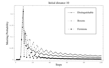
Figure 7: Comparison of the meeting probability for bosons, fermions and distinguishable walkers. The difference in the meeting probability.

From the figure we infer that the peak value is in this case only slightly changed. Significant differences appear on the long time scale. The meeting probability is greater for bosons and smaller for fermions compared to the case of distinguishable walkers. This behavior can be understood by examining the asymptotic properties of the expressions (3.3). Numerical evidence indicates that the meeting probability for bosons has the asymptotic behavior of the form $\ln(t)/t$. For fermions the decay of the meeting probability is faster having the form

$$M_{F}(t,d)\sim\frac{1}{t}.$$ (65)

The fermion exclusion principle simply works against an enhancement of the meeting probability.

4 Conclusions

We have defined and analyzed the problem of meeting in the quantum walk on an infinite line with two random walkers. For distinguishable walkers we have derived analytical formulas for the meeting probability. The asymptotic behavior following from these results shows that the meeting probability decays faster but not quadratically faster than in the classical random walk. This results in the slower convergency of the overall meeting probability. We have studied the influence of the entanglement and the indistinguishability of the walkers on the meeting probability. The influence is particularly visible for fermions and in the case of distinguishable walkers for the case of initial entangled singlet state.

Let us briefly comment on the correspondence between a one dimensional walk with two random walkers and a two dimensional walk. As two dimensional walks have been studied by many authors the possibility of common coin (i.e. a coin which is not a tensor product) for both walkers has arisen. In the context of one dimensional walk with two walkers this would mean some kind of interaction between the two walkers. It would be of interest to find coins which would attract the walkers and thus lead to an increase of the meeting probability, or repulsive coins with the opposite effect. Such interaction would be of infinite range as the walk will be driven by the same coin independent of the walkers distance. We can also think about local interactions where the walk is driven by a common coin for both walkers only when the distance between the walkers is smaller than some constant or they are at the same lattice point.

5 Acknowledgement

The financial support by GA ČR 202/04/2101, MŠMT LC 06001, the Czech-Hungarian cooperation project (CZ-2/2005,KONTAKT), by the Hungarian Scientific Research Fund (T043287 and T049234) and EU project QUELE is gratefully acknowledged.

References

Appendix A The meeting problem in the classical random walk

Let us define the meeting problem on the classical level. We assume two particles which in each step of the process can perform randomly a step to the left or to the right on a one dimensional lattice labeled by integers. Initial distance between the two walkers is $2d$, because for odd initial distance the two walkers never meet, due to the transitional invariance we can assume that one walker starts in the vertex labeled by 0 and the other one in the vertex $2d$. We assume complete randomness, i.e. the probabilities for the step right or left are equal. We ask for the probability that the two particles meet again after $t$ steps either at a certain position $m$ or we might ask for the total probability to meet (the sum of probabilities at all of the possible positions). Simple analysis reveals that the probability to meet at a certain position $m$ equals to

$$M_{cl}(t,m,d)=\frac{1}{2^{2t}}{t\choose\frac{t+m}{2}}{t\choose\frac{t+m-2d}{2}}.$$ (66)

The total probability that the two particles are reunited after $t$ steps reads

$$M_{cl}(t,d)=\sum\limits^{t}_{m=2d-t}\frac{1}{2^{2t}}{t\choose\frac{t+m}{2}}{t\choose\frac{t+m-2d}{2}},$$ (67)

which simplifies to

$$M_{cl}(t,d)=\frac{1}{2^{2t}}{2t\choose m+d}.$$ (68)

This function has a maximum for $t=2d^{2}$ of value

$$M_{cl}(2d^{2},d)=\frac{(4d^{2})!}{16^{d^{2}}(d(2d-1))!(d(2d+1))!}.$$ (69)

To obtain the asymptotic behavior of the meeting probability we approximate the one-walker probability distribution by a gaussian

$$P_{cl}(x,t,d)=\frac{1}{\sqrt{\pi t}}\exp(-\frac{(x-2d)^{2}}{2t}),$$ (70)

which leads to the following estimate on the meeting probability

$$M_{cl}(t,d)\approx\int\limits_{-\infty}^{+\infty}P_{cl}(x,t,0)P_{cl}(x,t,d)dx=\frac{1}{\sqrt{\pi t}}\exp(-\frac{d^{2}}{t}).$$ (71)

With the help of this estimation we can simplify the maximal probability of meeting into

$$M_{cl}(2d^{2},d)\approx\frac{1}{\sqrt{2\pi e}d}.$$ (72)

For a fixed initial distance $d$ we get the long-time approximation for $t>d^{2}$

$$M_{cl}(t,d)\approx\frac{1}{\sqrt{\pi t}}(1-\frac{d^{2}}{t}).$$ (73)

Finally we study the overall probability that the two walkers will meet at least once during first $T$ steps, which is given by

$$\overline{M_{cl}}(T,d)=1-\prod\limits^{T}_{k=d}{(1-M_{cl}(k,d))}.$$ (74)

To estimate this function we take the logarithm of $1-\overline{M_{cl}}(T,d)$ and use the first order of the Taylor expansion to obtain

$$ln{\left(1-\overline{M_{cl}}(T,d)\right)}=\sum_{k=d}^{T}ln{\left(1-M_{cl}(k,d)\right)}\approx-\sum_{k=d}^{T}M_{cl}(k,d).$$ (75)

From this with the help of the relation (68) we get the approximation of the overall meeting probability

$$\overline{M_{cl}}(T,d)\approx 1-\exp\left(-\sum_{k=d}^{T}\frac{1}{4^{k}}{2k\choose k+d}\right).$$ (76)

We estimate the sum in the exponential (76) by an integral with the help of the formula (71)

$$\sum_{k=d}^{T}\frac{1}{4^{k}}{2k\choose k+d} \approx \int\limits_{0}^{T}\frac{1}{\sqrt{\pi t}}\exp(-\frac{d^{2}}{t})dt$$ (77)

$$= 2\sqrt{\frac{T}{\pi}}\exp(-\frac{d^{2}}{T})-2d\textrm{Erfc}(\frac{d}{\sqrt{T}}),$$

where Erfc is the complementary error function

$$\textrm{Erfc}(x)=1-\textrm{Erf}(x)=1-\frac{2}{\pi}\int\limits_{0}^{x}e^{-t^{2}}dt.$$ (78)

With the help of the estimation (77) we obtain the approximation of the overall meeting probability

$$\overline{M_{cl}}(T,d)\approx 1-\exp\left(-2\sqrt{\frac{T}{\pi}}\exp({-\frac{d^{2}}{T}})\right)\exp\left(2d\textrm{Erfc}(\frac{d}{\sqrt{T}})\right).$$ (79)

References

- [1] R. Burioni and D. Cassi, J. Phys. A 38, R45 (2006)
- [2] Y. Aharonov, L. Davidovich, N. Zagury: Phys. Rev. A 48, 1687 (1993)
- [3] J. Kempe: Contemporary Physics, Vol. 44 (4), 307 (2003)
- [4] N. Shenvi, J. Kempe, K. B. Whaley, Phys. Rev. A. 67, 052307 (2003)
- [5] A. M. Childs, R. Cleve, E. Deotto, E. Fahri, S. Gutman, D. A. Spielman, Proc. 35th Symposium on the Theory of Computing (ACM Press, New York, 2003), p. 59
- [6] A. Nayak, A. Vishwanath: Quantum walk on a line, pre-print quant-ph/0010117
- [7] P. L. Knight, E. Roldán, J. E. Sipe: J. Mod. Opt. 51, 1761 (2004)
- [8] H. A. Carteret, M. E. H. Ismail, B. Richmond: J. Phys. A 36, 8775 (2003)
- [9] H. A. Carteret, B. Richmond, N. M. Temme: J. Phys. A 38, 8641 (2005)
- [10] C. A. Ryan, M. Laforest, J. C. Boileau, R. Laflamme: Phys. Rev. A 74, 062317 (2005)
- [11] G. S. Agarwal, P.K. Pathak: Phys. Rev. A 72, 033815 (2005)
- [12] M. Hillery, J. Bergou, E. Feldman: Phys. Rev. A 68, 032314 (2003)
- [13] H. Jeong, M. Paternostro, M. S. Kim, Phys. Rev. A 69, 012310 (2004)
- [14] D. Bouwmeester, I. Marzoli, G. P. Karman, W. Schleich and J. P. Woerdman, Phys. Rev. A 61, 01341 (1999)
- [15] B. C. Travaglione, G. J. Milburn, Phys. Rev. A 65, 032310 (2002)
- [16] W. Dür, R. Raussendorf, V. N. Kendon, H. J. Briegel, Phys. Rev. A 66, 052319 (2002)
- [17] K. Eckert, J. Mompart, G. Birkl, M. Lewenstein, Phys. Rev. A 72, 012327 (2005)
- [18] O. Mandel, M. Greiner, A. Widera, T. Rom, T. W. Hänsch, I. Bloch, Phys. Rev. Lett. 91, 010407 (2003)
- [19] E. Farhi, S. Gutman: Phys. Rev. A 58, 915 (1998)
- [20] T. D. Mackay, S. D. Bartlett, L. T. Stephenson and B. C. Sanders: J. Phys. A 35, 2745 (2002)
- [21] P. Törmä, I. Jex, W. P. Schleich Phys. Rev. A 65, 052110 (2002)
- [22] K. Lindberg, V. Seshadri, K. E. Shuler, G. H. Weiss: J. Stat. Phys. 23, 11 (1980)
- [23] Y. Omar, N. Paukovic, L. Sheridan, S. Bose: Quantum walk on a line with two entangled particles, quant-ph/0411065
- [24] B. Tregenna, W. Flanagan, R. Maile, V. Kendon: New Journal of Physics 5, 83.1 (2003)
- [25] M. Abramowitz, I. A. Stegun: Handbook of Mathematical Functions with Formulas, Graphs, and Mathematical Tables, Dover Publications 1972