Supercritical series expansion for the contact process in heterogeneous and disordered environments

Abstract

The supercritical series expansion of the survival probability for the one-dimensional contact process in heterogeneous and disordered lattices is used for the evaluation of the loci of critical points and critical exponents $\beta$. The heterogeneity and disorder are modeled by considering binary regular and irregular lattices of nodes characterized by different recovery rates and identical transmission rates. Two analytical approaches based on Nested Padé approximants and Partial Differential approximants were used in the case of expansions with respect to two variables (two recovery rates) for the evaluation of the critical values and critical exponents. The critical exponents in heterogeneous systems are very close to those for the homogeneous contact process thus confirming that the contact process in periodic heterogeneous environment belongs to the directed percolation universality class. The disordered systems, in contrast, seem to have continuously varying critical exponents.

I Introduction

In nonequilibrium statistical mechanics, phase transitions have been identified and studied for some time now. Similar to equilibrium systems, these phase transitions fall into a number of different universality classes, one of which is the directed percolation (DP) universality class Ódor (2004); Hinrichsen (2000). According to a conjecture by Janssen Janssen (1981) and Grassberger Grassberger (1982), all absorbing state phase transitions with a scalar order parameter and no additional conservation laws are characterized by DP critical exponents.

One of the questions that has not been answered conclusively is how the introduction of quenched disorder affects the universal critical behavior of the DP class. According to the Harris criterion Harris (1974a), the critical exponents should change even for weak disorder. This has been investigated in particular for the contact process (CP) Liggett (1985) which is one of the archetypical models of the DP universality class. Currently, there are two alternative scenarios how the exponents change with introduction of disorder: according to results in Refs. Moreira and Dickman (1996); Cafiero et al. (1998); Dickman and Moreira (1998); Hooyberghs et al. (2003, 2004), they change continuously with degree of disorder, while Vojta Vojta and Dickison (2005) has suggested an abrupt change to the values in the strong disorder limit corresponding to the universality class of the random transverse Ising model.

The above controversy can be addressed either by numerical or analytical methods. Among analytical methods, time-dependent perturbation theory as introduced by Dickman and Jensen Dickman and Jensen (1991); Jensen and Dickman (1993) for homogeneous $1d$ systems gives the most accurate numerical values. Technically, this has been done by using one-variable Padé approximants in the analysis of the series for the survival probability. In this paper, we extend their approach to heterogeneous and disordered $1d$ lattices and introduce the use of a Padé approximants similar to the Nested Padé approximants (NPA’s) Guillaume (1997); Guillaume and Huard (2000) in order to deal with two control parameters (two recovery rates), characteristic of binary lattices. A different approach based on partial differential approximants (PDA’s) has been used by Dantas and Stilck in Ref. Dantas and Stilck (2005), who applied the supercritical series expansion to study the crossover between the $1d$ CP and the voter model Liggett (1985), thereby introducing a second control parameter to the perturbation theory. We also use PDA’s in order to compare results from the two extrapolation methods.

The aim of the paper is two-fold: first, we present and discuss the technical details of the supercritical series expansions in the case of two variables, i.e. of two different recovery rates characteristic of nodes of two different types, which are different from the well-studied one-parameter case Dickman and Jensen (1991); Jensen and Dickman (1993). Second, we investigate the range of applicability and the effects of variations of our procedure based on NPA’s on the estimates of critical values and exponents and compare these results to those obtained by employing PDA’s.

The structure of the paper is as follows: we introduce the CP in Sec. II. The supercritical series expansion, the analysis of the resulting two-variable series and the configurational averaging of the order parameter for disordered environments are discussed in Sec. III. In Sec. IV, we present the results in terms of phase diagrams and the critical exponent $\beta$ for the different systems, which we then discuss in the last Sec. V.

II Model

The CP, originally introduced by Harris Harris (1974b), is a spatial SIS (Susceptible-Infected-Susceptible)-model for the spread of epidemics through a network. In a network, usually taken to be a hyper-cubic lattice, the nodes or sites can be in one of two states: “infected” or “susceptible”. A susceptible/vacant site $i$ can be infected by a neighboring infected/occupied site $j$, while an occupied site $k$ can spontaneously recover and become susceptible again. These processes occur with rates $\lambda_{ij}/z$ and $\mu_{k}$, respectively, where $z$ is the number of nearest neighbors in the lattice.

In all dimensions, the CP undergoes a nonequilibrium phase transition into an absorbing state which does not allow any further time evolution. For a fixed set of transmission rates, this occurs when the recovery rates become smaller than a set of critical values. At this point, the survival probability, that is the probability that process will not enter the absorbing state (in the thermodynamic limit), becomes greater than zero. Several observables can be identified that describe the critical state of the CP, such as the average density of infected sites, $\rho\,(t)$, or the survival probability up to time $t$ after starting from a single seed, $P_{\text{s}}\,(t)$. As $t\to\infty$, in a homogeneous system ($\lambda_{ij}=1$ and $\mu_{k}=\mu$), close to the critical point these quantities are expected to behave like Hinrichsen (2000)

$$\lim_{t\to\infty}\rho(t)\equiv\rho_{\text{stat}}\sim\Delta^{\beta}\qquad\lim_{t\to\infty}P_{\text{s}}(t)\equiv P_{\infty}\sim\Delta^{\beta}.$$ (1)

Here $\beta$ is the critical exponent associated with stationary behavior of the order parameter and $\Delta=\mu_{c}-\mu>0$, where $\mu_{c}$ is the critical point for the control parameter recovery rate $\mu$.

Each site $i$ of the system of $N_{\text{s}}$ nodes obeying the rules of the CP can be in two states: $|\sigma_{i}\rangle$ where $\sigma_{i}=0$ or $\sigma_{i}=1$ so that a microstate of the system with $N_{\text{s}}$ sites can be written as

$$\mbox{$|\sigma\rangle$}=\mbox{$|\sigma_{1}\rangle$}\otimes\ldots\otimes\mbox{$|\sigma_{N_{\text{s}}}\rangle$}=\bigotimes_{i}^{N_{\text{s}}}\mbox{$|\sigma_{i}\rangle$}=\bigotimes_{i}^{N_{\text{s}}}\left(\begin{array}[]{c}1-\sigma_{i}\\ \sigma_{i}\end{array}\right)$$

This representation ensures that the microstate vectors form a $2^{N_{\text{s}}}$-dimensional orthonormal basis. The state of the system at time $t$ is

$$\mbox{$|P(t)\rangle$}=\sum_{\sigma}P(\sigma,t)\,\mbox{$|\sigma\rangle$}$$ (3)

where $P(\sigma,t)=\mbox{$\langle\sigma|P(t)\rangle$}$ is the probability that the system is found in microstate $|\sigma\rangle$. The time-evolution of the state of the system is governed by the master equation

$$\partial_{t}\mbox{$|P(t)\rangle$}=\hat{L}\mbox{$|P(t)\rangle$}$$ (4)

where $\hat{L}$ is the Liouville operator whose non-zero off-diagonal elements in this basis are the transition rates between microstates that for the CP differ in their occupation number by one. This operator describes the probability flow between different microstates and is thus represented by a stochastic matrix in which all the diagonal elements are the sums of the off-diagonal elements in the corresponding columns taken with the opposite sign.

In a formalism introduced by Doi Doi (1976) and Peliti Peliti (1985) for stochastic systems, “annihilation” and “creation” operators on site $i$, $a_{i}^{\phantom{\dagger}}$ and $a_{i}^{\dagger}$, respectively, are defined, such that $\mbox{$a_{i}^{\phantom{\dagger}}$}\,\mbox{$|\sigma_{i}\rangle$}=\sigma_{i}\,\mbox{$|\sigma_{i}-1\rangle$}$ and $\mbox{$a_{i}^{\dagger}$}\,\mbox{$|\sigma_{i}\rangle$}=(1-\sigma_{i})\,\mbox{$|\sigma_{i}+1\rangle$}$ (e.g. $\mbox{$a_{i}^{\phantom{\dagger}}$}\mbox{$|0\rangle$}=0$) and that they obey hard-core bosonic commutation relations.

For simplicity, we assume all the transmission rates to be the same and define the time scale by setting $\lambda_{ij}=1$. The recovery rates for binary systems are characterized by one of two values $\mu_{i}=\{\mu_{A},\mu_{B}\}$. For such models, the operator $\hat{L}$ in the one-dimensional case reads as

$$\hat{L}=\mu\,\hat{W}+\hat{V}~{},$$ (5)

where the operators $\mu\,\hat{W}$ and $\hat{V}$ are

$$\mu\,\hat{W} = \mu\sum_{i}\frac{\mu_{i}}{\mu}\,(1-\mbox{$a_{i}^{\dagger}$})\,\mbox{$a_{i}^{\phantom{\dagger}}$}~{},$$ (6)

$$\hat{V} = \sum_{i}\frac{1}{2}\,(1-\mbox{$a_{i}^{\phantom{\dagger}}$})\,\mbox{$a_{i}^{\dagger}$}\,(\mbox{$a_{i-1}^{\dagger}$}\mbox{$a_{i-1}^{\phantom{\dagger}}$}+\mbox{$a_{i+1}^{\dagger}$}\mbox{$a_{i+1}^{\phantom{\dagger}}$})~{}.$$ (7)

The parameter $\mu$ is introduced for convenience and $\mu_{i}/\mu\sim 1$ with both recovery rates being close to the homogeneous critical point and thus $\mu_{i}\lesssim 1$. The operator $\hat{V}$ creates offspring at the nearest neighbors of an occupied sites, while $\hat{W}$ destroys occupation at sites. The above formalism is useful for the supercritical series expansion in $\mu$ described below.

III Analysis

III.1 Supercritical Series Expansion

The supercritical series expansion is a perturbation series for the ultimate survival probability $P_{\infty}$ which is taken to be the order parameter, with $P_{\infty}>0$ being characteristic of the CP in the active phase. To probe the long-time limit of the system, the Laplace transform of the probability state vector is taken,

$$\mbox{$|\tilde{P}\,(s)\rangle$}=\int_{0}^{\infty}dt\,e^{-st}\,\mbox{$|P\,(t)\rangle$}~{},$$ (8)

so that a standard identity of Laplace-transform theory, $\lim_{t\rightarrow\infty}f(t)=\lim_{s\rightarrow 0}s\,\tilde{f}(s)$, can be used. The ultimate survival probability is then given by

$$P_{\infty}=\lim_{s\rightarrow 0}\left(1-s\,\mbox{$\langle 0|\tilde{P}\,(s)\rangle$}\right)~{}.$$ (9)

Inserting the formal solution $\mbox{$|P\,(t)\rangle$}=e^{-\hat{L}\,t}\mbox{$|P\,(0)\rangle$}$ of Eq. (4) into Eq. (8) results in

$$\mbox{$|\tilde{P}\,(s)\rangle$}=(s-\mu\,\hat{W}-\hat{V})^{-1}\mbox{$|P\,(0)\rangle$}~{}.$$ (10)

We can then formally expand the operator on the right hand-side of Eq. (10) in a Taylor series with respect to the small parameter $\mu$ thus obtaining the following supercritical expansion

$$|\tilde{P}\,(s)\rangle = \mbox{$|\widetilde{P}_{0}(s)\rangle$}+\mu\mbox{$|\widetilde{P}_{1}(s)\rangle$}+\mu^{2}\mbox{$|\widetilde{P}_{2}(s)\rangle$}+\ldots$$ (11)

where the vectors $|\widetilde{P}_{n}(s)\rangle$ obey the following recursion relations:

$$|\widetilde{P}_{0}(s)\rangle = (s-\hat{V})^{-1}\mbox{$|P(0)\rangle$}$$ (12)

$$|\widetilde{P}_{n}(s)\rangle = (s-\hat{V})^{-1}\hat{W}\mbox{$|\widetilde{P}_{n-1}(s)\rangle$}\quad\mbox{for}~{}n\geq 1~{}.$$ (13)

The action of the operator $\hat{W}$ on a given configuration can be straightforwardly computed using its definition given by Eq. (6), i.e.

$$\hat{W}\mbox{$|\sigma\rangle$}=\sum_{i}^{m}\frac{\mu_{i}}{\mu}\left(\mbox{$|\overline{\sigma}^{i}\rangle$}-\mbox{$|\sigma\rangle$}\right).$$ (14)

The summation is taken over all $m$ occupied sites in state $\sigma$ and $\mbox{$|\overline{\sigma}^{i}\rangle$}=\mbox{$a_{i}^{\phantom{\dagger}}$}\mbox{$|\sigma\rangle$}$, i.e. the $\overline{\sigma}^{i}$ and $\sigma$ have the same occupation except for site $i$ being occupied in state $\sigma$ and vacant in $\overline{\sigma}^{i}$.

The action of the operator $(s-\hat{V})^{-1}$ on a given configuration, $|\sigma\rangle$, can be computed with the use of the following identity,

$$(s-\hat{V})^{-1}=s^{-1}+s^{-1}(s-\hat{V})^{-1}\hat{V}~{},$$ (15)

so that

$$(s-\hat{V})^{-1}\mbox{$|\sigma\rangle$}=\frac{1}{s+q_{1}/2+q_{2}}\left(\mbox{$|\sigma\rangle$}+(s-\hat{V})^{-1}\left[\frac{1}{2}\sum_{i}^{q_{1}}\mbox{$|\tilde{\sigma}^{1,i}\rangle$}+\sum_{i}^{q_{2}}\mbox{$|\tilde{\sigma}^{2,i}\rangle$}\right]\right)$$ (16)

where the sums represent the action of the operator $\hat{V}$ on the state $\sigma$ with vacant sites of two types: sites which have one (first sum in Eq. (16) is taken over a number $q_{1}$ of such sites) or two (second sum in Eq. (16) is taken over $q_{2}$ of such sites) occupied nearest neighbors. The vectors $|\overline{\sigma}^{1,i}\rangle$ and $|\overline{\sigma}^{2,i}\rangle$ represent the states in which the formerly vacant sites $i$ of the first and second type, respectively, are now occupied. To go further we should use the recursive nature of the operator $(s-\hat{V})^{-1}$ and substitute its representation given by Eq. (15) into Eq. (16). Such a procedure can generate an infinite number of new configurations. However, when we calculate the survival probability perturbatively up to a given order $N$ in $\mu$ for the initial condition of a single occupied site, it is only necessary to retain states with up to $N$ occupied sites. This is due the fact that the annihilation operator $\hat{W}$ in an expansion up to order $\mu^{N}$ acts $N$ times on any generated state, after which remaining states will be projected onto the absorbing state, thereby projecting out any states with more than $N$ occupied sites. Following this procedure, we can perturbatively calculate the survival probability $P_{\infty}$ and thus find the critical point where the survival probability becomes zero. In order to obtain good numerical estimates of this critical value and compute critical exponents, it is necessary to employ numerical methods such as Padé approximants Baker and Graves-Morris (1996).

III.2 Nested Padé Approximants: Critical Values and Exponent

For systems with two different recovery rates, $\mu_{A}$ and $\mu_{B}$, the survival probability (see Eq. (9)) expanded in series is a polynomial in these two variables,

$$\mbox{$P_{\infty}$}(\mu_{A},\mu_{B})=1-\sum_{n=1}^{N}\sum_{m=0}^{n}~{}c_{nm}~{}\mu_{B}^{m}~{}\mu_{A}^{n-m}~{}.$$ (17)

The critical line $\mu_{B}^{(\text{c})}=\mu_{B}^{(\text{c})}(\mu_{A}^{(\text{c})})$ that separates the absorbing state from the active state is a solution to the equation $\mbox{$P_{\infty}$}(\mu_{A},\mu_{B})=0$ corresponding to the smallest (real) root. In practice, just finding the roots of the polynomial – the truncation of an infinite series at finite order – does not produce very good estimates of the critical values. Better results are obtained by using d-log Padé approximants Guttmann (1989): given an expansion in one variable, $\mbox{$P_{\infty}$}(\mu)$, up to order $N$, the Padé approximant Bender and Orszag (1978); Baker and Graves-Morris (1996) of the a series for $\partial_{\mu}\ln\mbox{$P_{\infty}$}(\mu)$ is formed. Technically, this is done by expanding the denominator of $\partial_{\mu}\ln\mbox{$P_{\infty}$}(\mu)=\partial_{\mu}P(\mu)/P(\mu)$ up to order $N-1$ and thus obtaining a polynomial $f_{N-1}(\mu)$ for this fraction, the Padé approximant of which is then constructed. The first positive (real) pole and its residue then provide good estimates of the critical value and the critical exponent of $P_{\infty}$, respectively. The extension of this approach to two variables, however, is not straightforward – there is a number of different multi-variable generalizations Chisholm (1973); Fisher and Kerr (1977) of the one-variable Padé approximation. In this work, we employ a scheme similar to the NPA’s Guillaume (1997); Guillaume and Huard (2000) in which we in turn form one-variable Padé approximants with respect to the two variables.

To this end, we transform the variables $(\mu_{A},\mu_{B})$ to the following three more convenient sets, T1, T2 and T3. The first transformation, T1, is symmetric so that the values $(\mu_{A},\mu_{B})$ are replaced by $(\bar{\mu},\delta)$ where $\bar{\mu}=(\mu_{A}+\mu_{B})/2$ and $\delta=(\mu_{A}-\mu_{B})/2$. The transformations T2 and T3 are asymmetric with $(\mu_{A},\mu_{B})$ replaced by either $(\bar{\mu}=\mu_{A},\delta=\mu_{A}-\mu_{B})$ or $(\bar{\mu}=\mu_{B},\delta=\mu_{B}-\mu_{A})$, respectively. Expanding $\frac{\partial}{\partial\bar{\mu}}\ln\mbox{$P_{\infty}$}(\bar{\mu},\delta)=\partial_{\bar{\mu}}\mbox{$P_{\infty}$}/\mbox{$P_{\infty}$}(\bar{\mu},\delta)$ up to order $N-1$ in $\bar{\mu}$ and $\delta$, we obtain

$$\frac{\partial}{\partial\bar{\mu}}\ln\mbox{$P_{\infty}$}(\bar{\mu},\delta)=\sum_{n=0}^{N-1}f_{n}(\delta)\bar{\mu}^{n}+O(\bar{\mu}^{N}).$$ (18)

We then form the Padé approximants of the coefficients,

$$f_{n}(\delta)=\frac{\sum_{m=0}^{J}q_{m}\delta^{m}}{1+\sum_{m=1}^{K}q_{J+m}\delta^{m}},$$ (19)

where $N-1-n=J+K$. As always with Padé approximants, we have the freedom to choose $J$ and $K$ for a given $n$. For even $N-1-n$, we use diagonal Padé approximants $[J,J]$ with $J=K=(N-1-n)/2$, while for odd $N-1-n$, we form approximants $[J-1,J]$ with $J=(N-n)/2$.

Then, in turn, we form the Padé approximant with respect to $\bar{\mu}$,

$$\partial_{\bar{\mu}}\ln\mbox{$P_{\infty}$}=\frac{\sum_{n=0}^{L}r_{n}(\delta)\,\bar{\mu}^{n}}{1+\sum_{n=1}^{M}r_{L+n}(\delta)\,\bar{\mu}^{n}}+O(\bar{\mu}^{N})$$ (20)

where $N-1=L+M$. A more graphical representation of the scheme is the following:

$$\partial_{\bar{\mu}}\ln\mbox{$P_{\infty}$} = \underbrace{(a_{0,0}+a_{0,1}\delta+\ldots+a_{0,N-1}\,\delta^{N-1})}+\underbrace{(a_{1,0}+\ldots a_{1,N-1}\,\delta^{N-2})}\bar{\mu}+\ldots a_{N-1,0}\,\bar{\mu}^{N-1}+O(\bar{\mu}^{N})$$ (21)

$$= \underbrace{\quad\big{[}\mbox{$\lfloor(N-1)/2\rfloor$},\mbox{$\lceil(N-1)/2\rceil$}\big{]}_{\delta}\hskip 13.0pt+\big{[}\mbox{$\lfloor(N-3)/2\rfloor$},\mbox{$\lceil(N-1)/2\rceil$}\big{]}_{\delta}\,\bar{\mu}+\ldots a_{N-1,0}\,\bar{\mu}^{N-1}}+O(\bar{\mu}^{N})$$ (22)

$$= \hskip 110.0pt\big{[}\mbox{$\lfloor(N-1)/2\rfloor$},\mbox{$\lceil(N-1)/2\rceil$}\big{]}_{\bar{\mu}}+O(\bar{\mu}^{N})$$ (23)

Here we have denoted the formation of the Padé approximant with respect to a variable $x$ with numerator degree $N$ and denominator degree $M$ as $\big{[}N,M\big{]}_{x}$ ($\lfloor\cdot\rfloor$ and $\lceil\cdot\rceil$ are the floor and ceiling functions, respectively).

Thus for any given $\delta$, we can find the corresponding pole of $\partial_{\bar{\mu}}\ln\mbox{$P_{\infty}$}(\bar{\mu},\delta)$, which is then taken to as the critical value $\bar{\mu}^{(\text{c})}(\delta)$, yielding a point on the critical line, $(\mu_{A}^{(\text{c})}=\bar{\mu}^{(\text{c})},\mu_{B}^{(\text{c})}=\bar{\mu}^{(\text{c})}+\delta)$, $(\mu_{A}^{(\text{c})}=\bar{\mu}^{(\text{c})}+\delta,\mu_{B}^{(\text{c})}=\bar{\mu}^{(\text{c})})$ or $(\mu_{A}^{(\text{c})}=\bar{\mu}^{(\text{c})}+\delta,\mu_{B}^{(\text{c})}=\bar{\mu}^{(\text{c})}-\delta)$, depending on the initial transformation.

It turns out that occasionally the first positive real roots are unphysical ones that appear before the physical solution. However, these roots are very closely matched by roots of the numerator of the Padé approximant of $\partial_{\bar{\mu}}\ln\mbox{$P_{\infty}$}(\mu_{A},\delta)$, so that these two cancel each other, leaving the physical root as the solution. In order to extract unphysical roots a further parameter $\gamma$ has been introduced. Two roots, $x_{1}$ and $x_{2}$, of the numerator, $n(x)$, and the denominator, $d(x)$, respectively, i.e. $(x-x_{1})n(x)/\left((x-x_{2})d(x)\right)$, are considered to be the same value and cancel if $|x_{1}-x_{2}|<\gamma$. All results presented below are obtained by setting $\gamma=10^{-3}$.

In order to evaluate the stability of a certain pole, several approximants are formed with respect to $\bar{\mu}$ close to the diagonal approximant, e.g. for even $N-1=2K$, we compute $[K,K],[K-1,K],[K,K-1],\ldots[K-2,K-2]$ and take the average over these poles. Once we obtained the critical value, the critical exponent $\beta$ associated with the order parameter $P_{\infty}$ can be found as well, as it is just the residue at the pole $\bar{\mu}^{(\text{c})}$. Again, the average over the residues for different Padé approximants is taken. As the error that we could extract from employing this method is small and does not take into account the inherent error in the series expansion, we perform this averaging to minimize the effects due to a particular choice of approximant and use the standard deviation only to evaluate the numerical stability of a pole.

III.3 Partial Differential Approximants: Critical Values

Another method for estimating critical values given a finite two-variable series are the PDA’s originally developed by Fisher Fisher (1977) in order to investigate multicritical points.

The starting point of this method is that one is given a finite two-variable polynomial, $F(x,y)=\sum_{(i,j)\in\mathbf{S}}f_{ij}x^{i}y^{j}$, that approximates a true function $f(x,y)$, that is expected to have the following form,

$$f(x,y)=((x-x_{c})+\alpha(y-y_{c}))^{\beta}\phi(x,y)$$ (24)

where $\phi(x,y)$ is some general function with $\phi(x_{c},y_{c})\neq 0$. The set $\mathbf{S}$ is a so-called label set that contains the pairs of powers $(i,j)$ of $x$ and $y$ only if $f_{ij}\neq 0$, i.e. $(i,j)\in\mathbf{S}$ if $F(x,y)$ has a non-zero term of order $x^{i}y^{j}$. For fixed label sets $\mathbf{L}$, $\mathbf{M}$ and $\mathbf{N}$, it is possible to find polynomials $P_{\mathbf{L}}(x,y)=\sum_{(i,j)\in\mathbf{L}}p_{ij}x^{i}y^{j}$, $Q_{\mathbf{M}}(x,y)=\sum_{(i,j)\in\mathbf{M}}q_{ij}x^{i}y^{j}$ and $R_{\mathbf{N}}(x,y)=\sum_{(i,j)\in\mathbf{N}}r_{ij}x^{i}y^{j}$ such that they satisfy the defining equation

$$P_{\mathbf{L}}(x,y)F=Q_{\mathbf{M}}(x,y)\frac{\partial F}{\partial x}+R_{\mathbf{N}}(x,y)\frac{\partial F}{\partial y}+E_{\mathbf{K}}(x,y)$$ (25)

with $E_{\mathbf{K}}=\sum_{(i,j)\notin\mathbf{K}}e_{ij}x^{i}y^{j}$ denoting a sum of non-zero terms whose powers are not in the matching set $\mathbf{K}$. This matching set defines for which powers $x^{i}y^{j}$ Eq. (25) should hold exactly with $e_{ij}=0$, while for $(m,n)\notin\mathbf{K}$, the values of $e_{mn}$ are allowed to be non-zero. In order for Eq. (25) to be a solvable set of linear equations, the label sets must obey the constraint that the label sets $\mathbf{L}$, $\mathbf{M}$ and $\mathbf{N}$ must together contain one more element than the matching set $\mathbf{K}$ because of the conventional choice of $p_{00}=1$.

Once the polynomials $P_{\mathbf{L}}$, $Q_{\mathbf{M}}$ and $R_{\mathbf{N}}$ are found, e.g. by using an algorithm proposed by Styer Styer (1990), they can be used to find an estimate for the line of critical points by the method of characteristics (e.g. see Stilck and Salinas (1981)). According to this method, consider a single curve of points which only depends on a single parameter $\tau$, $\mathbf{x}(\tau)=(x(\tau),y(\tau))$. The rate of change of $F(x(\tau),y(\tau))$ along this line is $\mathrm{d}F/\mathrm{d}\tau=(\partial F/\partial x)(\mathrm{d}x/\mathrm{d}\tau)+(\partial F/\partial y)(\mathrm{d}y/\mathrm{d}\tau)$. The survival probability $P_{\infty}$, for which we are going to apply this method, is zero along the critical line. Thus, considering the case where $F(x(\tau),y(\tau))=0$, it can be seen that the curve described by the equations

$$\frac{\mathrm{d}x}{\mathrm{d}\tau} = Q_{\mathbf{M}}(x(\tau),y(\tau))$$ (26)

$$\frac{\mathrm{d}y}{\mathrm{d}\tau} = R_{\mathbf{N}}(x(\tau),y(\tau))$$ (27)

and substituted in Eq. (25) yields the relation $0=(\partial F/\partial x)(\mathrm{d}x/\mathrm{d}\tau)+(\partial F/\partial y)(\mathrm{d}y/\mathrm{d}\tau)$. Together with a suitable initial condition, this curve is therefore equivalent to the critical line as $F$ does not change along the curve $\mathbf{x}(\tau)$. This suitable initial condition has to be a known point on the critical line: in our case, this is the critical point of the homogeneous system at which $x=y=x_{c}$.

III.4 Configurational Averaging

The schemes above are straightforwardly applied to heterogeneous topologically ordered systems. In topologically disordered systems, the survival probability has to be averaged over different realizations of disorder. For concreteness, we consider disorder only in recovery rates $\mu_{i}$ on different nodes $i$ assuming that $\mu_{i}$ are independent random variables distributed according to the probability distribution functions $\rho(\mu_{i})$. A configurationally averaged survival probability is then given by the following expression, $\langle\mbox{$P_{\infty}$}\rangle=\int\mbox{$P_{\infty}$}(\mu_{i})\prod_{i}\rho\,(\mu_{i})\text{d}\mu_{i}$. For simplicity, we consider a bimodal distribution of recovery rates,

$$\rho\,(\mu_{i})=p\,\delta(\mu_{i}-\mu_{A})+(1-p)\,\delta(\mu_{i}-\mu_{B})~{},$$ (28)

i.e. the nodes $A$ (hosts), characterized by recovery rate $\mu_{A}$, of concentration $p$ and $B$ (impurities) of concentration $1-p$ are randomly and independently placed on the sites of a regular chain.

Using the series expansion of order $N$ for $P_{\infty}$ is equivalent to considering the CP on the finite chain of length $2N-1$, i.e. for a given value of $n\leq N$ all states on $2n-1$ sites with the origin at its center with at most $n$ sites occupied contribute, so that

$$\langle\mbox{$P_{\infty}$}\rangle=1+\sum_{n=1}^{N}\sum_{m=0}^{n}\,\langle c_{nm}\rangle\,\mu_{B}^{m}\,\mu_{A}^{n-m}$$ (29)

where

$$\langle c_{nm}\rangle=\sum_{k=0}^{2n-1}\sum_{\{\mathbf{c}:\,N_{B}(\mathbf{c})=k\}}(1-p)^{k}p^{2n-1-k}c_{nm}(\mathbf{c})$$ (30)

with the second sum running over all disorder configurations $\mathbf{c}=(\mu_{-n+1},\ldots,\mu_{0},\ldots,\mu_{n-1})$ that have a certain number $N_{B}(\mathbf{c})$ of impurity sites $B$. The values of $c_{nm}$ are the coefficients in the expansion of the survival probability for a particular disorder configuration. The factor $(1-p)^{k}p^{2n-1-k}$ stems from the fact that the probability of having a particular disorder configuration is just the product of the probabilities of any site being either $\mu_{A}$ or $\mu_{B}$, drawn from the bimodal distribution given by Eq. (28).

The memory requirements in calculations of the coefficients in the series expansions impose a restriction, $N\leq N_{\text{max}}$, on the highest order of expansion for disordered lattices, $N_{\text{max}}=19$, which is rather lower than for homogeneous Jensen and Dickman (1993) and heterogeneous cases, $N_{\text{max}}=24$. The exact configurational averaging discussed above, exploiting symmetry about the origin and under the exchange of $\mu_{A}$ and $\mu_{B}$, is not possible for such high orders due to computational cost when dealing with a very large number (of $O(2^{2N_{\text{max}}})$) of configurations. We have been able to undertake the exact configurational averaging up to order $N_{\text{c,max}}=12$.

For higher orders, $N_{\text{c,max}}\leq N\leq N_{\text{max}}$, a configurationally averaged survival probability is calculated approximately by only including disorder configurations that have no more than a certain number of impurities in the averaging. Assuming that each coefficient is of the order of the coefficient in a homogeneous system, $c_{nm}(\mathbf{c})\sim c_{n}$, then each coefficient $\langle c_{nm}\rangle$ will remain of the same order of magnitude if we choose a maximum number of impurities $k_{\text{max}}(n,p)$ in

$$\langle c_{nm}\rangle\sim c_{n}\sum_{k=0}^{k_{\text{max}}}{2n-1\choose k}(1-p)^{k}p^{2n-1-k}$$ (31)

such that the sum is close to unity. For $(1-p)\ll 1$ and large $n\gg 1$, one can choose $k_{\text{max}}\ll 2n-1$, e.g. for $k_{\text{max}}(19,0.96)=2$, $\sum_{k=0}^{k_{\text{max}}}{2n-1\choose k}(1-p)^{k}p^{2n-1-k}=0.817$. For lower orders, the weight of the configurations that are dropped decreases for constant $k_{\text{max}}$, but, because it becomes computationally feasible, we choose to increase $k_{\text{max}}$ by one for each lower order by letting $k_{\text{max}}(N_{\text{max}}-i,p)=i+2$. This way, the lower the order the closer the approximate configurational averaging is to the exact one. With $k_{\text{max}}(N_{\text{max}}-i,p)=i+2$, the averaging becomes exact from order $n\leq N/3+1$.

IV Results

In this section, we will present the results for critical values and critical exponents obtained by the analysis described above and applied to different systems. These results come in the form of phase diagrams in which the critical points are plotted in the rate-space plane $(\mu_{A},\mu_{B})$ or as plots of the critical exponent $\beta$ as a function of the critical rate $\mu_{A}^{(\text{c})}$.

In Ref. Neugebauer et al. (2006), it has been demonstrated that for the $1d$ CP the line of critical points close to the homogeneous critical point, $(\mu_{A}=\mu_{\text{c}},\mu_{B}=\mu_{\text{c}})$ is well described by the relation

$$\mu_{\text{c}}\simeq\exp\left(\mathrm{E}[\ln(\mu_{i})]\right)~{},$$ (32)

where $\mathrm{E}[\cdot]$ denotes the expectation value with respect to the distribution of the recovery rates $\mu_{i}$. In this work, we will compare the critical points to the line given by Eq. (32) to examine how far from the homogeneous critical point the relationship describes the critical line well.

In all figures below, we only keep critical points and critical exponents that have a standard deviations from the mean values of less than $0.001$ and $0.005$, respectively, after averaging over the Padé approximants as described in Sec. III.2.

IV.1 Periodic Lattices

Figure 1: (Color online) Comparison of critical points (a) and critical exponents (b) of the $AB$ system obtained from series expansion for different orders $N$: $N=10$ ($\circ$), $N=17$ ($\diamond$) and $N=24$ ($+$). The symmetric transformation T1 was used. The dashed lines (     ) are given by Eq. (32) in (a) and by $\beta$ at the homogeneous critical point, $\beta=0.2769$, from series expansions Jensen and Dickman (1993) for the CP, in (b).

Figure 2: (Color online) Comparison of the critical points (a) and critical exponents (b) of the $AB$ system obtained from series expansions up to order $N=24$ with different transformations, T1 ($\circ$) and T2 ($+$). The dashed lines (     ) are given by Eq. (32) in (a) and by $\beta$ at the homogeneous critical point, $\beta=0.2769$, from series expansions Jensen and Dickman (1993) for the CP, in (b).

Figure 3: (Color online) Comparison of the critical values (a) and critical exponents $\beta$ (b) of the $AAB$ system obtained from series expansions up to order $N=24$ with different transformations, T1 ($\circ$), T2 ($+$) and T3 ($\diamond$). The dashed lines (     ) are given by Eq. (32) in (a) and by $\beta$ at the homogeneous critical point, $\beta=0.2769$, from series expansions Jensen and Dickman (1993) for the CP, in (b).

Figure 4: (Color online) Comparison of critical values (a) and critical exponents (b) of the $AAB$ lattice obtained from series expansions up to overall order $N=24$ which are cut off at order $M=12$ ($+$) or in which all the terms up to order $M=23$ ($\circ$) are retained. Transformation T2 was used to obtain these critical points. The dashed lines (     ) are given by Eq. (32) in (a) and by $\beta$ at the homogeneous critical point, $\beta=0.2769$, from series expansions Jensen and Dickman (1993) for the CP, in (b).

Figure 5: (Color online) Comparison of critical values (a) and critical exponents (b) of the $AB$ lattice obtained from series expansions up to overall order $N=24$ which are cut off at order $M=12$ ($+$) or in which all the terms up to order $M=23$ ($\circ$) are retained. Transformations T2 and T1, respectively, were used to obtain these critical points. The dashed lines (     ) are given by Eq. (32) in (a) and by $\beta$ at the homogeneous critical point, $\beta=0.2769$, from series expansions Jensen and Dickman (1993) for the CP, in (b).

Figure 6: (Color online) Comparison of phase diagram for the $AB$ system obtained from series expansion up to order $N=12$ ($\circ$) and for the $AABB$ chain obtained from series expansion up to order $N=24$ ($+$). The dashed line (     ) is given by Eq. (32).

Figure 7: (Color online) Critical lines in $\log$-$\log$ scale for the $AB$ lattice ($\circ$) and the $AAB$ lattice ($+$ and $\diamond$) as obtained by PDA’s: The dashed lines (     ) and ($\cdot\cdot$   $\cdot\cdot$) are given by Eq. (32) for the $AB$- and the $AAB$-system, respectively.

First, we analyzed periodic lattices, i.e. the CP in systems with a repeating pattern of nodes characterized by the recovery rates $\mu_{A}$ and $\mu_{B}$. Thinking of a periodic system in terms of unit cells that are repeated throughout the lattice and denoting a site in this unit cell that has recovery rate $\mu_{A}$ ($\mu_{B}$) as an $A$($B$)-site, the three $1d$-lattices $AB$, $AAB$ and $AABB$ are considered. As can be easily seen from Eq. (32), the critical lines of $AB$ and $AABB$ should coincide, at least sufficiently close to the homogeneous critical point. Therefore, we will only consider $AB$ and $AAB$ in detail, except for a comparison of the stability of the critical values away from the homogeneous critical point for $AB$ and $AABB$, which will be the subject of the last part of this section.

IV.1.1 Results obtained by NPA’s

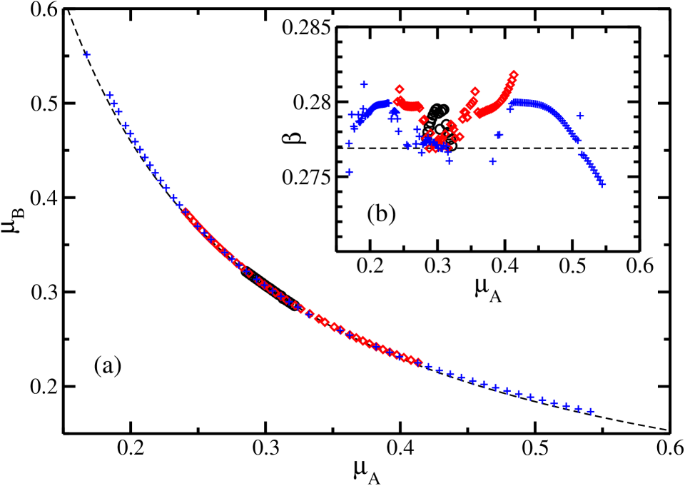
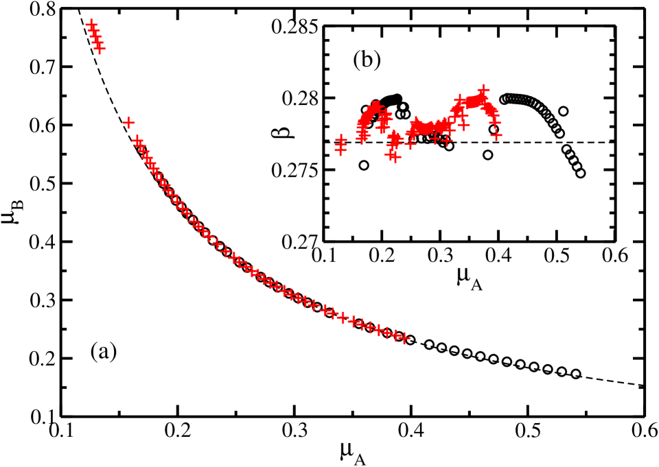
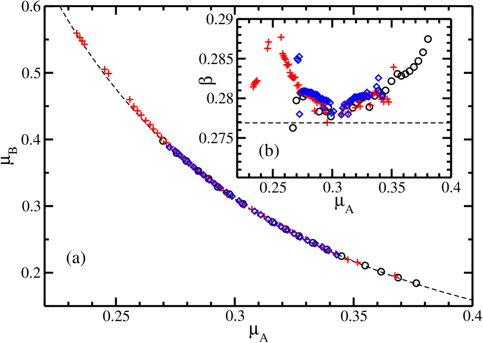
The series expansion for all three systems has been calculated up to order $N=24$. In order to evaluate how the estimates provided by the analysis described in Sec. III.2 behave with the order of the expansion, in Figs. 1 (a) and (b) the critical line and the critical exponent for the $AB$-lattice are shown for four different values of $N$, $N=\{10,17,24\}$. The points in Figs. 1 (a) and (b) were obtained after using transformation T1. Most notably, as seen in Fig. 1, the range of reliable critical points increases with increasing order $N$. Of course, the accuracy of the prediction also increases with increasing $N$. However, in general it can be said that even for low orders of the expansion the critical values are of good accuracy.

The critical exponents are more sensitive to the order of expansion – their behavior with $N$ is shown in the Fig. 1 (b). Not surprisingly, we find that with increasing order the critical exponents come closer to the best known value for the homogeneous CP from series expansions, $\beta\simeq 0.2769$ Jensen and Dickman (1993) – at least close to the homogeneous critical point. Further away from this point, all the critical exponents for all orders fluctuate between $\beta=0.275$ and $\beta=0.28$, the range in $\mu_{A}$ of reliable exponents coinciding with the range for the critical points.

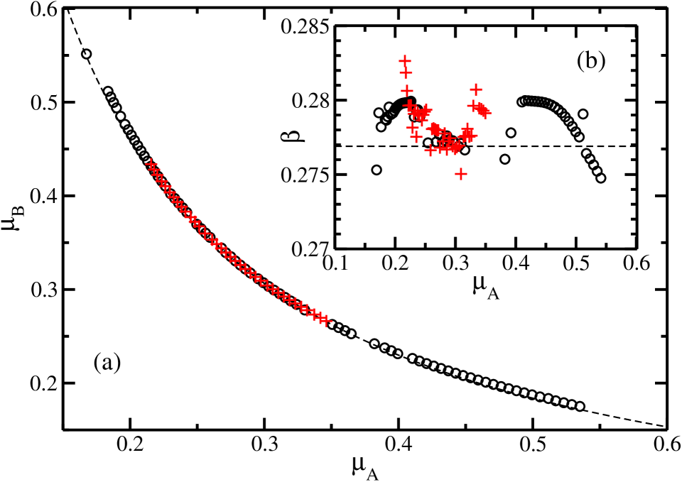
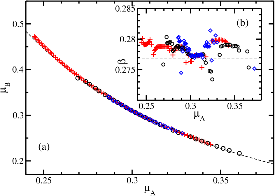
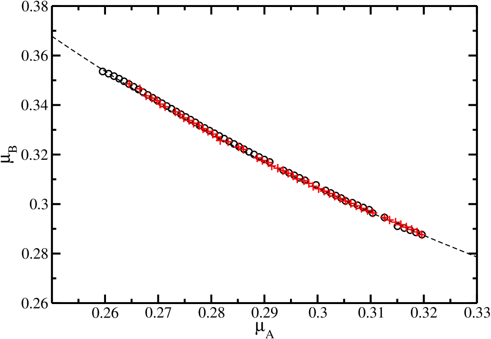
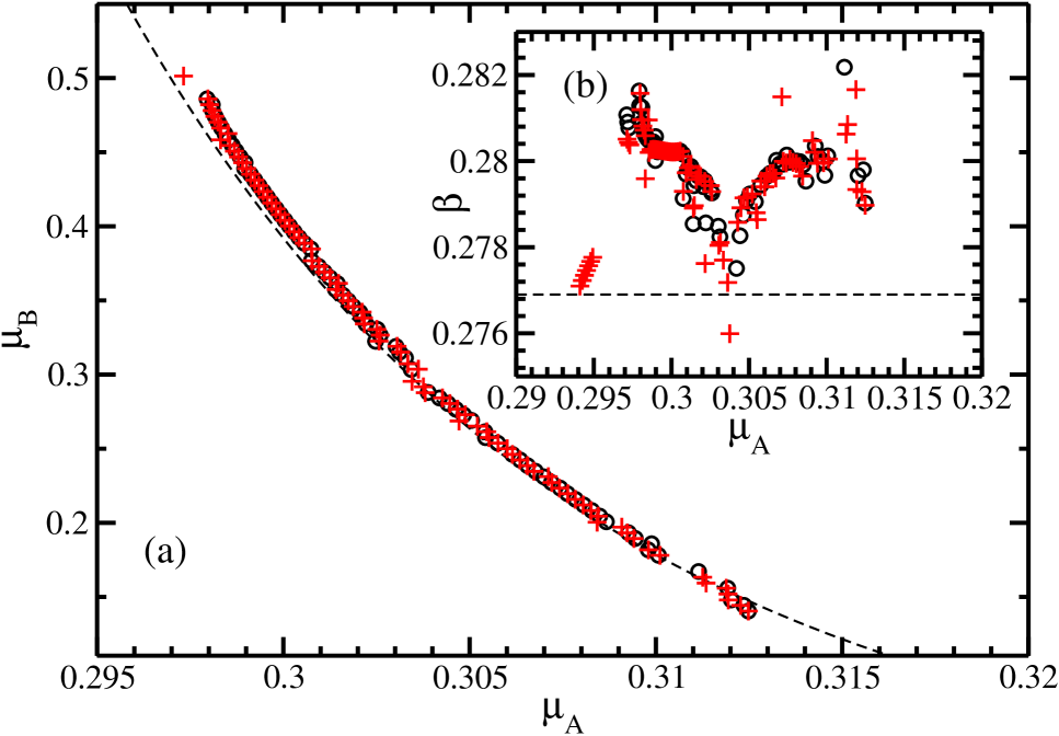
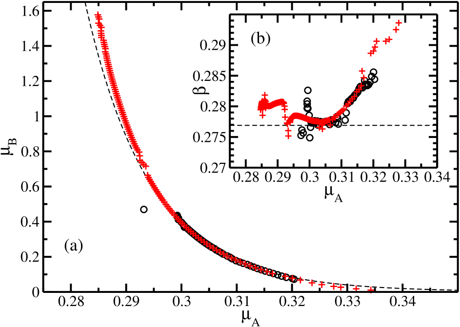
In an attempt to extend the range of applicability of the series expansion to locate critical points, the linear transformations described in Sec. III.2 are applied to the expansion variables. These transformations change the magnitude of the new variables $\bar{\mu}$ and $\delta$ and are therefore expected to provide extensions in different regions of the phase diagram. First, the transformations T1 and T2 are in employed in the $AB$ system (T3 being related by symmetry to T2). Fig. 2 shows that for this particular lattice the transformation T1 performs far better than T2 in giving stable critical points and critical exponents. The results of the transformations for the asymmetric system $AAB$ are compared in Figs. 3 (a) and (b). Here, two things are to note: transformation T2 extends the critical line further in the $\mu_{A}<\mu_{\text{c}}$ direction than T1 and T3 does in general poorly compared to the other two.

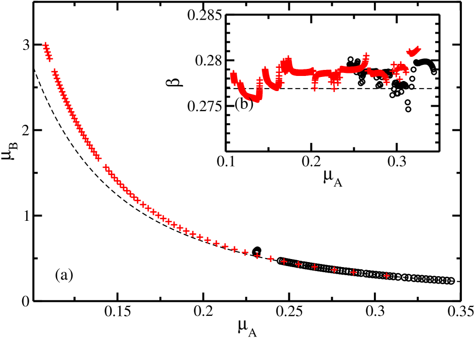
We also investigate the effects of different orders of Padé approximants for $\bar{\mu}$ and $\delta$ in the analysis as described in Sec. III.2. In order to do this, the steps given by Eqs. (21) and (22) are followed, but then, instead of taking the Padé approximant $\left[\mbox{$\lfloor(N-1)/2\rfloor$},\mbox{$\lceil(N-1)/2\rceil$}\right]_{\bar{\mu}}$ as shown in Eq. (23), the series in Eq. (22) is truncated at order $M<N-1$ in $\bar{\mu}$. This means that the coefficients of the terms $\bar{\mu}^{n}$ with $n\leq M$ that remain in the series are Padé approximants in $\delta$ formed from polynomials of degree larger than $N-1-M$. Therefore, the extrapolation provided by the Padé approximants of these coefficients can be expected to be more accurate than for polynomials of lower degree, which is the case for the coefficients of $\bar{\mu}^{n}$ for $n>M$. Then, the Padé approximant $\left[\mbox{$\lfloor M/2\rfloor$},\mbox{$\lceil M/2\rceil$}\right]_{\bar{\mu}}$ is taken. The results of such a cut-off is that the range of the convergence of the series is improved allowing for well behaved poles further away from the homogeneous critical point. The extension of the range for the phase-separation line achieved by this procedure can be seen in Figs. 4 (a) and 4 (b) for the $AAB$-system. For this system, the transformation T2 significantly extends the line of critical points into the region $\mu_{A}^{(\text{c})}<\mu_{\text{c}}$ and $\mu_{B}^{(\text{c})}>\mu_{\text{c}}$. In Fig. 4 (b), it can be seen that the critical exponents deviate from the value $\beta=0.2769$ by less than $1.2\%$.

The fact that this procedure of truncating in orders of expansion in $\bar{\mu}$ performs well in this particular case can be understood in the following manner. For the transformation T2, $\bar{\mu}=\mu_{A}$ and $\delta=\mu_{B}-\bar{\mu}=\mu_{B}-\mu_{A}$, leading to small values of the variable ($\bar{\mu}$) in which the expansion is cut, while $\delta$ is very large for $\mu_{A}<\mu_{\text{c}}$ and $\mu_{B}>\mu_{\text{c}}$. Therefore, we can expect the effects of dropping terms in $\bar{\mu}$ to be small while the benefit of only using Padé approximants in $\delta$ formed from high-order polynomials to be large. This explains the sizeable extension of the region in which the poles of the series are well-behaved.

In contrast to the $AAB$ system, the procedure described above does not produce much extension of the critical line for the $AB$ lattice, as can be seen Fig. 5: there are only a few points obtained by using transformation T2 further away from the homogeneous point than the critical points by the regular analysis with T1.

It is worth noting that the deviation of critical line from the line given by Eq. (32) appreciably increases away from the homogeneous critical point (see Fig. 4). It shows that Eq. (32) is only a lowest-order approximation in relation to the homogeneous critical point.

For the $AABB$ system, it is found that, in general, there is a smaller range of the critical values and critical exponents compared to the situation for $AB$ and $AAB$ chains. In order to investigate this difference in range of stability of the critical points and exponents, the $AABB$ critical line is compared with that for the $AB$ lattice, which should follow the same curve according to Eq. (32). It is found that the difference of the stability of the critical values seems to be a result of the number of unit cells that the series expansion takes into account. For order $N=24$, six unit cells on either side of the origin affect the series expansion for $AABB$ while the number is twice that for $AB$. If order $N=12$ expansion for the $AB$-lattice, which also only takes six unit cells into account, is compared with the order $N=24$ expansion for the $AABB$ chain, then we find that their ranges are very similar. This is shown in Fig. 6 where the critical points start to fluctuate wildly for both system at the same point in the phase diagrams (not presented in Fig. 6).

IV.1.2 Results obtained by PDA’s

As described in Sec. III.3, by applying the PDA method to the $P_{\infty}(\mu_{A},\mu_{A})$ we can also compute a line of critical points. The results obtained by this method depend on the choices of the label sets, $\mathbf{L}$, $\mathbf{M}$, $\mathbf{N}$ for the polynomials $P_{\mathbf{L}}(x,y)$, $Q_{\mathbf{M}}(x,y)$ and $R_{\mathbf{N}}(x,y)$ and the matching set $\mathbf{K}$. For all our analyses employing PDA’s, we use either label sets $\mathbf{M}$, $\mathbf{N}$ and $\mathbf{K}$ that have triangular or rectangular form. The label set $\mathbf{L}$ is then chosen to mimic the form of the others while at the same time making sure that the number of elements in all four sets satisfies the constraint that is imposed on them (see Sec. III.3). By ”triangular” label set $\mathbf{M}$ we mean that $(i,j)\in\mathbf{M}$ if $0\leq(i+j)\leq M_{max}$ while ”rectangular” refers to a set $\mathbf{M}$ for which $(i,j)\in\mathbf{M}$ if $0\leq i\leq M_{max,i}$ and $0\leq j\leq M_{max,j}$ with some integers $M_{max}$, $M_{max,i}$ and $M_{max,j}$. From here on, we will refer to a particular choice of the label sets $\mathbf{L}$, $\mathbf{M}$, $\mathbf{N}$ and matching set $\mathbf{K}$ as an input set.

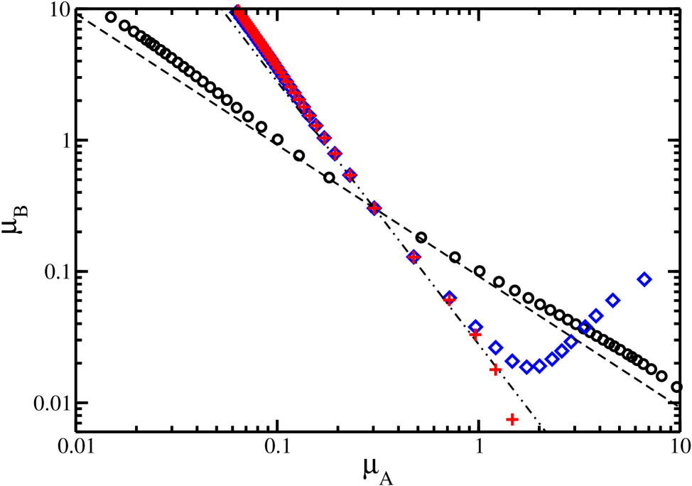
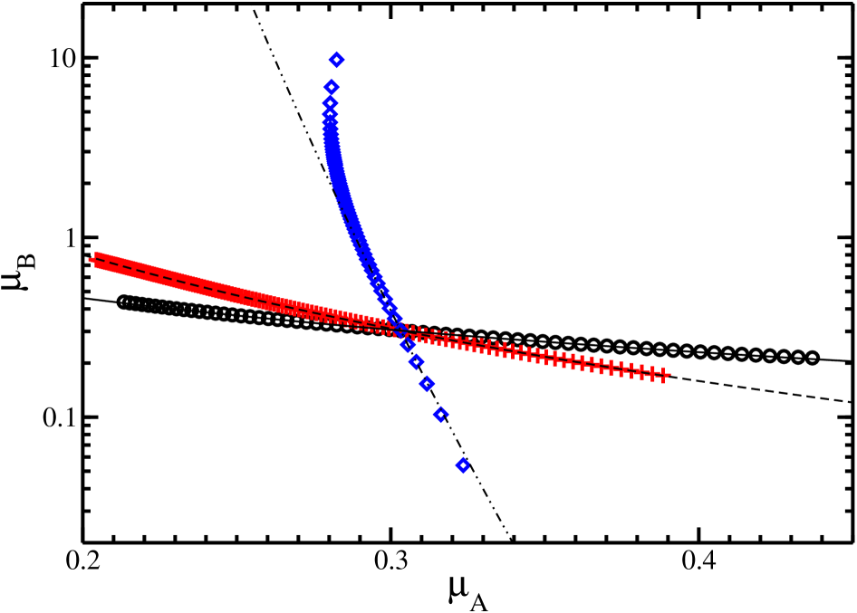
Often, different input sets produce critical lines of varying extent in $(\mu_{A},\mu_{B})$-space. In Fig. 7, we show the results from one input set for the $AB$ lattice and from two input sets for the $AAB$ lattice in comparison to the lines given by Eq. (32). The input set for the $AB$ lattice are triangular while the ones for the $AAB$ system are rectangular and triangular. The critical lines obtained by PDA’s are presented in $\log$-$\log$ scale because they extend to a rather wider range than those calculated by NPA’s (cf. Figs. 1, 3 and 7). One can clearly see that around the homogeneous critical point the lines from the series and described by Eq. (32) agree very well while deviations develop further away. It can be seen in Fig. 7 that the critical lines for triangular and rectangular input sets in the case of $AAB$ chain coincide in the vicinity of the critical point with a consistent tendency to be above the prediction given by Eq. (32). There is a point though where these two approximate curves for the critical line diverge: from there, the estimates given by the PDA’s can no longer be considered reliable (cf. the behavior of the curves marked by $+$ and $\diamond$ in Fig. 7 for $\mu_{A}\gtrsim 1$).

IV.2 Disordered Contact Process with Bimodal Distribution

IV.2.1 Results obtained by NPA’s

Figure 8: (Color online) Comparison of critical values (a) and critical exponents (b) of the disordered system with $p=0.5$ obtained from series expansions up to order $N=12$ using transformations T1 ($\circ$) and T2 ($+$). The dashed lines (     ) denote (a) the curve given by Eq. (32) and (b) the value for the critical exponent at the homogeneous critical point for the CP from series expansion, $\beta=0.2769$ Jensen and Dickman (1993).

Figure 9: (Color online) Comparison of critical values (a) and critical exponents (b) of the disordered system with $p=0.7$ obtained from series expansions up to order $N=12$: T1 ($\circ$), T2 ($+$) and T3 ($\Diamond$). The dashed lines (     ) denote (a) the curve given by Eq. (32) and (b) the value for the critical exponent at the homogeneous critical point for the CP from series expansion, $\beta=0.2769$ Jensen and Dickman (1993).

Figure 10: (Color online) Comparison of critical values (a) and critical exponents (b) of the disordered $1d$ lattice with $p=0.96$ obtained from series expansions up to order $N=12$ using exact configurational averaging ($\circ$) and approximate configurational averaging ($+$) with $k_{\text{max}}(12,p)=2$. In both expansions T1 was used. The dashed lines (     ) are given by Eq. (32) in (a) and by $\beta$ at the homogeneous critical point, $\beta=0.2769$, from series expansions Jensen and Dickman (1993) for the CP, in (b).

Figure 11: (Color online) Comparison of critical values (a) and critical exponents (b) of the disordered $1d$ lattice with $p=0.96$ obtained from series expansions of the approximately configurationally averaged survival probability up to order $N=19$ using the transformations T1 ($\circ$) and T2 ($+$). The dashed lines (     ) denote (a) the curve given by Eq. (32) and (b) the value for the critical exponent at the homogeneous critical point for the CP from series expansion, $\beta=0.2769$ Jensen and Dickman (1993).

Figure 12: (Color online) Critical lines in $\log$-linear scale for the disordered lattice with $p=0.5$ ($\circ$), $p=0.7$ ($+$) and $p=0.96$ ($\diamond$) as obtained by PDA’s: The three lines ( ), (     ) and ($\cdot\cdot$   $\cdot\cdot$) are given by Eq. (32) for the three disordered systems characterized by the values $p=0.5$, $p=0.7$ and $p=0.96$, respectively.

For the disordered CP, in which the recovery rates are drawn from the bimodal distribution given by Eq. (28), the same analysis as for the periodic lattices is carried out, with the only difference that the survival probability is configurationally averaged. Up to order $N=12$, the expansion of the survival probability can be configurationally averaged exactly for any value of $p$. The results for such systems characterized by $p=0.5$ and $p=0.7$ are shown in Figs. 8 and 9. For both values of $p$, the line of critical points and the critical exponents for the the two different linear transformations, T1 and T2, are compared.

Similar to the heterogeneous $AB$ lattice, we find that for the disordered system with $p=0.5$, transformation T1 extends the line of critical points furthest (see Fig. 8). The critical points are again well described by Eq. (32). The critical exponents, however, behave differently for the disordered case than for the heterogeneous lattices: while in the latter case they fluctuate up immediately away from homogeneous point $\mu_{\text{c}}$ but then fluctuate down again, in the former system, they almost linearly increase away from the homogeneous critical point.

Fig. 9 shows the results for the disordered lattice with $p=0.7$. This system behaves more like the heterogeneous $AAB$ lattice with transformation T2 extending the critical line furthest to the left, for $\mu_{A}<\mu_{\text{c}}$ and T1 furthest to the right, $\mu_{A}>\mu_{\text{c}}$. As usual, the points obtained from T3 lie in the middle and thus do not extend the critical line in any direction. The critical exponent $\beta$ displays very similar behavior as for $p=0.5$, mostly monotonically increasing away from the homogeneous critical point.

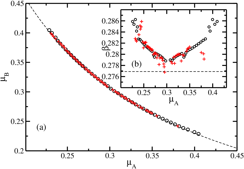
As noted in Sec. III.4, the exact configurational averaging of the survival probability, $\langle\mbox{$P_{\infty}$}\rangle$, becomes rapidly computationally very demanding with order of expansion and is only possible for $N\leq 12$. Therefore, the approximate scheme for averaging has to be applied for orders $N>12$. Such a scheme has been described in Sec. III.4. In order to test the reliability of this scheme, we analyze the disordered systems characterized by $p=0.96$, for which both exact and approximate averaging, with $k_{\text{max}}(12,p)=2$, are possible. The comparison between the two configurational averages are shown in Fig. 10 (a) and (b). It can be seen that the critical points agree very well for the two configurational averages where they both produce stable critical points, showing that the approximation scheme is indeed faithful for small disorder concentrations.

For a system with small concentration of $B$ sites, e.g. for $p\geq 0.96$, the approximate scheme described in Sec. III.4 can be applied for configurational averaging up to order $N=19$. Below, we present results for $p=0.96$ with $k_{\text{max}}(19,p)=2$. Figs. 11 (a) and (b) show the critical values and critical exponents for this case. Clearly, the transformation T2 works best for this system as is to be expected from its performance for the heterogeneous periodic $AAB$ lattice. The critical points from transformation T3 cover less range than T1 or T2, so we left these points out of Fig. 11. Deviation of the critical line from the curve given by Eq. (32) can be seen for $\mu_{A}<\mu_{\text{c}}$. The critical exponent $\beta$ increases monotonically with increasing value of $\mu_{A}$ away from the homogeneous critical point, $\mu_{A}>\mu_{\text{c}}$, while for $\mu_{A}<\mu_{\text{c}}$, significant fluctuations can be seen.

It should be mentioned that the critical line is only marginally extended by the procedure of cutting the series in different orders for $\bar{\mu}$ and $\delta$ described in the previous section.

IV.2.2 Results obtained PDA’s

Using similar input sets as for the heterogeneous systems (as described in Sec. IV.1.2), we apply PDA’s to the disordered systems as well. Generally, smaller input sets, with fewer elements in the label sets, are used because the series are shorter for the disordered systems but the triangular and rectangular shapes are still maintained. In Fig. 12, phase separation lines for three systems with the different degree of disorder characterized by the following values of $p=0.5$, $p=0.3$ and $p=0.96$ are shown. It can be clearly seen that Eq. (32) describes the critical lines obtained by the PDA’s very well around the homogeneous point. For the $p=0.96$ system, from $\mu_{B}=1.5$ the critical points deviate from Eq. (32). Consistent with the results from the NPA’s, the critical points obtained by PDA’s deviate above the line given by Eq. (32).

V Discussion & Conclusion

To conclude, we have presented a detailed description of the supercritical series expansions for the survival probability of the contact process in heterogeneous and disordered one-dimensional binary lattices. The heterogeneous systems are modeled by lattices with repeating patterns of sites of two types $A$ and $B$ characterized by different recovery rates, $\mu_{A}$ and $\mu_{B}$, and the disordered systems are represented by lattices of similar sites randomly placed on the lattice sites with probabilities $p$ and $1-p$, for nodes $A$ and $B$, respectively. For the analysis of the two-variable series (in $\mu_{A}$ and $\mu_{B}$), we have presented a scheme based on NPA’s in order to extract critical values and the critical exponent $\beta$ and have also used PDA’s to obtain estimates for the line of critical points.

It has been demonstrated that (i) using symmetric and asymmetric linear transformations, it is possible to extend the range of stable critical points in different regions of the rate-space $(\mu_{A},\mu_{B})$; (ii) keeping different orders in the Padé approximants with respect to the two variables, an extension of the line of critical points and an extended range for the critical exponents can be achieved; (iii) results from NPA’s and PDA’s compare well, PDA’s usually widening the range of the critical lines a bit further in the $(\mu_{A},\mu_{B})$-plane; (iv) an approximate scheme for configurational averaging can be applied in disordered lattices.

In general, the critical values can be reliably obtained by supercritical series expansions and they are in good agreement with the analytical approximation given by Eq. (32). For the critical exponents, the results are less conclusive due to larger errors, but certainly give some indication as to what happens to the universal critical behavior when spatial heterogeneity and disorder is introduced. For all heterogeneous lattices, we see fluctuations away from the best known value for the CP from series expansions, $\beta=0.2769$ Jensen and Dickman (1993), but they hardly ever exceed $\beta=0.28$ over the range of reliable points. This suggests that the CP for heterogeneous lattices still belongs to the DP universality class.

For the disordered systems, we see a qualitatively different picture. In general, we find that the critical exponents monotonically increase away from the value at the homogeneous critical point. As we were only able to compute the exact configurationally averaged survival probability up to order $N=12$ and an approximate one up to order $N=19$, we do not have very high precision, but the above tendency is clearly visible in all the data. This picture of continuously changing exponents is consistent with what a number of other authors Moreira and Dickman (1996); Cafiero et al. (1998); Dickman and Moreira (1998); Hooyberghs et al. (2003, 2004) have found and with the Harris criterion Harris (1974a).

VI Acknowledgments

The authors would like to thank I. Jensen, J. Stilck and S. V. Fallert for their helpful correspondence and remarks. The computations were partly performed on the Cambridge-Cranfield High-Performance Computer facility (HPCF) and the Cambridge University Condor Project. CJN would like to thank the UK EPSRC and the Cambridge European Trust for financial support.

Appendix A Selected series coefficients

Table 1: Series for the ultimate survival probability, $P_{\infty}=1-\sum_{n=1}^{N}\sum_{m=0}^{n}c_{nm}\mu_{A}^{n-m}\mu_{B}^{m}$, for the heterogeneous lattice $AB$ starting from a single occupied $A$-site up to order $N=15$ (continued in Tab. 2).

$n$	$m$	$c_{nm}$	$n$	$m$	$c_{nm}$	$n$	$m$	$c_{nm}$
0	0	1.00000000000000000000e+00		7	1.65000000000000000000e+01		12	-0.00000000000000000000e+00
				8	-0.00000000000000000000e+00
1	0	-1.00000000000000000000e+00				13	0	-1.00000000000000000000e+00
	1	-0.00000000000000000000e+00	9	0	-1.00000000000000000000e+00		1	-2.07000000000000000000e+02
				1	-6.80000000000000000000e+01		2	-6.74625000000000000000e+03
2	0	1.00000000000000000000e+00		2	-7.58500000000000000000e+02		3	-7.44351406860351562500e+04
	1	-2.00000000000000000000e+00		3	-1.69084472656250000000e+03		4	-3.01900451407580578234e+05
	2	-0.00000000000000000000e+00		4	3.02032038031683987356e+03		5	-2.76109780525427486282e+05
				5	1.11290729437934101043e+03		6	8.00284240250960225239e+05
3	0	-1.00000000000000000000e+00		6	-1.77129394531249909051e+03		7	4.74728979742886382155e+05
	1	5.00000000000000000000e-01		7	-4.27500000000000000000e+02		8	-3.91561916647056990769e+05
	2	-1.50000000000000000000e+00		8	-2.10000000000000000000e+01		9	-2.26055896148412110051e+05
	3	-0.00000000000000000000e+00		9	-0.00000000000000000000e+00		10	-3.99103976440429469221e+04
							11	-2.51875000000000000000e+03
4	0	1.00000000000000000000e+00	10	0	1.00000000000000000000e+00		12	-4.40000000000000000000e+01
	1	3.00000000000000000000e+00		1	9.40000000000000000000e+01		13	-0.00000000000000000000e+00
	2	-1.20000000000000000000e+01		2	1.45700000000000000000e+03
	3	3.50000000000000000000e+00		3	6.01312646484374818101e+03	14	0	1.00000000000000000000e+00
	4	1.02500000000000000000e+01		4	-7.55620689863017105381e+01		1	2.58000000000000000000e+02
				5	-1.94405384114583393966e+04		2	1.02715000000000000000e+04
5	0	-1.00000000000000000000e+00		6	4.71605225664304089150e+03		3	1.41998072448730497854e+05
	1	-9.00000000000000000000e+00		7	4.74978173828125090949e+03		4	7.83967321483503794298e+05
	2	1.02500000000000000000e+01		8	7.19500000000000000000e+02		5	1.54877796274059498683e+06
	3	-5.25000000000000000000e+00		9	2.60000000000000000000e+01		6	-8.33349567427633097395e+05
	4	-6.00000000000000000000e+00		10	-0.00000000000000000000e+00		7	-4.23806772828293405473e+06
	5	-0.00000000000000000000e+00					8	3.58496589470378821716e+05
			11	0	-1.00000000000000000000e+00		9	1.49872407836358295754e+06
6	0	1.00000000000000000000e+00		1	-1.25500000000000000000e+02		10	5.21977267719965777360e+05
	1	1.80000000000000000000e+01		2	-2.57100000000000000000e+03		11	7.00816817626952833962e+04
	2	2.44999999999999893419e+01		3	-1.59531196289062500000e+04		12	3.56925000000000000000e+03
	3	-1.21875000000000000000e+02		4	-2.17014048374422091001e+04		13	5.10000000000000000000e+01
	4	4.07500000000000000000e+01		5	4.88961204626596372691e+04		14	-0.00000000000000000000e+00
	5	9.00000000000000000000e+00		6	2.47395297945582315151e+04
	6	-0.00000000000000000000e+00		7	-2.65267486447097398923e+04	15	0	-1.00000000000000000000e+00
				8	-1.06594931640625000000e+04		1	-3.16500000000000000000e+02
7	0	-1.00000000000000000000e+00		9	-1.14000000000000000000e+03		2	-1.51542500000000000000e+04
	1	-3.05000000000000000000e+01		10	-3.15000000000000000000e+01		3	-2.55901594619751005666e+05
	2	-5.25000000000000000000e+00		11	-0.00000000000000000000e+00		4	-1.81766897669971594587e+06
	3	1.83769531250000000000e+02					5	-5.47577552606320381165e+06
	4	2.11445312500000213163e+01	12	0	1.00000000000000000000e+00		6	-3.39287989124816888943e+06
	5	-1.11250000000000000000e+02		1	1.63000000000000000000e+02		7	1.32761055815006103367e+07
	6	-1.25000000000000000000e+01		2	4.26500000000000000000e+03		8	8.67954126374729350209e+06
	7	-0.00000000000000000000e+00		3	3.62502430419921875000e+04		9	-5.72495353703939169645e+06
				4	9.72816786722543474752e+04		10	-4.44897483104257006198e+06
8	0	1.00000000000000000000e+00		5	-2.92123691227543495188e+04		11	-1.10378333697890699841e+06
	1	4.70000000000000000000e+01		6	-2.79344760523458826356e+05		12	-1.17472772171020405949e+05
	2	3.47500000000000000000e+02		7	4.62104999846149221412e+04		13	-4.93375000000000000000e+03
	3	1.52800781250000198952e+02		8	8.62397669988747074967e+04		14	-5.85000000000000000000e+01
	4	-1.45959277343750000000e+03		9	2.14371234130859302240e+04		15	-0.00000000000000000000e+00
	5	4.47820312500000113687e+02		10	1.72550000000000000000e+03
	6	2.33250000000000000000e+02		11	3.75000000000000000000e+01			continued in Tab. 2

Table 2: Series for the ultimate survival probability, $P_{\infty}=\sum_{n=16}^{N}\sum_{m=0}^{n}c_{nm}\mu_{A}^{n-m}\mu_{B}^{m}$, for the heterogeneous lattice $AB$ starting from a single occupied $A$-site up to order $N=24$ (continued from Tab. 1).

$n$	$m$	$c_{nm}$	$n$	$m$	$c_{nm}$	$n$	$m$	$c_{nm}$
16	0	1.00000000000000000000e+00		9	3.80933065114315605164e+09		9	9.19978211394436798096e+10
	1	3.83000000000000000000e+02		10	2.79066540292775917053e+09		10	-1.41663236622908508301e+11
	2	2.17725000000000000000e+04		11	-1.18839624965687608719e+09		11	-3.09544181677179382324e+11
	3	4.40507505485534784384e+05		12	-1.54566718886240291595e+09		12	-5.92025291294928512573e+10
	4	3.88379059831085987389e+06		13	-6.04278256410952091217e+08		13	1.17816956489996398926e+11
	5	1.58357353872441500425e+07		14	-1.20264935356224894524e+08		14	9.15751721367468566895e+10
	6	2.44039435816917717457e+07		15	-1.27080503243713695556e+07		15	3.26331674054245605469e+10
	7	-1.85767939421518109739e+07		16	-6.68376087843894492835e+05		16	6.70219656522058677673e+09
	8	-6.69576071585644334555e+07		17	-1.49485000000000000000e+04		17	8.07064469443650722504e+08
	9	4.24265176388191117439e+05		18	-9.35000000000000000000e+01		18	5.49525110365272164345e+07
	10	2.54600385214862190187e+07		19	-0.00000000000000000000e+00		19	1.94577521464836411178e+06
	11	1.14637431981598399580e+07					20	2.97977500000000109139e+04
	12	2.18359439378216117620e+06	20	0	1.00000000000000000000e+00		21	1.25000000000000000000e+02
	13	1.89539660865783487679e+05		1	7.39000000000000000000e+02		22	-0.00000000000000000000e+00
	14	6.67674999999999818101e+03		2	7.58940000000000000000e+04
	15	6.65000000000000000000e+01		3	2.78482589066410297528e+06	23	0	-1.00000000000000000000e+00
	16	-0.00000000000000000000e+00		4	4.77064398069097101688e+07		1	-1.11450000000000000000e+03
				5	4.30921612129856288433e+08		2	-1.66033750000000000000e+05
17	0	-1.00000000000000000000e+00		6	2.15946993785786914825e+09		3	-8.73441611697400361300e+06
	1	-4.58000000000000000000e+02		7	5.80407028293784332275e+09		4	-2.18288062553152590990e+08
	2	-3.05770000000000000000e+04		8	5.94638918469835090637e+09		5	-2.99289542933531618118e+09
	3	-7.29997349998474353924e+05		9	-7.40305007272274589539e+09		6	-2.41184413851611099243e+10
	4	-7.78990695947526767850e+06		10	-1.82033732679653511047e+10		7	-1.17519830906608703613e+11
	5	-4.04899793576145172119e+07		11	-2.40532317192275094986e+09		8	-3.41927873040872924805e+11
	6	-9.69540386525691747665e+07		12	7.10905857967732429504e+09		9	-5.02858276294200012207e+11
	7	-3.89085116880342364311e+07		13	4.71814863830389404297e+09		10	3.15742561692385902405e+10
	8	2.23379967691832602024e+08		14	1.42660811422320199013e+09		11	1.14735787437879589844e+12
	9	1.55998095356879800558e+08		15	2.35853332781435012817e+08		12	8.97016221831120605469e+11
	10	-8.29453441516727209091e+07		16	2.12726885021208114922e+07		13	-2.27905936943680297852e+11
	11	-8.40138382690373063087e+07		17	9.71620832698821439408e+05		14	-5.02435627291505371094e+11
	12	-2.68378383641524799168e+07		18	1.90230000000000000000e+04		15	-2.66655503063110687256e+11
	13	-4.09565602203018311411e+06		19	1.03500000000000000000e+02		16	-7.74699632413517761230e+10
	14	-2.96166594512939278502e+05		20	-0.00000000000000000000e+00		17	-1.35731640547505397797e+10
	15	-8.87100000000000000000e+03					18	-1.42167162412259006500e+09
	16	-7.50000000000000000000e+01	21	0	-1.00000000000000000000e+00		19	-8.53138949911509156227e+07
	17	-0.00000000000000000000e+00		1	-8.53000000000000000000e+02		20	-2.69011596571039920673e+06
				2	-9.97227500000000000000e+04		21	-3.67522500000000072760e+04
18	0	1.00000000000000000000e+00		3	-4.15225493661523098126e+06		22	-1.36500000000000000000e+02
	1	5.42000000000000000000e+02		4	-8.13538837860736250877e+07		23	-0.00000000000000000000e+00
	2	4.21000000000000000000e+04		5	-8.53730911617448449135e+08
	3	1.17137547012138389982e+06		6	-5.09422722262319755554e+09	24	0	1.00000000000000000000e+00
	4	1.48443261883842591196e+07		7	-1.72895074425995292664e+10		1	1.26300000000000000000e+03
	5	9.48619801399879902601e+07		8	-2.92424105203240814209e+10		2	2.10837500000000000000e+05
	6	3.07316159384340524673e+08		9	-2.19503462337732887268e+09		3	1.23666210482723508030e+07
	7	3.81732671278393089771e+08		10	6.57535642176373291016e+10		4	3.45435577848057389259e+08
	8	-3.78560457913966596127e+08		11	4.99555141215952529907e+10		5	5.34326366176584434509e+09
	9	-1.09090039428584504128e+09		12	-1.67071432757774791718e+10		6	4.91754102809474029541e+10
	10	-7.22351460704629123211e+07		13	-2.80141699739296989441e+10		7	2.78581107827627380371e+11
	11	4.26837997859395503998e+08		14	-1.29120452738848495483e+10		8	9.79218318459290283203e+11
	12	2.37199959095923602581e+08		15	-3.17061061754675102234e+09		9	1.98256718408773803711e+12
	13	5.84676568044034391642e+07		16	-4.44081987989710092545e+08		10	1.41222325451664990234e+12
	14	7.35058582342192064971e+06		17	-3.46190648118626475334e+07		11	-2.67964226093419287109e+12
	15	4.50249120122909313068e+05		18	-1.38645204595112707466e+06		12	-5.34463787449065527344e+12
	16	1.15980000000000000000e+04		19	-2.39322500000000000000e+04		13	-1.30437844961177197266e+12
	17	8.40000000000000000000e+01		20	-1.14000000000000000000e+02		14	1.94623313797743408203e+12
	18	-0.00000000000000000000e+00		21	-0.00000000000000000000e+00		15	1.74636441085664794922e+12
							16	7.14760408659765625000e+11
19	0	-1.00000000000000000000e+00	22	0	1.00000000000000000000e+00		17	1.74634440975768798828e+11
	1	-6.35500000000000000000e+02		1	9.78000000000000000000e+02		18	2.64786405199085998535e+10
	2	-5.69645000000000000000e+04		2	1.29406500000000000000e+05		19	2.43568212742165803909e+09
	3	-1.82815355796528002247e+06		3	6.07409790126359928399e+06		20	1.29837631260614901781e+08
	4	-2.71021273926327489316e+07		4	1.34919942776649802923e+08		21	3.66895718129834206775e+06
	5	-2.07776329672791510820e+08		5	1.62617631624924206734e+09		22	4.49402500000000072760e+04
	6	-8.53126758990889191628e+08		6	1.13523417998541107178e+10		23	1.48500000000000000000e+02
	7	-1.69019990104488110542e+09		7	4.67520642304774093628e+10		24	-0.00000000000000000000e+00
	8	-3.82997793883490979671e+08		8	1.07905537383186004639e+11

Table 3: Series for the configurationally-averaged ultimate survival probability, $\langle P_{\infty}\rangle=1-\sum_{n=1}^{N}\sum_{m=0}^{n}\langle c_{nm}\rangle\mu_{A}^{n-m}\mu_{B}^{m}$, for the disordered lattice with impurity concentration $p=0.5$ up to order $N=12$.

n	m	$\langle c_{nm}\rangle$	n	m	$\langle c_{nm}\rangle$	n	m	$\langle c_{nm}\rangle$
0	0	1.00000000000000000000e+00	7	0	-1.02856445312500000000e+00		4	8.57398099693330948412e+01
				1	6.71752929687499911182e+00		5	-1.59956149689860012586e+03
1	0	-5.00000000000000000000e-01		2	-7.88159179687500000000e+00		6	8.57398099692479576106e+01
	1	-5.00000000000000000000e-01		3	-3.63503417968750000000e+01		7	-3.78991681481602029180e+02
				4	-3.63503417968750000000e+01		8	3.15666996812323645827e+02
2	0	0.00000000000000000000e+00		5	-7.88159179687500000000e+00		9	-1.12182894054082581192e+02
	1	-1.00000000000000000000e+00		6	6.71752929687500000000e+00		10	1.97285068645925996123e+01
	2	0.00000000000000000000e+00		7	-1.02856445312500000000e+00
						11	0	-6.38827981592922071741e+01
3	0	1.25000000000000000000e-01	8	0	1.91795349121094105271e+00		1	2.76683537172620788169e+02
	1	-1.12500000000000000000e+00		1	-1.00450286865234925671e+01		2	-5.81148325010243183897e+02
	2	-1.12500000000000000000e+00		2	4.34407348632823939738e+01		3	1.08098985786890170857e+03
	3	1.25000000000000000000e-01		3	-1.05206558227552989138e+02		4	-1.09115308153965179372e+03
				4	-7.39358825683648177574e+01		5	-2.15854719928576787424e+03
4	0	2.18750000000000000000e-01		5	-1.05206558227541165706e+02		6	-2.15854719928370877824e+03
	1	-8.75000000000000000000e-01		6	4.34407348632839358515e+01		7	-1.09115308154012654995e+03
	2	2.18750000000000000000e-01		7	-1.00450286865224249766e+01		8	1.08098985786938828824e+03
	3	-8.75000000000000000000e-01		8	1.91795349121088110067e+00		9	-5.81148325010462372120e+02
	4	2.18750000000000000000e-01					10	2.76683537172492606260e+02
			9	0	-9.13367027706589240665e+00		11	-6.38827981592518412413e+01
5	0	1.56250000000000000000e-01		1	4.07988169988005395794e+01
	1	3.43750000000000000000e-01		2	-5.42188301086439778942e+01	12	0	1.82464000646571463449e+02
	2	-6.00000000000000000000e+00		3	6.09921527438696244872e+01		1	-9.07237726925243578080e+02
	3	-6.00000000000000000000e+00		4	-3.40893967946386396761e+02		2	2.01989525183668274622e+03
	4	3.43750000000000000000e-01		5	-3.40893967946387931534e+02		3	-2.51445338021211500745e+03
	5	1.56250000000000000000e-01		6	6.09921527438643025221e+01		4	4.03956355580561148599e+03
				7	-5.42188301086414981000e+01		5	-8.47482562600732853753e+03
6	0	3.45703125000000000000e-01		8	4.07988169988003761546e+01		6	-3.63662968564300990693e+03
	1	-1.91406250000000000000e-01		9	-9.13367027706600786985e+00		7	-8.47482562600957498944e+03
	2	-1.76757812500000000000e+00					8	4.03956355578774446258e+03
	3	-2.53984375000000000000e+01	10	0	1.97285068645884216210e+01		9	-2.51445338020943927404e+03
	4	-1.76757812500000000000e+00		1	-1.12182894054052439969e+02		10	2.01989525183534055941e+03
	5	1.56250000000000000000e-01		2	3.15666996812357751878e+02		11	-9.07237726928176357433e+02
	6	3.45703125000000000000e-01		3	-3.78991681481601744963e+02		12	1.82464000646704874953e+02

References

- Ódor (2004) G. Ódor, Rev. Mod. Phys. 76, 663 (2004).
- Hinrichsen (2000) H. Hinrichsen, Advances in Physics 49, 815 (2000).
- Janssen (1981) H. K. Janssen, Z. Phys. B 42, 151 (1981).
- Grassberger (1982) P. Grassberger, Z. Phys. B 47, 365 (1982).
- Harris (1974a) A. B. Harris, J. Phys. C 7, 1671 (1974a).
- Liggett (1985) T. Liggett, Interacting Particle Systems (1985), 1st ed.
- Moreira and Dickman (1996) A. G. Moreira and R. Dickman, Phys. Rev. E 54, R3090 (1996).
- Cafiero et al. (1998) R. Cafiero, A. Gabrielli, and M. A. Muñoz, Phys. Rev. E 57, 5060 (1998).
- Dickman and Moreira (1998) R. Dickman and A. G. Moreira, Phys. Rev. E 57, 1263 (1998).
- Hooyberghs et al. (2003) J. Hooyberghs, F. Iglói, and C. Vanderzande, Phys. Rev. Lett. 90, 100601 (2003).
- Hooyberghs et al. (2004) J. Hooyberghs, F. Iglói, and C. Vanderzande, Phys. Rev. E 69, 66140 (2004).
- Vojta and Dickison (2005) T. Vojta and M. Dickison, Phys. Rev. E 72, 36126 (2005).
- Dickman and Jensen (1991) R. Dickman and I. Jensen, Phys. Rev. Lett. 67, 2391 (1991).
- Jensen and Dickman (1993) I. Jensen and R. Dickman, J. Stat. Phys. 71, 89 (1993).
- Guillaume (1997) P. Guillaume, J. Comp. Appl. Math. 82, 149 (1997).
- Guillaume and Huard (2000) P. Guillaume and A. Huard, J. Comp. Appl. Math. 121, 197 (2000).
- Dantas and Stilck (2005) W. G. Dantas and J. F. Stilck, J. Phys. A: Math. Gen. 38, 5841 (2005).
- Harris (1974b) T. Harris, Annals of Probability 2, 969 (1974b).
- Doi (1976) M. Doi, J. Phys. A 9, 1479 (1976).
- Peliti (1985) L. Peliti, J. Physique 46, 1469 (1985).
- Baker and Graves-Morris (1996) G. Baker, Jr. and P. Graves-Morris, Padé Approximants (Cambridge University Press, 1996), 2nd ed.
- Guttmann (1989) A. J. Guttmann, in Phase Transitions and Critical Phenomena Vol. 13, edited by C. Domb and J. L. Lebowitz (Academic Press, London, 1989).
- Bender and Orszag (1978) C. Bender and S. Orszag, Advanced Mathematical Methods for Scientists and Engineers (McGraw-Hill, 1978), 1st ed.
- Chisholm (1973) J. S. R. Chisholm, Mathematics of Computation 27, 841 (1973).
- Fisher and Kerr (1977) M. E. Fisher and R. M. Kerr, Phys. Rev. Lett. 39, 667 (1977).
- Fisher (1977) M. E. Fisher, Physica B 86-88, 590 (1977).
- Styer (1990) D. F. Styer, Comp. Phys. Comm. 61, 374 (1990).
- Stilck and Salinas (1981) J. F. Stilck and S. R. Salinas, J. Phys. A: Math. Gen. 14, 2027 (1981).
- Neugebauer et al. (2006) C. J. Neugebauer, S. V. Fallert, and S. N. Taraskin, Phys. Rev. E 74, 040101(R) (2006).